ISPRS Annals of the Photogrammetry, Remote Sensing and Spatial Information Sciences, Volume IV-2, 2018 ISPRS TC II Mid-term Symposium “Towards Photogrammetry 2020”, 4–7 June 2018, Riva del Garda, Italy
NEURAL NETWORKS FOR THE CLASSIFICATION OF BUILDING USE FROM STREET-VIEW IMAGERY Dominik Laupheimer 1, *, Patrick Tutzauer 1, Norbert Haala 1, Marc Spicker 2 1 Institute
for Photogrammetry, University of Stuttgart, Germany - (dominik.laupheimer, patrick.tutzauer, norbert.haala)@ifp.unistuttgart.de 2 Visual Computing Group, University of Konstanz, Germany -
[email protected] Commission II, WG II/6
KEY WORDS: Urban Data, Image Classification, Convolutional Neural Networks, Feature Learning, Class Activation Maps ABSTRACT: Within this paper we propose an end-to-end approach for classifying terrestrial images of building facades into five different utility classes (commercial, hybrid, residential, specialUse, underConstruction) by using Convolutional Neural Networks (CNNs). For our examples we use images provided by Google Street View. These images are automatically linked to a coarse city model, including the outlines of the buildings as well as their respective use classes. By these means an extensive dataset is available for training and evaluation of our Deep Learning pipeline. The paper describes the implemented end-to-end approach for classifying street-level images of building facades and discusses our experiments with various CNNs. In addition to the classification results, so-called Class Activation Maps (CAMs) are evaluated. These maps give further insights into decisive facade parts that are learned as features during the training process. Furthermore, they can be used for the generation of abstract presentations which facilitate the comprehension of semantic image content. The abstract representations are a result of the stippling method, an importance-based image rendering. 1. INTRODUCTION Data collection to generate and update 3D virtual city models has become a standard task in photogrammetry and computer vision. As an example, multi-view stereo image matching can automatically extract 3D urban models consisting of complex and dense surface triangle meshes, which allow for visually appealing representations. However, semantic information is additionally required to provide meaningful 3D building models for applications such as interactive navigation, urban planning, computational engineering and video games. 1.1 Related Work A general task to be solved in this context is to separate the urban scene into objects like buildings, streets or vegetation. For this purpose, Weinmann et al. (2015) apply classifiers like Support Vector Machines or Random Forests on 3D point clouds from mobile mapping. By these means they use the Oakland 3D Point Cloud Dataset to discriminate between the semantic labels wire, pole/trunk, facade, ground and vegetation. Another experiment separates the Paris-rue-Madame 3D point cloud database into the classes facade, ground, cars, motorcycles, traffic signs and pedestrian. Similarly, Verdie et.al. (2015) analyze geometric attributes by applying a Markov Random Field (MRF). Their experiments use surface meshes generated by multi-view stereo from airborne imagery to classify ground, tree, facade and roof. Recent approaches simultaneously reconstruct 3D urban scenes from imagery while reasoning about the semantic content, e.g. by projecting 2D image segmentations into the point cloud (Vineet et al., 2015). Cherabier et al. (2016) and Blaha et al. (2016) aim to solve the multi-labeling problem at large scales in a volumetric domain. This supports the 3D reconstruction by removing undesired objects or introducing class-specific shape priors. Within the 2D image domain, Badrinaralyanan et al. (2017) present SegNet, a new state-of-the-art CNN-based segmentation approach
for urban scenes with classes such as building, street, sidewalk, cars, and pedestrians. SegNet is based on a deep convolutional encoder-decoder structure. The decoder applies transferred pool indices from the encoder to generate a sparse features map. The algorithm subsequently uses a filter bank to densify those feature maps, concluding with a pixel-wise classification layer. Earlier works in the reviving era of Deep Learning investigate hierarchical feature learning using a multiscale CNN and report results on urban scenes in the SIFT Flow dataset (Farabet et al., 2013). There are several papers using SIFT/SURF and a clustering approach, trying to identify features that are characteristic for a certain city or visual cues that lead to different perceptions of city scenes (Doersch et al., 2012; Quercia et al., 2014). Recent work picks up this idea and trains a Siamese-like convolutional neural architecture on image pairs to predict perception of urban scenes (Dubey et al., 2016). Branson et al. (2018) adapt state-of-the-art CNN-based object detectors and classifiers to catalog trees from aerial and street-level imagery. The approach consists of two modules - generation of a geographic catalogue of objects for a given location and computation of fine-grained class labels for the 3D object at the given location. Yu et al. (2015) aim on large scale detection of business store fronts using Multibox, a single CNN architecture directly generating bounding box candidates and their confidence scores from image pixel input. Training data consists of two million manually labeled panoramas as provided by crowdsourcing. Workman et al. (2017) fuse aerial and street-level imagery to classify land use, building function and building age. Aforementioned work focuses on separating urban scenes into different object types. Extensive research is conducted in the more specific task of facade analyzation. Martinovic et al. (2015) propose a complete pipeline from SfM-based reconstruction to semantic labeling of street-side scenes. They perform classification of 3D point clouds as provided by a multi-view-stereo reconstruction into semantic classes window, wall, balcony, door, roof,
* Corresponding author
This contribution has been peer-reviewed. The double-blind peer-review was conducted on the basis of the full paper. https://doi.org/10.5194/isprs-annals-IV-2-177-2018 | © Authors 2018. CC BY 4.0 License.
177
ISPRS Annals of the Photogrammetry, Remote Sensing and Spatial Information Sciences, Volume IV-2, 2018 ISPRS TC II Mid-term Symposium “Towards Photogrammetry 2020”, 4–7 June 2018, Riva del Garda, Italy
sky and shop using a Random Forest classifier trained on lightweight 3D features. Gadde et al. (2016) segment 2D images and 3D point clouds of building facades and present empirical results on all available 2D and 3D facade benchmark datasets. Symmetries in the facade imagery can also be exploited by applying specific shape priors for energy minimization (Teboul et al., 2010; Wenzel and Förstner, 2016). Mathias et al. (2016) present a three layered approach consisting of an initial semantic segmentation, the subsequent object detection and a final layer introducing building-specific meta-knowledge by so-called weak architectural principles. 1.2 Classification of Street-Level Images by CNNs Our approach aims on the classification of building facades in street-view images into use classes commercial, hybrid, residential, specialUse, and underConstruction. For this purpose CNNs are used, which are a powerful tool for tasks like object recognition (Russakovsky et al., 2015). We leverage Google’s region wide available Street View data. The ground truth data consists of the digital city base map provided by the City Survey Office Stuttgart. Such coarse city models are frequently available from National Mapping and Cadastral Agencies. Our data consists of a 2D ground plan polygon for each building, enriched with semantic information like address, communal district, building block number and building use. We link this information to the respective street level images based on positions and headings as provided by the Street View API (Google Developers, 2017). The implemented framework aims on the differentiation of five rather general use classes. The classes commercial and residential are defined for a singular use of a building, while the class hybrid represents a mixture of these two use classes – e.g. shops and apartments in the same building. The class specialUse represents the remaining buildings not matching the other three classes, like schools and churches. Finally, the class underConstruction contains buildings being under construction, independent of their actual use. These classes are purely defined by the cadastral data and therefore are not constrained to a particular visual appearance of facades. Main contributions of our work are: (1) a CNN based approach to classify street-level facade imagery from (semi-) automatically generated training data. (2) We compare several pretrained versus non pretrained CNN architectures and show that pretrained models significantly improve accuracy, although the dataset for pretrained models (ImageNet) differs considerably from ours. (3) By using CAMs we get insights into important areas for the classification. (4) Moreover, we can localize problematical zones. Hence, the “blackbox dogma” of Deep Learning is softened. (5) As an application for our approach we show facade stipplings - importance-based image renderings that are steered by CAMs. These stippled images could facilitate the understanding of the semantic content of original images, like different building categories. The following section 2 presents the setup of our CNN framework. This includes steps like the selection of a suitable network architecture as well as the training of the network with suitable ground truth data. Section 3 presents the performance evaluation of our end-to-end approach on different datasets with various CNNs. Section 4 then further examines which features are learned during the training process. For this purpose we make use of CAMs, visualizing areas being important for the network’s decision. In addition to visualizing learned features by the classification process, we use CAMs to produce abstract renderings that simplify the visual content of our input images. As described in section 5, non-photorealistic rendering can guide the viewer’s attention by varying the level of abstraction (Gooch and Gooch, 2001). In our case we want to focus the user’s
attention to regions which are deemed important by the Class Activation Maps, thereby helping users to grasp the building’s category more easily. 2. SETUP AND TRAINING OF THE CNNS CNNs are mapping functions solving classification tasks by a huge amount of learnable parameters. These learnable parameters are arranged in convolutional kernels, which can be interpreted as feature detectors after being trained. CNNs do not require handcrafted features or feature detectors as parameters are adjusted without human interaction during the training process. Setting up a CNN requires the selection of suitable architectures defined by the amount of kernels and layers, the type of activation function as well as hyperparameters (i.e. non-learnable parameters). Figure 1 depicts the architecture of a CNN for multiclass classification with an input layer, multiple hidden layers and an output layer. The input layer is tailored to the specific application, in our case street-level RGB images of size 400x400x3 pixels (see section 2.1). The amount of considered classes defines the size of the output layer which represents the estimated label vector . The depth of hidden convolutional layers depends on the amount of used convolutional kernels applied to the previous layer. Each convolutional kernel creates a so-called activation map which is a depth slice of a hidden layer.
Figure 1. Architecture of a CNN for multiclass classification. Our investigations use state-of-the-art architectures like VGG16, VGG19 (Simonyan and Zisserman, 2014), ResNet50 (He et al., 2016) and InceptionV3 (Szegedy et al., 2016) which have already been applied successfully for several classification tasks. Furthermore, we design networks with less amount of layers and kernels (i.e. less amount of learnable parameters). In our experiments we focus on reducing the amount of parameters, and therefore the training time, while trying to conserve the overall accuracy compared to state-of-the-art networks. The best-performing self-designed network is a VGG-alike network that consists of 8 convolutional layers. One convolutional layer performs 1x1 convolutions in order to reduce the amount of trainable parameters. The layers of the network are: two convolutional layers (16 feature maps each), a max pooling layer with stride 2, two convolutional layers (64 feature maps each), a max pooling layer with stride 2, one 1x1 convolutional layer (16 feature maps), two convolutional layers (256 feature maps each), a max pooling layer with stride 2, one convolutional layer (1024 feature maps), a global max pooling layer, two fully connected layers with 1024 classes. All layers neurons each, and an output layer with (except the output layer) use the ReLU activation function. The output layer uses the softmax activation function. In total, the network consists of 8 convolutional layers, 1456 features and makes use of 4.16 million parameters (for 400x400x3 sized images and neglecting the reasoning part consisting of fully connected layers). In comparison to that, the VGG16 network consists of 13 convolutional layers, 4224 features and makes use of 14.71 million parameters (for 400x400x3 sized images and neglecting the reasoning part consisting of fully connected layers). This means our best-performing self-designed network uses only 28.24% of the amount of parameters a VGG16 network uses. VGG19, ResNet50 and InceptionV3 use even more parameters. We use Keras 2.04 (Chollet et al., 2015) for the implementation and train on a machine using a Titan X Pascal GPU (12GB). The
This contribution has been peer-reviewed. The double-blind peer-review was conducted on the basis of the full paper. https://doi.org/10.5194/isprs-annals-IV-2-177-2018 | © Authors 2018. CC BY 4.0 License.
178
ISPRS Annals of the Photogrammetry, Remote Sensing and Spatial Information Sciences, Volume IV-2, 2018 ISPRS TC II Mid-term Symposium “Towards Photogrammetry 2020”, 4–7 June 2018, Riva del Garda, Italy
following section 2.1 describes the preparation of suitable data for training, validation and testing. Section 2.2 depicts the training step. Classification results are discussed in section 3 afterwards.
of the fact that this lowers the performance (see Figure 7), but it is unavoidable in an only class-aware setting as street-level images almost always contain more than one building.
2.1 Preparation of Data One of the main burdens for training a CNN is the need for large amount of labeled data. As there is no benchmark for our purposes, we have to prepare labeled data on our own. For this reason we obtain street-level RGB images by crawling Google Street View imagery from Stuttgart and link it to 2D cadastral data provided by the City Survey Office Stuttgart (Tutzauer and Haala, 2017). The 2D cadastral data consists of polygons enriched with semantic information (amongst others the building use) for each building. By using positions and heading information of the crawled Google Street View images, this cadastral information is linked to the respective street level images. Cadastral data distinguishes between approximately 300 different building use types. Hence, the linking of information results in a fine-grained labeling, initially. Regarding class separability this comes in handy, but regarding training this is suboptimal as every class needs a large amount of training samples. Since creating a labeled dataset is a very tedious task, we gather the finegrained labels into our 5 coarse classes: commercial, hybrid, residential, specialUse and underConstruction. As an example, buildings with cadastral building use single-family house or multi-family house are sorted into our more general class residential. Mathematically, the labels are represented as label vectors of , where the class-corresponding entry is one and all size other entries are zero (one-hot vector). All images ( ) form the . set of images : = ( ) ∈ 1, … , Hence, labeled datasets for image classification consist of images ( ) labeled with correspondent one-hot ground truth label vectors ( ) (also known as target vectors). In other words, datasets consist of tuples ( ) , ( ) . We consider good training samples as frontal shots of facades that are not obstructed by vegetation, vehicles and such. Frontal shots are ensured by taking into account the heading information of the Google Street View images and the estimated normal vector of the facades’ front. We constrain viewing angles onto facades not being too large (with respect to facade normal vector). This constraint excludes all images with a viewing direction aligned with the street direction, thus, showing many facades. Avoiding obstructed imagery was achieved by employing a Fully Convolutional Network (FCN, Long et al., 2015) and analyzing image content by pixel-wise segmentation in previous work (Tutzauer and Haala, 2017). We process the pixel-wise FCN segmentation to ensure that facades are not too heavily occluded. Thus, samples with too many pixels depicting vegetation or vehicles are discarded. However, FCN inference is time-consuming and labels are only class-aware, not instance-aware. For our purpose it is desirable to distinguish between different object instances. Therefore, we trained an implementation of Faster R-CNN (Ren et. al, 2015; Henon, 2017) on a subset of the Open Images Dataset (Krasin et al., 2016) from scratch. We used three classes: building, tree (container class for vegetation) and automobile (container class for vehicles) with around 23.200, 45.500 and 34.200 images, respectively. Figure 2 shows some exemplary results. While the dataset at hand was generated with the aforementioned FCN processing, future work should rely on the described Faster R-CNN approach. To emphasize this point: our data at hand performs image classification. Each image is associated with a one-hot label vector. The human-given label corresponds to the building in the center of the image. We are aware
Figure 2. Examples of Faster R-CNN object detection on our extracted Street View imagery. Obviously, in the real world there are more facades of residential buildings than facades belonging to other classes causing an imbalanced dataset, initially. With the help of a priori data augmentation (horizontal flipping, warping, cropping, jittering and modification of saturation) we create an equally distributed dataset with the same amount of samples for every class. Our final training set is a balanced dataset consisting of 75.000 labeled images in total (15.000 images per class). Validation set and test set consist of 350 labeled images each (70 images per class). The comparatively small size of the test and validation set is due to the dataset split before data augmentation. Data augmentation is only applied to the training set in order to prevent overfitting. Augmenting validation set and test set would bias the achieved results in a positive way. In addition to this multiclass (5-class) dataset, we provide datasets with reduced amount of classes. The binary datasets residential vs. nonResidential and underConstruction vs. notUnderConstruction as well as a 3-class dataset with classes commercial, hybrid and residential are used to investigate the impact of class definitions to the classification performance. All provided datasets are split into three parts: images for training (training set), images for validating the network’s performance during the training process (validation set) and images for evaluating the network’s performance after the training process (test set). 2.2 Training In a nutshell, training of CNNs is an optimization task minimizing a cost function that measures the mean discrepancy between predicted label vectors ( ) and ground truth label vectors ( ) for all training images ( ) We use the discrete cross() () entropy , for each image ( ) (see Equation 1) as cost function (summation over classes , arbitrary base , amount of images ). =
1
()
,
()
=−
1
()
( ) log
()
( ) (1)
Parameters are initialized using Glorot uniform initialization (Glorot and Bengio, 2010), while updating is based on backpropagation (LeCun et al., 1998) in combination with Stochastic Gradient Descent. Generally, the cross-entropy decreases during
This contribution has been peer-reviewed. The double-blind peer-review was conducted on the basis of the full paper. https://doi.org/10.5194/isprs-annals-IV-2-177-2018 | © Authors 2018. CC BY 4.0 License.
179
ISPRS Annals of the Photogrammetry, Remote Sensing and Spatial Information Sciences, Volume IV-2, 2018 ISPRS TC II Mid-term Symposium “Towards Photogrammetry 2020”, 4–7 June 2018, Riva del Garda, Italy
training when evaluated on training data. Naturally, this comprises overfitting which means that the noise of training data is learned. To avoid overfitting, we use validation data during training to keep track on the generalization gap - the difference between performance on training data and validation data. Moreover, we use regularization methods like early stopping, weight decay and dropout (Srivastava et al., 2014) in order to reduce overfitting. During training, parameters are adjusted so that the desired task i.e. the classification of building facades in Google Street View images into the respective use classes is accomplished. After training, a network’s performance is analyzed by using images with known ground truth data that have not been used during training (see section 3). If performance on this test set is appealing, the trained network can be used as a black box for classifying any new unseen data into desired classes. 3. CLASSIFICATION RESULTS Amongst the investigated networks, an InceptionV3 network pretrained on ImageNet images performs best with an overall accuracy of 64.00% when being evaluated on our 5-class test set. Its colored normalized confusion matrix (NCM) is shown in Figure 3. The diagonal elements represent per-class accuracies (in case of NCM, these equal per-class recall values). Per-class precision values can be calculated by dividing the diagonal elements by corresponding column sums. The best performing class (residential) achieves an accuracy of 98.57%, which is pleasant as the majority of real-world buildings are residential buildings. On the other hand, classes specialUse and underConstruction only achieve accuracies of 25.71% and 48.57%, respectively. This is due to the classes’ definitions (see Section 1.2). Class specialUse has high intra-class variance and therefore bad separability from other classes. Class underConstruction “hovers” over all other classes. Frequently, an image of class underConstruction differs only from other classes by a scaffold. Normally, scaffolds are of small size in the image and hard to detect by a computer. In contrast, the per-class precision of those two classes is high (90.00% and 94.44% respectively).
Figure 3. Normalized confusion matrix of the bestperforming network (pretrained InceptionV3 on ImageNet) when being evaluated on our 5-class test set. Other current state-of-the-art models (VGG16, VGG19, ResNet50) perform slightly worse (see Table 1). For pretraining we used ImageNet images. We observed that pretraining improved the performance by 8-10% - although ImageNet images and images of our datasets differ significantly. Our best-performing self-designed network could achieve 52.29% overall accuracy while reducing the amount of parameters by approximately 72% (relative to VGG16, see section 2).
The self-designed network was purely trained on our 5-class training set. The achieved overall accuracy is slightly worse than the overall accuracies of not-pretrained VGG-networks (not-pretrained VGG16: 55.43%, not-pretrained VGG19: 53.43%). Training time per epoch reduces to 26.3 min/epoch (VGG16: 54.5 min/epoch, VGG19: 62.5 min/epoch). Table 1. Highest achieved overall accuracies of different CNNs on our balanced 5-class test set. All networks have been pretrained on ImageNet images. network VGG16 VGG19 ResNet50 InceptionV3
overall accuracy [%] 63.43 63.14 55.43 64.00
In addition to our performance analysis for five classes we further used 2-class and 3-class datasets to analyze effects of class separability and intra-class variance on the classification performance. Correspondingly, we train binary and 3-class classifiers. Results of our 2-class and 3-class classifiers prove that better class separability and reduced intra-class variance have a crucial impact on the achieved overall accuracy. The binary classifiers (residential vs. noResidential and underConstruction vs. notUnderConstruction) achieve an overall accuracy of approximately 88%. Our 3-class classifier achieves an overall accuracy of approximately 73%.
Figure 4. Correctly classified images with corresponding upsampled CAMs overlaid (binary classification). The respective color of the CAM represents the importance regarding the network’s prediction. 4. LOCALIZATION OF CLASS-SPECIFIC IMAGE REGIONS BY CAMS In addition to the classification results, CNNs can provide Class Activation Maps as additional output, which are a powerful tool to interpret and localize learned features within input images. CAMs are heatmaps that highlight image sections, which are discriminant for the respective classification process. Thereof, a
This contribution has been peer-reviewed. The double-blind peer-review was conducted on the basis of the full paper. https://doi.org/10.5194/isprs-annals-IV-2-177-2018 | © Authors 2018. CC BY 4.0 License.
180
ISPRS Annals of the Photogrammetry, Remote Sensing and Spatial Information Sciences, Volume IV-2, 2018 ISPRS TC II Mid-term Symposium “Towards Photogrammetry 2020”, 4–7 June 2018, Riva del Garda, Italy
human operator can derive learned features which are useful for understanding the networks decisions.
the CNN pipeline convolves and pools the original image several times, which reduces the original spatial dimension. Figure 4 shows correctly classified images for the binary classification overlaid by the associated upsampled CAMs which highlight decisive image parts. Please note the importance of the vegetation in the right image of the first row for a correct prediction. Figure 5 shows correctly classified images for the 5-class classification overlaid by the associated upsampled CAMs. The right image in the third row shows a kindergarten. Please note that the big windows with the window decorations attract the network’s attention. Images overlaid with CAMs give insight about the features learned for decision making. Similar to features a human operator would use instinctively, a CNN uses “facade-related” information like rooftops, windows and chimneys as well as contextual information like trees, cars and sky. CAMs give a hint on image areas that are crucial for image labeling. This can be used to analyze potential misclassifications. As it is visible from the depicted examples in Figure 6, misclassifications frequently result from features, which are not detected by the CNN or from features, which are misinterpreted. The restaurant with accommodation on the left side in the first row in Figure 6 is classified as specialUse due to its church-alike entrance. Besides, dormers are not detected. The church on the right side in the first row is classified as residential as the bell tower might be mistaken as a chimney. The lower left image shows a residential building with many windows and satellite dishes. As the satellite dishes are not detected, the building looks similar to an office building (commercial). The lower right image shows a residential image with traffic signs in the front. Certainly, they are mistaken as advertisement panels leading to prediction hybrid. As it is also visible (see Figure 7), the choice of ground truth label has an influence on the classification performance. From a human point of view the building in the image center is decisive for labeling. In contrast, CNNs simply decide by using those features with the most impact on predictions. The location and size within the image do not matter. Hence, predicted and ground truth labels can differ, although basically, both are correct. Such predictions still are lowering the overall accuracy if they do not match the human-given label. We refer to this type as “false” predictions as they are not necessarily false. Figure 7 shows such a “false” prediction where the residential building and the vegetation on the right hand side in the image cause the prediction residential. On the contrary, the transformer house in the image center is decisive for the humangiven label noResidential (binary classification). 5. IMPORTANCE-BASED IMAGE RENDERING
Figure 5. Correctly classified images with corresponding upsampled CAMs overlaid (multiclass classification). The insights can be used to improve the classification in further work. So-called Grad-CAMs represent the gradient of one specific class with respect to the activation maps of the last convolutional layer of a trained CNN (Selvaraju et al., 2016). Each activation map shows the presence of a specific feature. Hence, gradients reflect the importance of a specific feature regarding the network’s decision for that class. While fully connected layers will discard the spatial information on the presence of a high-level feature, this information is still available in each activation map of the last convolutional layer. In this way, CAMs conserve the spatial information, too. We use the implementation of the Keras Visualization Toolkit (Kotikalapudi, 2017). For better visualization and interpretability, CAMs are upsampled and overlaid to their corresponding RGB input images. Upsampling is required since
Our previous work investigates the perception of different building categories by humans in order to determine which features are important for visual classification (Tutzauer et al., 2016). These features are used to generate more abstract visual representations of the initial 3D models with emphasis on essential structures and simultaneous elimination of unimportant parts, making them more easily understandable for a human user. The algorithm uses Gestalt rules on 3D blocks to group similar objects within facades and represents them by larger blocks. Aforementioned features are used as constraints in the grouping process to preserve essential geometric properties. Similarly, CAMs provide importance maps for building categorization by machine vision in image space. They can be used to steer the generation of non-photorealistic renderings. This process should again maintain a high level of detail for important regions, while less important ones are abstracted. Thus, a CAMbased abstraction using the provided importance maps can help to focus a human viewer’s attention to important regions for the
This contribution has been peer-reviewed. The double-blind peer-review was conducted on the basis of the full paper. https://doi.org/10.5194/isprs-annals-IV-2-177-2018 | © Authors 2018. CC BY 4.0 License.
181
ISPRS Annals of the Photogrammetry, Remote Sensing and Spatial Information Sciences, Volume IV-2, 2018 ISPRS TC II Mid-term Symposium “Towards Photogrammetry 2020”, 4–7 June 2018, Riva del Garda, Italy
visual discrimination of building categories. We are aware of the fact that CAMs sometimes strongly focus on specific small scale details. Hence, human attention might be distracted in those cases.
Figure 6. Mispredicted images overlaid by corresponding upsampled CAMs for multiclass classification and binary classification (upper right). Our abstract rendering bases on stippling, which is frequently used in architecture for sketching and illustration purposes. For matching the tone and texture of an image, visually similar point sets are created: in dark areas many points are used and, conversely, only few points are used in bright regions. An increasing degree of abstraction is achieved by reducing the amount of points in the less important regions (provided by CAMs) while increasing the point size. In this way, smaller details are removed progressively. To summarize, the amount of distributed points and their respective size depend on the tone, texture, and the local importance. We use the stippling algorithm of Deussen et al. (2017) due to its ability to locally vary the degree of abstraction while avoiding visual artefacts such as distracting regularities within the point sets (Deussen et al. 2000; Secord 2002). The algorithm uses the original image and its corresponding grayscale CAM as input. First, the contrast and brightness of the input image is increased to make different point densities visually more dissimilar and to reduce the overall number of points in the final representation. Our stippled results aim for detailed visualization in important areas and a high degree of abstraction in regions with low importance. This is achieved by not only varying the amount of used points but also their size. In order to preserve details, many small points are used in important regions.
Figure 8. Created stipple drawings without (top) and with (bottom) usage of the grayscale CAMs (center) to focus the user’s attention. Left: focus on the door area, right: focus on the building in the right back. On the contrary, few large points visualize less important regions. This removes extraneous details and thus provides a more abstract representation. The respective point size is derived from the CAMs. Hence, it is directly correlated to the local importance. The algorithm of Deussen et al. (2017) dynamically distributes points with given sizes to match the local tonal value of the input image. Using grayscale CAMs allows a direct linear mapping from importance [0;1] to point size [min;max]. In the original implementation, dark but unimportant image regions would provide large points to represent the local image tone. Since this would distract the viewer’s attention from regions to be emphasized, the density of points in these regions is further reduced. To realize this thinning, our modified algorithm brightens less important regions. Except from that, our experiments use parameters suggested by the original authors for hysteresis, supersampling, and the number of iterations. In Figure 8 we compare stippled results of constant point size and without brightening to CAM-steered results created with our pipeline. The area in focus (bright regions in the grayscale CAMs) is clearly distinguishable from the rest in our result. In Figure 9 we show input images, their grayscale CAMs, and the final stippled results side-by-side for comparison. Areas with high importance are represented with many small points and therefore have a high amount of detail, while less important regions are represented by only few points and therefore few details. At the same time the relative tonal values from the input image are represented faithfully: dark areas remain dark in the stippled result (e.g. shadows of houses) and vice versa.
Figure 7. Example of a “false” prediction. Original image (left) and original image overlaid by its upsampled CAM (right).
This contribution has been peer-reviewed. The double-blind peer-review was conducted on the basis of the full paper. https://doi.org/10.5194/isprs-annals-IV-2-177-2018 | © Authors 2018. CC BY 4.0 License.
182
ISPRS Annals of the Photogrammetry, Remote Sensing and Spatial Information Sciences, Volume IV-2, 2018 ISPRS TC II Mid-term Symposium “Towards Photogrammetry 2020”, 4–7 June 2018, Riva del Garda, Italy
6. CONCLUSION AND FUTURE WORK Classifying street-level images of building facades into different utility classes is a highly complex real-world task struggling with various problems depending on image properties, object properties and environmental factors (variation of object scale and orientation, changing amount of buildings per image, cropped facades in images, occlusions, changing illumination, …). The proposed end-to-end approach for classifying street-level images of building facades on a high abstraction level achieves promising results for the automatic semantic enrichment of 3D urban models. In order to form a reasonable judgment of the CNNs’ performance, we need to conduct a user study on our dataset to derive human performance for comparison. The need for such a study is evident since the appearance of a facade is not necessarily in accordance with the actual usage of the building. For example, there can be a medical practice in a former purely residential building without a constructional change of the facade. While there is no change in its appearance, the house type will change from class residential to hybrid. We assume, this discrepancy cannot be solved within the visual space. Hence, it is a natural limit for the achievable overall accuracy (both for human and machine performance). Nevertheless, the error rate of 36% misclassified images (5-class case) reflects the need for further improvement. With the help of CAMs the reasons for false predictions could be determined. Main error contributors are “false” predictions and misclassifications due to misinterpreted features or not detected features. Results of our binary and 3-class classifiers show that the type and the amount of classes are crucial to the achievable performance. One option to find a sensible amount of classes and sensible class definitions would be unsupervised learning methods. This will improve class separability and reduce intra-class variance. A nice side effect of better class separability and reduced intraclass variance is the increasing quality of CAMs as more features will be class-specific and therefore more discriminative. Hence, better importance maps can be provided for the presented stippling algorithm in Section 5 resulting in even more appealing stippling-based abstract renderings which facilitate the comprehension of semantic image content for human users. ACKNOWLEDGEMENTS We would like to thank the German Research Foundation (DFG) for financial support within the projects D01 and A04 of SFB/Transregio 161. Furthermore, we acknowledge the support of NVIDIA Corporation by donation of a Titan X Pascal GPU used to generate the presented results. REFERENCES Badrinaralyanan, V., Kendall A., and Cipolla, R, 2017. SegNet: a deep convolutional encloder-decoder architecture for scene segmentation. IEEE Trans. Pattern Analysis and Machine Intelligence, 2017. Blaha, M., Vogel, C., Richard, A., Wegner, J.D., Pock, T., and Schindler, K., 2016. Large-scale semantic 3d reconstruction: an adaptive multi-resolution model for multi-class volumetric labeling. Proceedings of the IEEE Conference on Computer Vision and Pattern Recognition, pp. 3176-3184. Branson, S., Wegner, J. D., Hall, D., Lang, N., Schindler, K., and Perona, P., 2018. From Google Maps to a fine-grained catalog of street trees. ISPRS Journal of Photogrammetry and Remote Sensing, 135, 13-30.
Figure 9. Comparing inputs and their grayscale CAMs to the stippled results for all classes (top-down: commercial, hybrid, residential, specialUse, underConstruction). Cherabier, I., Häne, C., Oswald, M. R., and Pollefeys, M., 2016. Multi-Label Semantic 3D Reconstruction Using Voxel Blocks. Fourth International Conference on 3D Vision (3DV), pp. 601610. Chollet, F. and others, 2015. Keras. GitHub Repository https://github.com/keras-team/keras (01.01.2017) Deussen, O., Hiller, S., Van Overveld, C., Strothotte, T., 2000. Floating Points: A Method for Computing Stipple Drawings. Computer Graphics Forum, Vol. 19, No. 3, pp. 41-50. Deussen, O., Spicker, M., and Zheng, Q., 2017. Weighted lindebuzo-gray stippling. ACM Transactions on Graphics (TOG), 36(6), 233. Doersch, C., Singh, S., Gupta, A., Sivic, J., and Efros, A.A., 2012. What makes Paris look like Paris? ACM Trans. Graph. 31, 1–9. Dubey, A., Naik, N., Parikh, D., Raskar, R., and Hidalgo, C. A., 2016. Deep learning the city: Quantifying urban perception at a global scale. European Conference on Computer Vision. pp. 196-212. Farabet, C., Couprie, C., Najman, L., and LeCun, Y., 2013. Learning hierarchical features for scene labeling. IEEE transactions on pattern analysis and machine intelligence, 35(8), pp. 1915-1929.
This contribution has been peer-reviewed. The double-blind peer-review was conducted on the basis of the full paper. https://doi.org/10.5194/isprs-annals-IV-2-177-2018 | © Authors 2018. CC BY 4.0 License.
183
ISPRS Annals of the Photogrammetry, Remote Sensing and Spatial Information Sciences, Volume IV-2, 2018 ISPRS TC II Mid-term Symposium “Towards Photogrammetry 2020”, 4–7 June 2018, Riva del Garda, Italy
Gadde, R., Jampani, V., Marlet, R., and Gehler, P., 2016. Efficient 2D and 3D Facade Segmentation using Auto-Context. IEEE Transactions on Pattern Analysis and Machine Intelligence. Vol. PP Glorot, X., and Bengio, Y., 2010. Understanding the difficulty of training deep feedforward neural networks. Proceedings of the Thirteenth International Conference on Artificial Intelligence and Statistics Vol. 9, pp. 249-256.
Secord, A., 2002. Weighted Voronoi Stippling. Proceedings of the 2nd International Symposium on Non-photorealistic Animation and Rendering, pp 37–43. Selvaraju, R.R., Cogswell, M., Das, A., Vedantam, R., Parikh, D., and Batra, D., 2016. Grad-CAM: Visual Explanations from Deep Networks via Gradient-based Localization. https://arxiv.org/abs/1610.02391.
Gooch, B. and Gooch, A., 2001. Non-photorealistic Rendering, Vol. 2. Wellesley: AK Peters.
Simonyan, K., and Zisserman, A., 2014. Very Deep Convolutional Networks for Large-Scale Image Recognition. Computing Research Repository (CoRR abs/1409.1556).
Google Developers, 2017. "Street View Service | Google Maps JavaScript API | Google Developers." https://developers.google.com/maps/documentation/javascript/streetview (01.09.2017)
Srivastava, N., Hinton, G. E., Krizhevsky, A., Sutskever, I., and Salakhutdinov, R., 2014. Dropout: a simple way to prevent neural networks from overfitting. Journal of Machine Learning Research, 15, pp. 1929-1958.
He, K., Zhang, X., Ren, S., and Sun, J., 2016. Deep Residual Learning for Image Recognition. The IEEE Conference on Computer Vision and Pattern Recognition (CVPR), pp. 770778.
Szegedy, C., Vanhoucke, V., Ioffe, S., Shlens, J., and Wojna, Z., 2016. Rethinking the Inception Architecture for Computer Vision. The IEEE Conference on Computer Vision and Pattern Recognition (CVPR), pp. 2818-2826.
Henon, Y., 2017. keras-frcnn. GitHub Repository, https://github.com/yhenon/keras-frcnn
Teboul, O., Simon, L., Koutsourakis, P., and Paragios, N., 2010. Segmentation of building facades using procedural shape priors. IEEE Computer Society Conference on Computer Vision and Pattern Recognition, San Francisco, CA, USA, pp. 3105-3112.
Kotikalapudi, R., 2017. Keras Visualization Toolkit. GitHub Repository https://github.com/raghakot/keras-vis (01.01.2017) Krasin, I., Duerig, T., Alldrin, N., Veit, A., Abu-El-Haija, S., Belongie, S., Cai, D., Feng, Z., Ferrari, V., Gomes, V., and Gupta, A., 2016. Openimages: A public dataset for large-scale multi-label and multi-class image classification. Dataset available from https://github.com/openimages LeCun, Y., Bottou, L., Orr, G. B., and Müller, K.-R., 1998. Efficient BackProp. Neural Networks: Tricks of the Trade, pp. 9-50. Long, J., Shelhamer, E. and Darrell, T., 2015. Fully convolutional networks for semantic segmentation. Proceedings of the IEEE conference on computer vision and pattern recognition (pp. 3431-3440). Martinovic, A., Knopp, J., Riemenschneider, H., and Van Gool, L., 2015. 3D All The Way: Semantic Segmentation of Urban Scenes From Start to End in 3D. The IEEE Conference on Computer Vision and Pattern Recognition (CVPR), pp. 4456-4465. Mathias, M., Martinović, A., and Van Gool, L., 2016. ATLAS: A three-layered approach to facade parsing. International Journal of Computer Vision, 118(1), pp. 22-48. Quercia, D., O’Hare, N.K., and Cramer, H., 2014. Aesthetic capital: Aesthetic Capital: What Makes London Look Beautiful, Quiet, and Happy? Proceedings of the 17th ACM Conference on Computer Supported Cooperative Work & Social Computing. pp. 945–955. Ren, S., He, K., Girshick, R., and Sun, J., 2015. Faster R-CNN: Towards real-time object detection with region proposal networks. Advances in neural information processing systems, pp. 91-99. Russakovsky, O., Deng, J., Su, H., Krause, J., Satheesh, S., Ma, S., Huang, Z., Karpathy, A., Khosla, A., Bernstein, M. S., Berg, A. C., and Li, F., 2015. ImageNet Large Scale Visual Recognition Challenge. International Journal of Computer Vision, 115, pp. 211-252.
Tutzauer, P., Becker, S., Fritsch, D., Niese, T. and Deussen, O., 2016. A Study of the Human Comprehension of Building Categories Based on Different 3D Building Representations. Photogrammetrie-Fernerkundung-Geoinformation, 2016(5-6), pp. 319-333. Tutzauer, P. and Haala, N., 2017. Processing of Crawled Urban Imagery for Building Use Classification. International Archives of the Photogrammetry, Remote Sensing & Spatial Information Sciences, 42. Verdie, Y.; Lafarge, F., and Alliez, P., 2015. LOD Generation for Urban Scenes. ACM Transactions on Graphics, Association for Computing Machinery, 2015, 34 (3), p. 15. Vineet, V., Miksik, O., Lidegaard, M., Nießner, M., Golodetz, S., Prisacariu, V.A., Kähler, O., Murray, D.W., Izadi, S., Pérez, P., and Torr, P.H., 2015. Incremental dense semantic stereo fusion for large-scale semantic scene reconstruction. IEEE International Conference on Robotics and Automation (ICRA), pp. 75-82. Weinmann, M., Jutzi, B., Hinz, S., and Mallet, C., 2015. Semantic point cloud interpretation based on optimal neighborhoods, relevant features and efficient classifiers. ISPRS Journal of Photogrammetry and Remote Sensing, 105, pp.286-304. Wenzel, S., and Förstner, W., 2016. Facade Interpretation Using a Marked Point Process, ISPRS Ann. Photogramm. Remote Sens. Spatial Inf. Sci., III-3, pp. 363-370 Workman, S., Zhai, M., Crandall, D. J., and Jacobs, N., 2017. A unified model for near and remote sensing. IEEE International Conference on Computer Vision, Vol. 7. Yu, Q., Szegedy, C., Stumpe, M.C., Yatziv, L., Shet, V., Ibarz, J., and Arnoud, S., 2015. Large Scale Business Discovery from Street Level Imagery. arXiv preprint arXiv:1512.05430.
This contribution has been peer-reviewed. The double-blind peer-review was conducted on the basis of the full paper. https://doi.org/10.5194/isprs-annals-IV-2-177-2018 | © Authors 2018. CC BY 4.0 License.
184