Autonomous 3D Modeling of Unknown Objects for Active ... - mediaTUM

TECHNISCHE UNIVERSITÄT MÜNCHEN Lehrstuhl für Informatik IX Intelligente Autonome Systeme

Autonomous 3D Modeling of Unknown Objects for Active Scene Exploration Dipl.-Ing. Univ. Simon P. Kriegel

Vollständiger Abdruck der von der Fakultät für Informatik der Technischen Universität München zur Erlangung des akademischen Grades eines Doktors der Naturwissenschaften (Dr. rer. nat.) genehmigten Dissertation.

Vorsitzender: Prüfer der Dissertation:

Univ.-Prof. A. Kemper, Ph.D. 1.

Univ.-Prof. M. Beetz, Ph.D., Universität Bremen

2.

Univ.-Prof. Dr.-Ing. A. Albu-Schäffer

Die Dissertation wurde am 08.12.2014 bei der Technischen Universität München eingereicht und durch die Fakultät für Informatik am 29.04.2015 angenommen.

ii

Abstract

The thesis Autonomous 3D Modeling of Unknown Objects for Active Scene Exploration presents an approach for efficient model generation of small-scale objects applying a robot-sensor system. Active scene exploration incorporates object recognition methods for analyzing a scene of partially known objects as well as exploration approaches for autonomous modeling of unknown parts. Here, recognition, exploration, and planning methods are extended and combined in a single scene exploration system, enabling advanced techniques such as multi-view recognition from planned view positions and iterative recognition by integration of new objects from a scene. In household or industrial environments, novel and unknown objects appear regularly and need to be modeled in order for a robot to be able to recognize the object and manipulate it. Nowadays, 3D models of hand-sized objects are usually obtained by manual scanning which represents a tedious and time consuming task for the human operator. For an autonomous system to take over this task, the robot needs to autonomously obtain the model within the object scene and thereby cope with challenges such as bad incidence angle, sensor noise, reflections, collisions or occlusions. In this thesis, sensor paths denoted as Next-Best-Scan are iteratively determined by a boundary search and surface trend estimation of the acquired model. In each iteration, 3D measurements are merged into a probabilistic voxel space, which considers sensor uncertainties. It is used for scene exploration, planning collision-free paths, avoiding occlusions, and verifying the poses of the recognized objects against all previous information. In order to account for both a fast acquisition rate and a high model quality, a Next-Best-Scan is selected that maximizes a utility function integrating an exploration and a mesh-quality component. The mesh-quality component allows for the algorithm to terminate once the quality required by the application is reached. The Next-Best-Scan algorithm is verified in simulation by comparison with state-of-the-art approaches concerning processing time and final model quality and in real scenes. The versatile applicability of the method is shown by iii

iv several experiments with different cultural heritage, household, and industrial objects. Modeling of single objects is evaluated on an industrial and a mobile robot. On the industrial robot, the robot moves around the object, whereas on the mobile robot, the object is moved in front of an external range sensor using the same method. For modeling of larger workspaces, the mobile platform moves around the scene. The active scene exploration approach is demonstrated using several scenes with different levels of complexity. Here, Next-Best-Scan planning is performed for improving both recognition and modeling. Concluding, the developed methods enable the robot to learn object models of unknown objects, to directly apply these models to the individual application and therefore to become more autonomous. Here, the autonomously acquired object models are successively inserted into an object database and utilized by an object recognition module.

Zusammenfassung

Die Arbeit Autonomous 3D Modeling of Unknown Objects for Active Scene Exploration - Autonome 3D-Modellierung von unbekannten Objekten zur Aktiven Szenenexploration behandelt einen Ansatz zur effizienten Modellgenerierung von kleinen Objekten unter Anwendung eines Robotersensorsystems. Aktive Szenenexploration erfordert Objekterkennungsmethoden zur Analyse einer Szene mit teilweise bekannten Objekten, sowie Explorationsansätze für die autonome Modellierung von unbekannten Objekten. Dabei werden Erkennungs-, Explorations- und Planungsmethoden erweitert und in einem einzigen Szenenexplorationssystem integriert, um fortgeschrittene Techniken, wie MultiviewErkennung aus Sicht von geplanten Positionen und iterative Erkennung durch Integration neuer Objekte aus einer Szene, zu ermöglichen. In Haushalts- oder Industrieumgebungen, treten regelmäßig neue und unbekannte Objekte auf, welche modelliert werden müssen, damit ein Roboter die Lage des Objektes schätzen kann, um es dann manipulieren zu können. Heutzutage werden 3D-Modelle von handgroßen Objekten in der Regel durch manuelle Abtastung erstellt, was für den Anwender eine langwierige und zeitraubende Aufgabe darstellt. Damit ein autonomes System diese Aufgabe übernehmen kann, muss ein Roboter das Modell innerhalb der Objektszene autonom generieren können und dabei mit Herausforderungen, wie z.B. schlechtem Einfallswinkel, Sensorrauschen, Reflexionen, Kollisionen oder Verdeckung, umgehen können. In dieser Arbeit werden Sensorpfade, die als Next-Best-Scan bezeichnet werden, mit Hilfe einer Grenzflächensuche und Trendschätzung der Oberfläche des erworbenen Modells iterativ ermittelt. In jeder Iteration werden 3D-Messungen in einem probabilistischen Voxelraum, welcher Unsicherheiten durch Sensoren berücksichtigt, zusammengeführt. Dieser Voxelraum findet Verwendung bei der Szenenexploration, kollisionsfreien Bahnplanung, Verdeckungsvermeidung und Lageüberprüfung von erkannten Objekten. Um sowohl eine schnelle Erfassungsrate als auch eine hohe Modellqualität zu erreichen, wird ein Next-Best-Scan basierend auf einer neuartigen Nutzenfunktion ausgewählt. Die Nutzenfunktion integriert sowohl eine Komponente für die Exploration als auch eine für die Mov

vi dellqualität der Oberfläche. Erreicht die Modellqualität die für die Anwendung benötigte Qualität, wird der Algorithmus beendet. Der Next-Best-Scan Algorithmus wird sowohl in der Simulation durch Vergleich mit Verfahren auf dem Stand der Technik bezüglich Verarbeitungszeit und Modellqualität als auch in realen Szenen verifiziert. Mehrere Experimente mit verschiedenen Objekten aus den Bereichen kulturelles Erbe, Haushalt und Industrie zeigen, dass die Methode vielseitig einsetzbar ist. Die Modellierung einzelner Objekte wird auf einem Industrieroboter und einem mobilen Roboter ausgewertet. Im Gegensatz zum Industrieroboter, welcher sich selbst um das Objekt bewegt, wird das Objekt beim mobilen Roboter vor einem externen Tiefensensor manipuliert. Für die Modellierung von Arbeitsstationen bewegt sich die mobile Plattform rund um die Szene. Der Ansatz zur aktiven Szenenexploration wird anhand mehrerer Szenen mit unterschiedlichen Komplexitätsstufen demonstriert. Dabei wird die Next-Best-Scan Planung sowohl zur Verbesserung der Erkennung als auch der Modellierung angewandt. Die entwickelten Methoden ermöglichen es dem Roboter, Objektmodelle von unbekannten Objekten zu erlernen, um diese Modelle bei den jeweiligen Applikationen direkt anzuwenden, und so einen höheren Grad an Autonomie zu erreichen. In dieser Arbeit werden die autonom erfassten Objektmodelle fortlaufend in eine Objektdatenbank eingefügt und durch ein Objekterkennungsmodul verwendet.

Acknowledgment

This work has partly been supported by a development cooperation with Kuka Laboratories GmbH and by the European Commissions Seventh Framework Programme under contract number FP7-ICT-260026-TAPAS. This support is gratefully acknowledged. This thesis was written during my employment at the Institute of Robotics and Mechatronics at the German Aerospace Center (DLR) in Oberpfaffenhofen, Germany. I received a lot of support while writing this thesis and I am deeply grateful for that. Foremost, I would like to thank the former and the current Head of the Institute, Prof. Gerd Hirzinger and Prof. Alin Albu-Schäffer, and the Head of the Department for Perception and Cognition, Dr. Michael Suppa, for giving me the opportunity to work in this Institute and for always encouraging me in my work. I would like to thank Prof. Michael Beetz, Head of the Institute for Artificial Intelligence at University Bremen, in the same manner for supervising this Ph.D. thesis from the beginning and for offering invaluable support and advice. The Institute of Robotics and Mechatronics has assembled some really amazing people. Many thanks to all my colleagues in the Institute and especially to the people of the L3D group - it was a lot of fun working together with them. I would particularly like to thank Dr. Tim Bodenmüller, Dr. Zoltan-Csaba Marton, Christian Rink, and Daniel Seth. They helped me to learn how to program more efficiently, discussed several topics with me and gave me excellent feedback on my work. I can safely say that their support was crucial for my work and it is an honor to work with and learn from them. Special thanks go to Manuel Brucker, Andreas Dömel, Dr. Stefan Fuchs, Simon Kielhöfer, Dr. Klaus Strobl, and Dr. Ulrike Thomas for their help with related topics: object recognition, motion planning, sensor mounting, and calibration. I would like to thank my students Alexander Narr, Sebastian Riedel, and Markus Wiedemann who have helped me in thinking through the problems. I would also like to thank the members of the service team and the IT group of the Institute - they always vii

viii helped me to overcome any bureaucratic and technical obstacles. Finally, I would like to thank my family, my mom, my dad, and my friends for encouraging me during the last years. An acknowledgment page would be incomplete if I did not mention my wonderful wife Dina for unceasing support, trust, and love. I would also like to thank my children. If I came home demotivated, they cheered me up with their smiles - not always but most of the time. Last, but certainly not least, I would like to thank God, Jesus Christ, and the Holy Spirit for the gifts and strength they have given me, which made it possible for me to complete this thesis. Soli Deo Gloria. Munich, December 2014

Simon Kriegel

Contents

1 Introduction

1

1.1

Problem Statement . . . . . . . . . . . . . . . . . . . . . . . . . .

2

1.2

Contribution of the Thesis . . . . . . . . . . . . . . . . . . . . . .

5

1.3

Outline of the Thesis . . . . . . . . . . . . . . . . . . . . . . . . .

8

2 State of the Art 2.1

11

3D Data Acquisition . . . . . . . . . . . . . . . . . . . . . . . . . 12 2.1.1

Range Sensing . . . . . . . . . . . . . . . . . . . . . . . . 12

2.1.2

Pose Estimation . . . . . . . . . . . . . . . . . . . . . . . 15

2.2

Autonomous Object Modeling . . . . . . . . . . . . . . . . . . . . 16

2.3

View Planning for Object Modeling . . . . . . . . . . . . . . . . . 20

2.4

Mapping and Exploration . . . . . . . . . . . . . . . . . . . . . . 24

2.5

Summary and Discussion . . . . . . . . . . . . . . . . . . . . . . . 27

3 System and Module Overview

29

3.1

Overview . . . . . . . . . . . . . . . . . . . . . . . . . . . . . . . 29

3.2

Robot-Sensor System . . . . . . . . . . . . . . . . . . . . . . . . . 33

3.3

3.2.1

Sensor Calibration . . . . . . . . . . . . . . . . . . . . . . 34

3.2.2

Motion Planning . . . . . . . . . . . . . . . . . . . . . . . 37

3.2.3

Local Registration . . . . . . . . . . . . . . . . . . . . . . 39

3D Model Generation

. . . . . . . . . . . . . . . . . . . . . . . . 42

3.3.1

Mesh Generation . . . . . . . . . . . . . . . . . . . . . . . 43

3.3.2

Probabilistic Voxel Space Update . . . . . . . . . . . . . . 45

3.4

Object Recognition and Validation . . . . . . . . . . . . . . . . . 49

3.5


4 Next-Best-View Planning for Modeling

55

4.1

Overview . . . . . . . . . . . . . . . . . . . . . . . . . . . . . . . 56

4.2

Boundary Search . . . . . . . . . . . . . . . . . . . . . . . . . . . 58 4.2.1

Boundary Detection . . . . . . . . . . . . . . . . . . . . . 59 ix

x

CONTENTS 4.2.2 4.3

Surface Trend Estimation . . . . . . . . . . . . . . . . . . 62

Scan Candidate Calculation . . . . . . . . . . . . . . . . . . . . . 65 4.3.1

Viewpoint calculation . . . . . . . . . . . . . . . . . . . . 65

4.3.2

Scan path calculation . . . . . . . . . . . . . . . . . . . . 69

4.4

Hole Rescan . . . . . . . . . . . . . . . . . . . . . . . . . . . . . . 71

4.5

Next-Best-Scan Planning . . . . . . . . . . . . . . . . . . . . . . . 75 4.5.1

Surface Feature Update . . . . . . . . . . . . . . . . . . . 75

4.5.2

Replanning for Occlusions and Collisions . . . . . . . . . . 77

4.5.3

Next-Best-Scan Selection . . . . . . . . . . . . . . . . . . 79

4.6

Process Control . . . . . . . . . . . . . . . . . . . . . . . . . . . . 83

4.7

Evaluation of the Next-Best-Scan Algorithm . . . . . . . . . . . . 85

4.8

4.7.1

Parametrization . . . . . . . . . . . . . . . . . . . . . . . . 87

4.7.2

Comparison . . . . . . . . . . . . . . . . . . . . . . . . . . 89


5 Experiments and Applications 5.1

97

System Setup . . . . . . . . . . . . . . . . . . . . . . . . . . . . . 98 5.1.1

Industrial Robot . . . . . . . . . . . . . . . . . . . . . . . 99

5.1.2

Mobile Robot . . . . . . . . . . . . . . . . . . . . . . . . . 102

5.2

Object Modeling with Industrial Robot . . . . . . . . . . . . . . . 104

5.3

Colored Object Modeling with Industrial Robot . . . . . . . . . . 113

5.4

Gripped Object Modeling with Mobile Robot . . . . . . . . . . . 116

5.5

Scene Modeling with Mobile Robot . . . . . . . . . . . . . . . . . 120

5.6

Active Scene Exploration with Industrial Robot . . . . . . . . . . 126

5.7

5.6.1

Object Modeling . . . . . . . . . . . . . . . . . . . . . . . 128

5.6.2

Object Recognition from Multiple Views . . . . . . . . . . 128

5.6.3

Combined Object Recognition and Modeling

. . . . . . . 131


6 Conclusion

137

6.1

Conclusion . . . . . . . . . . . . . . . . . . . . . . . . . . . . . . . 137

6.2

Future work . . . . . . . . . . . . . . . . . . . . . . . . . . . . . . 139

Bibliography

141

List of Figures

1.1

Autonomous and manual 3D modeling of unknown objects . . . .

3

1.2

Autonomous Modeling System

. . . . . . . . . . . . . . . . . . .

4

1.3

Comparison of KinectFusion and autonomous modeling system .

5

1.4

Active scene exploration example . . . . . . . . . . . . . . . . . .

7

2.1

Handheld 3D scanning systems . . . . . . . . . . . . . . . . . . . 16

2.2

Automatic 3D modeling systems . . . . . . . . . . . . . . . . . . 17

2.3

Sphere and cylinder NBV search space . . . . . . . . . . . . . . . 22

2.4

Probabilistic 3D model applications . . . . . . . . . . . . . . . . . 26

3.1

Active Scene Exploration Overview . . . . . . . . . . . . . . . . . 30

3.2

External sensor calibration . . . . . . . . . . . . . . . . . . . . . . 35

3.3

Laser striper calibration with cube . . . . . . . . . . . . . . . . . 36

3.4

Laser calibration residues for single plate and cube . . . . . . . . 36

3.5

Environment model for motion planning . . . . . . . . . . . . . . 39

3.6

Model difference without and with ICP registration . . . . . . . . 40

3.7

Comparison of standard ICP and the normal-based extension . . 41

3.8

Mesh and Probabilistic Voxel Space Update for a putto statue . . 42

3.9

Edge structure in triangle mesh . . . . . . . . . . . . . . . . . . . 44

3.10 Inverse sensor model for a laser striper . . . . . . . . . . . . . . . 46 3.11 Space partitioning using multiple octrees . . . . . . . . . . . . . . 48 3.12 Geometric Matching of autonomously acquired object models . . 49 3.13 Object pose hypotheses . . . . . . . . . . . . . . . . . . . . . . . 51 4.1

Overview of the NBV Planning procedure . . . . . . . . . . . . . 56

4.2

Boundary region growing

4.3

Boundary Search for a left boundary . . . . . . . . . . . . . . . . 60

4.4

Boundary Search penalty examples . . . . . . . . . . . . . . . . . 62

4.5

Detected boundaries in partial meshes . . . . . . . . . . . . . . . 63

4.6

Scan candidate calculation based on the Boundary Search . . . . 66

. . . . . . . . . . . . . . . . . . . . . . 58

xi

xii

LIST OF FIGURES 4.7

Strategy for sharp corners . . . . . . . . . . . . . . . . . . . . . . 68

4.8

Adaptive scan path . . . . . . . . . . . . . . . . . . . . . . . . . . 70

4.9

Scan path calculation for Boundary Search . . . . . . . . . . . . . 71

4.10 Hole Search . . . . . . . . . . . . . . . . . . . . . . . . . . . . . . 72 4.11 Hole in concavity . . . . . . . . . . . . . . . . . . . . . . . . . . . 73 4.12 Scan path replanning for hole in occlusion . . . . . . . . . . . . . 74 4.13 Scan path calculation for Hole Rescan . . . . . . . . . . . . . . . 75 4.14 Occlusion Avoidance . . . . . . . . . . . . . . . . . . . . . . . . . 77 4.15 Scan path replanning for collision . . . . . . . . . . . . . . . . . . 80 4.16 NBS selection of scan path candidates . . . . . . . . . . . . . . . 82 4.17 Mesh hole area estimation . . . . . . . . . . . . . . . . . . . . . . 84 4.18 NBV benchmark object . . . . . . . . . . . . . . . . . . . . . . . 86 4.19 Violin plots for different NBS approaches . . . . . . . . . . . . . . 90 4.20 Completeness development for different scan generation methods

95

4.21 Completeness development for different NBS selection criteria . . 96 5.1

Industrial robot-sensor system setup . . . . . . . . . . . . . . . . 99

5.2

Kuka KR16 capability map . . . . . . . . . . . . . . . . . . . . . 100

5.3

Mobile robot-sensor system setup . . . . . . . . . . . . . . . . . . 102

5.4

Test objects for geometric modeling . . . . . . . . . . . . . . . . . 104

5.5

Mesh completeness development . . . . . . . . . . . . . . . . . . . 109

5.6

Surface models of different hand-sized objects . . . . . . . . . . . 110

5.7

Object and surface model for Chinese statue . . . . . . . . . . . . 111

5.8

Autonomous modeling of car door

5.9

Autonomous modeling including color and bottom part . . . . . . 113

. . . . . . . . . . . . . . . . . 112

5.10 Colored 3D models of supermarket items . . . . . . . . . . . . . . 115 5.11 Table scenes for evaluation of colored 3D models . . . . . . . . . 116 5.12 Pose estimation errors for different tables scenes . . . . . . . . . . 116 5.13 Gripped object modeling setup . . . . . . . . . . . . . . . . . . . 117 5.14 Surface models for gripped filter object . . . . . . . . . . . . . . . 119 5.15 Scene Modeling of industrial workspaces at Grundfos . . . . . . . 122 5.16 Probabilistic Voxel Space of shelf . . . . . . . . . . . . . . . . . . 124 5.17 Scene model of press table . . . . . . . . . . . . . . . . . . . . . . 125 5.18 Active scene exploration setup . . . . . . . . . . . . . . . . . . . . 127 5.19 Model quality evaluation . . . . . . . . . . . . . . . . . . . . . . . 127 5.20 Pose error distributions for supermarket objects . . . . . . . . . . 129 5.21 Pose error development for industrial objects . . . . . . . . . . . 130 5.22 Active scene exploration on industrial scene . . . . . . . . . . . . 131 5.23 Pose errors for industrial scene . . . . . . . . . . . . . . . . . . . 132

List of Tables

2.1

Comparison of different optical range sensors . . . . . . . . . . . 13

2.2

Comparison of autonomous object modeling systems . . . . . . . 27

4.1

Boundary type classification . . . . . . . . . . . . . . . . . . . . . 61

4.2

Direction of unknown area . . . . . . . . . . . . . . . . . . . . . . 66

4.3

Evaluation parametrization . . . . . . . . . . . . . . . . . . . . . 87

4.4

Preliminary tests on quality weight . . . . . . . . . . . . . . . . . 88

4.5

Results of the NBV benchmark . . . . . . . . . . . . . . . . . . . 91

5.1

Range sensor comparison on industrial robot . . . . . . . . . . . . 101

5.2

Evaluation parameters . . . . . . . . . . . . . . . . . . . . . . . . 105

5.3

Results for geometric modeling method on industrial robot . . . . 107

5.4

Average processing and total iteration time . . . . . . . . . . . . 108

xiii

xiv

LIST OF TABLES

Abbreviations and Symbols

Abbreviations 1D

One-dimensional

2D

Two-dimensional

3D

Three-dimensional

6D

Six-dimensional

API

Application Programming Interface

CAD

Computer-aided Design

DOF

Degrees-of-Freedom

DLR

Deutsches Zentrum für Luft- und Raumfahrt (German Aerospace Cener)

Dymodda

Dynamic Multiple-Octree Discretionary Data Space

FOV

Field of View

FPGA

Field Programmable Gate Array

FPS

Frames per Second

GJK

Gilbert-Johnson-Keerthi

GPU

Graphics Processing Unit

ICP

Iterative Closest Point

IG

Information Gain

IQR

Interquartile Range

KRC

Kuka Robot Controller

KRL

Kuka Robot Language

LSP

Laser Stripe Profiler

LWR

Lightweight Robot xv

xvi

ABBREVIATIONS AND SYMBOLS

NBV

Next-Best-View

NBS

Next-Best-Scan

PCA

Principal Component Analysis

PRM

Probabilistic Roadmap

PTP

Point-to-Point

PTU

Pan-tilt Unit

PVS

Probabilistic Voxel Space

QR

Quick Response

QVGA

Quarter Video Graphics Array

RANSAC

Random Sample Consensus

RGB

Red, Green, Blue color space

RGB-D

Red, Green, Blue plus Depth

RIS

Range Image Size

ROS

Robot Operating System

RRT

Rapidly-exploring Random Tree

RSI

Robot Sensor Interface

SCS

Sensor Coordinate System

SGM

Semi-Global Matching

SLAM

Simultaneous Localization and Mapping

SOLID

Software Library for Interference Detection

SR

Sensor Range

SRT

Sensor-based Random Tree

TCP

Tool Center Point

ToF

Time-of-Flight

UDP

User Datagram Protocol

VGA

Video Graphics Array

VRML

Virtual Reality Modeling Language

WCS

World Coordinate System

XML

Extensible Markup Language


Mathematical Notation a

Scalar value

a

Vector

A

Matrix

I

Identity matrix

B AT

Homogeneous transformation matrix from frame A to B

a×b

Cross product

ha, bi

Dot product

∠(a, b)

Angle between two vectors

dir(a, b)

Direction vector of b − a

kak

Vector length or Euclidean norm

X = {x1 , . . . , xn } Set with n elements

List of Symbols Sensor Calibration (Section 3.2.1) S WT

World-to-sensor homogeneous transformation matrix

T WT

World-to-TCP homogeneous transformation matrix

S TT

TCP-to-sensor homogeneous transformation matrix

Mesh Generation (Section 3.3.1) p

3D point

v

Vertex of a mesh

n

Surface normal of a vertex

e = ab

Edge connecting two vertices a and b in a mesh

e = dir(a, b)

Direction of the edge connecting two vertices a and b

P

Point cloud

xvii

xviii


M

Mesh

VM

Set of vertices of M

EM

Set of directed edges of M

Rr

Reduction radius of density limitation

Rn

Ball neighborhood radius of normal estimation

Rm

Ball neighborhood radius of localized mesh generation

¯le

Average edge length

Probabilistic Voxel Space (Section 3.3.2) p

Probability of occupancy for a voxel

lv

Space resolution (edge length) of a voxel at the lowest level

Object Recognition and Validation (Section 3.4) f

Feature vector for pose estimation

qh

Quality of a pose hypothesis

vh

validation rating for a pose hypothesis

Boundary Search and Hole Rescan (Sections 4.2-4.4) BM

Set of boundaries in M

B

Boundary

VB

Set of vertices representing the boundary region

EB

Set of edges along the boundary B

¯lB

Average boundary length

bmin

Minimum number of edges per boundary

αt

Maximum angle difference for boundary type

ρ

Penalty for boundary end detection

w

Weight of boundary region observations

S

Set of scan candidates

S

Homogeneous matrix representing a sensor viewpoint

ABBREVIATIONS AND SYMBOLS sx

x-axis vector of S

sy

y-axis vector of S

sz

z-axis vector of S

sp

3D position of S

ds

Optimal sensor distance

p

Surface point on estimated quadratic patch

db

Boundary direction

cb

Center of boundary

EH

Set of edges representing a hole

dh

Hole direction

ch

Center of hole

nh

Hole normal

Next-Best-View Planning (Section 4.5) d¯i

Average point density within voxel i

¯i n

Average surface normal of voxel i

bi

Percentages border edges of voxel i

qi

Surface quality of voxel i

ev

Entropy based on the volumetric model

qs

Quality of the surface model

λ

Surface quality weight

futility

Utility function result for Next-Best-View selection

ω

Utility function weight

Process Control (Section 4.6) cˆm

Estimated mesh coverage

d¯m

Average point density for the complete mesh

nabort

Predefined abort scan number

xix

xx


Evaluation (Sections 4.7 and 5.2) ns

Number of scans

ls

Total scan path length

t

Total execution time

t¯nbs

Average time for NBS selection

ca

Actual mesh completeness

cb

Actual mesh completeness with bottom

e¯

Coordinate root-mean-square error

1

Introduction

Today, robots require to be given a lot of common sense knowledge to be able to move in and interact with a dynamically changing world. For instance, in order to locate, recognize, and manipulate real world objects, robots usually require complete object or environment models. To be able to perceive the world around them, robots are equipped with different sensors. As the sensor output is just raw data, it has to be processed by intelligent algorithms to be able to derive information from it. If given an object model database, a robot can make use of it for pose estimation of objects which it sees. However, if the robot views an unknown object, it will not be able to handle this object as it cannot successfully match it to any object in the database. As robots are envisioned to autonomously fulfill given assignments, the robot needs to autonomously acquire a model of the unknown object itself and add the model to the database. Since the performance of object pose estimation highly depends on the quality of the 3D models (Beetz et al., 2010), the object model’s accuracy and completeness are key factors to be considered during the autonomous modeling process. This thesis presents an approach to autonomous modeling of unknown objects using a robot-sensor system. The system enables active exploration of scenes consisting of known and unknown objects. Thereby, 3D models of unknown objects, for which no a priori information is available, are autonomously acquired considering the model quality and instantly added to an object model database. 1

2

1.1

CHAPTER 1. INTRODUCTION

Problem Statement

As in human environments novel objects appear on a regular basis, real world scenes are usually partially known, which means that models are available for some but not all of the objects in a scene. Regarding robotic tasks such as grasp planning or manipulation, at least the objects that should be interacted with usually need to be known a priori. For instance, if the robot is given the task to clean up a workspace, e.g. removing all objects from a table and putting them into a shelf, then geometric models of all objects in the scene are needed for robust object pose estimation and stable grasp planning. Objects that may be occluded or are not in the field of view (FOV) typically remain unrecognized by an autonomous system. Nowadays, object recognition is usually kept separated from environment exploration and object model generation. Here, object recognition is defined as identifying a known object and estimating its pose, environment exploration refers to knowledge acquisition of initially unknown environments by active sensing, and model generation denotes the acquisition of a 3D model of unknown objects. However, for tackling the analysis of partially known scenes in an autonomous way, object recognition and exploration need to cooperate as a single scene exploration system. Thereby, exploration can provide useful views of the global model for multi-view recognition, and, vice versa, recognition can refine the global model with object information. As pointed out by Roy et al. (2004), objects can often not be definitely recognized from one view but need to be seen from further views. Therefore, a robot requires additional actions to increase possibilities of interaction with the current and future scenes. For instance, the detection of unmatchable data clusters in a scene during recognition has to trigger autonomous modeling of unknown objects and a database update. In recent years, different 3D acquisition systems that allow for fast and precise digitization of hand-sized objects have been developed. Here, a hand-sized object refers to an object that a human would usually grasp with its complete hand and not just with two few fingers. Nowadays, 3D models of unknown objects are generated either by hand-guided scanner systems (D’ Apuzzo, 2006), manipulators, for which scans are manually planned (Levoy et al., 2000), or automatic scanning systems. The acquired range information from a sensor motion is usually referred to as a scan. The automatic scanning systems only work for very small, mostly convex objects, as is the case for automated turntables (Fitzgibbon et al., 1998) or they require a very large, fixed and expensive setup (Weinmann et al., 2011; Kasper et al., 2012). All scanning systems need

3

1.1. PROBLEM STATEMENT 3D Acquisition System Unknown

Range

Object

Sensor

+

3D Model

Pose Estimation

Manual Scanning Visual Feedback

Autonomous Scanning Path

View

Planning

Planning

Figure 1.1: Autonomous and manual 3D modeling of unknown objects: The depth images of a range sensor are merged with pose measurements to acquire globally aligned 3D points. Nowadays, in order to acquire complete 3D models of unknown objects, usually manual scanning is performed. Here, a human plans views and moves the device with support of real-time visualization. In case of autonomous scanning, a robotic system requires a tight coupling of 3D modeling methods with autonomous view planning, collision-free path planning and model quality evaluation in order to completely scan the unknown object.

a human worker either for moving the sensor, planning the scan trajectory or placing the object in the presumed position. The resulting 3D models can be applied in a variety of applications such as cultural heritage digitization, rapid prototyping, inspection or reverse engineering. In robotics, 3D models are usually required for object recognition, tracking, grasping, or manipulation. Although hand-guided scanning works without any automatism, it is still the most common approach for modeling of unknown objects as it offers the highest level of workspace flexibility. However, it represents a very tedious and time consuming task. A human operator iteratively plans views based on a real-time visualization of the reconstructed model (Bodenmüller, 2009) and moves the system along the contours of the object accordingly. Hence, scanning time and model quality strongly depend on the skill of the operator as Scott et al. (2003) point out: “Humans are relatively good at high-level view planning for coverage of simple objects but even experienced operators will encounter considerable difficulty with topologically and geometrically complex shapes.” Therefore, an autonomous 3D modeling system that automatically plans trajectories and terminates the process when desired model coverage and quality are reached would be highly beneficial. Fig. 1.1 compares the iterative loop for manual and autonomous scanning based on a 3D acquisition system consisting

4


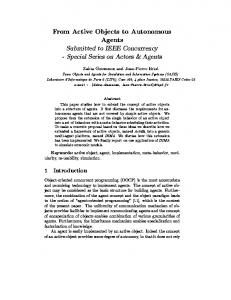
Figure 1.2: An autonomous modeling system, which consists of an eye-in-hand robot-sensor system and is utilized in this thesis, acquires a 3D model of a camel bust.

of a range sensor and pose estimation. During manual scanning, the human operator needs to plan the views and paths for the range sensor, and decide when the model is complete based on visual feedback of the acquired 3D model. In order to perform the same task as a human, autonomous modeling demands a tight coupling of 3D modeling methods with autonomous view planning and collision-free path planning. Fig. 1.2 gives an example for an autonomous modeling system which consists of an eye-in-hand robot-sensor system and is utilized in this thesis. When the sensor is attached to the robot’s end effector, the configuration is denoted eye-in-hand. In contrast to most sensor-based robotic approaches, which view the world at a distance, autonomous modeling requires interaction with the real physical world by moving into the unknown scene. It involves a robot-in-the-loop for range measurement, raw data integration into 3D models, planning of a Next-Best-View (NBV) based on a partial 3D model and moving the robot along the planned trajectory without collision. The term Next-Best-View, originally introduced by Connolly (1985), describes a sensor viewpoint which provides the best sensory input for a given task. In addition, for efficiency an autonomous system would need to measure the 3D model quality in each iteration and decide to abort if the desired quality which depends on the application is reached. For instance, object recognition still performs well if the models are accurate but not nearly complete (Kriegel et al., 2013a). In con-

1.2. CONTRIBUTION OF THE THESIS

5

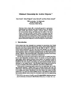
Figure 1.3: Comparison of the performance of KinectFusion with our autonomous modeling system on a pneumatic filter (left box) and a bunny (right box) object. In each box from left to right: picture of object, mesh generated with KinectFusion and mesh created with the autonomous modeling approach suggested in this thesis. For KinectFusion, the details in the objects are lost and also the object proportions are incorrect.

trast, non-adaptive grasp planning requires models with high coverage (Sahbani et al., 2012). Nevertheless, most applications that rely on 3D models perform better if the models are accurate and complete. As can be seen in Fig. 1.3, our autonomous modeling system generates object models with significantly higher quality than when using e.g. KinectFusion (Izadi et al., 2011). Obviously, autonomous view planning does not only make the model quality measurable but also saves a lot of time as Levoy et al. (2000) point out during their digitization procedure of several Michelangelo statues: “Since we did not have an automated view planning system, we planned scans by eye - a slow and error-prone process. We often spent hours positioning the gantry in fruitless attempts to fill holes in our model of the David. A view planner might have saved 25 % of the man-hours we spent in the museum.”

1.2

Contribution of the Thesis

This thesis presents an active scene exploration framework, which incorporates view planning for multi-view object recognition, exploration, and modeling of unknown objects. Thereby, it focuses on the autonomous object modeling part. Here, a scene can consist of several objects, which are either known or unknown to the robot. To accomplish efficient and accurate scene exploration, a novel approach to autonomous object modeling is introduced that emerges from the current State of the Art (see Chapter 2). The lack of current autonomous object modeling systems can be seen by the many aspects that are not yet addressed as shown in Section 2.5. Our framework incorporates all the aspects listed in Tab. 2.2 on page 27 and additionally it addresses and evaluates the

6


efficiency of the system in fast acquisition of high quality 3D surface models. Our system utilizes state-of-the-art sensors and aims at acquiring 3D models that are particularly accurate and complete. For accurate autonomous modeling, a viewpoint simplification is introduced that is not restricted to a sphere or cylinder but is directly planned based on the partially known object surface. This allows for optimally adjusting the sensor to object distance. Most general NBV algorithms try to minimize the number of necessary views to fulfill the task. In the context of 3D modeling, however, it is more important to generate a 3D surface model with a certain quality. Therefore, we introduce a quality criterion which is based on a triangle mesh and is used for NBV selection and as a termination criterion. During the NBV planning, not only a mesh but also a probabilistic voxel space is required, since exploration of the unknown area is also regarded. The key contributions of this thesis are: • A tight integration of the developed autonomous object modeling approach with object recognition methods enabling active scene exploration. Thereby, unknown objects are autonomously modeled and an object database is automatically extended by the novel object models without manual interaction. The updated database is directly applied for object recognition, which is enhanced by combining knowledge from multiple views, improving the pose estimates and avoiding object ambiguities and occlusions. • The integration of surface reconstruction and probabilistic space update, local model registration, NBV planning, exploration, and collision-free motion planning into a unified framework allows for the completely autonomous generation of object models. Furthermore, the process of autonomous object modeling is improved concerning speed, model completeness and accuracy. • A novel method for viewpoint candidate generation is developed that allows for autonomous modeling of arbitrary objects. In contrast to current state-of-the-art methods, which select NBV based on a cylinder or sphere search space, it searches for viewpoints locally based on the actual object shape of the current 3D model, considering both constant and irregular surface trend development. The method, which is called Boundary Search, is extended by hole detection once a rough model is generated and enables scan path calculation, allowing for the use of line range sensors in an intelligent way. Moreover, the environment is also considered allowing for

1.2. CONTRIBUTION OF THE THESIS

7

view occlusion and obstacle collision avoidance. • A definition of surface features improves the quality of previously scanned areas together with the exploration of unknown areas. This is achieved by the selection of NBVs based on both, the surface model quality and highest expected information gain, combining local and global information. Additionally, the system autonomously terminates when the required quality is reached. This allows for the generation of surface models with defined quality, speeding up the process e.g. for cases where a complete, highquality object model is not needed. The approaches are implemented on different robot-sensor systems and applied to real world scenarios. Thereby, the methods are first evaluated on single objects and, second, extended for active scene exploration (see Fig. 1.4). For the single object modeling, multiple sensors are integrated to allow for geometry and texture information gathering. Furthermore, objects are moved to a different orientation in order to register the model and continue scanning the bottom part.

Figure 1.4: Active scene exploration for an example tabletop scene. Top left: scene with 7 household objects. Top right: probabilistic voxel space from multiple measurements. The probabilities are color coded from black (almost free), through gray (unknown) to white (occupied). Free space is transparent. Bottom left: intermediate scene with recognized objects. Bottom right: NBV planning and modeling. The two previously occluded objects (purple) are successfully detected from this view. The flat box remains unknown and is autonomously modeled. The lines show scan path candidates generated from its partial mesh (blue) and their rating (red: low, green: high).

8


For scene exploration, known objects are recognized, the initially unknown scene is explored, occlusions by other objects are considered, and collision-free motions are planned. The object scene is segmented and the clusters are attempted to be matched with object models from a database. As object recognition sometimes results in incorrect matches, the pose is validated by its conformity to the global knowledge of the explored voxel space. If no object model can successfully be matched to a cluster, it is assumed that the object is unknown. Then, the unknown objects are autonomously modeled within the object scene using the probabilistic voxel space to plan NBVs and collision-free motions. After the desired quality is reached, the autonomously generated object models are added to the database and can be directly utilized during object recognition in future iterations. The proof of concept is demonstrated by simulations and real experiments on an industrial and a mobile robot.

1.3

Outline of the Thesis

The remainder of this thesis is organized as follows: Chapter 2 summarizes the current State of the Art regarding 3D acquisition systems, autonomous object modeling, view planning for object modeling, mapping, and exploration. Thereby, range sensors and pose estimation techniques are compared, the need for quality-oriented NBV planning is elaborated, and probabilistic 3D representations are discussed. Furthermore, the main limitations of current autonomous object modeling systems are identified and considered for the development of a novel approach. Chapter 3 gives a System and Module Overview of the proposed active scene exploration system together with the essential modules that it requires. The requirements concerning the range and pose sensors for the robot-sensor system and the used sensor calibration techniques are discussed. The motion planning of the robot based on the probabilistic model and the local registration of range images for minimizing pose error are depicted. The applied 3D model representations, a triangle mesh and a probabilistic voxel space, are defined and their real-time update is described. Moreover, the geometry-based object recognition method and the object pose estimate validation based on the probabilistic voxel space are presented. Chapter 4 describes the implemented Next-Best-View Planning for Modeling of unknown objects. Thereby, NBV candidates are planned based on the partial triangle mesh and an NBV is selected based on potential information gain of the voxel space and novel surface quality features. In a simulation

1.3. OUTLINE OF THE THESIS

9

environment, the performance of the novel NBV algorithm is compared with state-of-the-art methods based on an NBV benchmark object. Subsequently, the suggested autonomous modeling approach is evaluated in Experiments and Applications on an industrial and a mobile robot in Chapter 5. Thereby, 3D models of several hand-sized objects, but also of larger workspaces, are obtained. The model quality is assessed by comparison with ground truth models, by their application to object pose estimation, and to motion planning. The NBV planning approach is applied to different configurations: the robot moves around the object and the object is grasped by the robot and moved in front of the range sensor. Furthermore, the performance of the complete active scene exploration system incorporating object recognition and modeling is demonstrated with household and industrial object scenes. Chapter 6 summarizes and gives a Conclusion of the thesis. Further, an outlook on future work is provided.

10


2

State of the Art

This chapter covers the current State of the Art of autonomous 3D object modeling, taking related fields of research into account. Thereby, an overview of 3D data acquisition systems consisting of range sensors and pose estimation techniques is given in the context of manual and autonomous object modeling. As discussed in the previous chapter, an autonomous modeling system requires NBV planning. NBV planning is utilized in a variety of applications such as exploration, object modeling, inspection or recognition (Chen et al., 2008, 2011). However, here NBV planning is mainly discussed in the context of object modeling but also depicted for exploration. Thereby, real robotic systems which integrate NBV algorithms for autonomous object modeling are compared. The difference between surface-based, volumetric, and global NBV methods for modeling is examined and the need for a quality-oriented NBV approach is elaborated. Furthermore, NBV algorithms for mapping and exploration of unknown environments are reviewed in the context of industrial and mobile robotics. For this purpose, various 3D representations, which are based on a probabilistic approach, have been developed. These are also discussed as such a representation (see Section 3.3.2) is used for our autonomous object modeling approach. This chapter closes with a discussion on the main limitations of current autonomous object modeling methods. This thesis addresses the problems of current research, with the goal to create accurate and complete 3D models. 11

12

CHAPTER 2. STATE OF THE ART

2.1

3D Data Acquisition

3D data acquisition systems are utilized to analyze shape and possibly color from real world objects or environments and collect the data. Thereby, range sensing concepts measure the distance information and pose estimation approaches acquire the pose of the sensor with respect to a world coordinate system. In the following, different range sensing and pose estimation techniques are compared.

2.1.1

Range Sensing

Various approaches for contactless measurement of distances exist. In this work, only optical range sensors are considered, as non-optical methods, such as sonar and radar, although they provide depth information in an inexpensive way, lack of accuracy in the measurement direction. Furthermore, optical range sensors differ in their physical measurement technique. The most common systems are based on structured light, Time-of-Flight (ToF), active or passive triangulation (Blais, 2004). For structured light systems, a predefined light pattern is projected onto a scene and simultaneously observed by a camera (Zhang et al., 2002; Scharstein and Szeliski, 2003; Geng, 2011). The affordable and thus widely-used active RGBD (Red, Green, Blue plus Depth) cameras, such as the Microsoft Kinect Asus Xtion

2,

1

or

use an infrared sensor to infer depth from the deformation of a

projected speckle pattern and an RGB (Red, Green, Blue) camera to match color information to the range image. For details on the working principle of RGBD cameras see (Han et al., 2013) and for a review on its various applications see (Berger et al., 2013). ToF sensors measure the absolute time (phase delay) between emitting a light pulse and receiving its reflection. They require precise calibration and noise reduction for accurate depth measurements (Fuchs, 2012), since the measurement of returned light pulse is inexact due to light scattering and multipath mitigation. For a detailed review of ToF sensors see (Foix et al., 2011). Triangulation-based systems, which can be divided into active and passive, measure the distance by determining the size of a triangle, which is formed by two non-parallel rays viewing the same point (Hartley and Zisserman, 2003). For passive triangulation systems, the triangle consists of the two rays of a camera pair, a so-called stereo camera. The method to match the reflected light of the global illumination in both images is referred to as stereo matching. The 1 2

Microsoft Kinect http://www.microsoft.com, 2014 Asus Xtion Pro Live http://www.asus.com, 2014

13

2.1. 3D DATA ACQUISITION

Table 2.1: Comparison of different range sensors (stereo camera, RGB-D camera, ToF sensor and laser stripe profiler) in the context of 3D modeling: accuracy refers to the precision of the depth measurement and robustness refers to how well the sensor performs under changing conditions such as illumination and on untextured surfaces. The sensors are rated by best (++), good (+), bad (-) and worst (- -) suitability for each category.

Resolution Data Rate High Illumination Low Illumination Untextured Surfaces Accuracy

Stereo ++ ++ ++ ---

RGB-D ++ + -+ ++ -

ToF + + + ++ --

Laser --+ ++ ++ ++

distance between the two cameras is referred to as base distance. For active triangulation systems which contain a light source, the ray of the light source to the intersected surface point and the reflected ray captured by an optical camera form the triangle. Structured-light sensors are also based on the active triangulation principle and laser triangulation systems can also be categorized as structured-light systems since a laser stripe or point also represent patterns. Nevertheless, these are treated separately here. In the area of laser triangulation, we only consider laser stripe profilers such as presented by Winkelbach et al. (2006) and Suppa et al. (2007). Here, laser light illuminates a stripe when colliding with the object surface recording the reflection with a camera. Laser stripers obtain high quality depth measurements, but only acquire a 1D range image. More recently, laser range scanners have been developed which allow for a variable range due to an autofocus camera (Kielhöfer et al., 2011). However, the application to 3D modeling still needs to be evaluated. In Tab. 2.1 the different range sensor types (stereo camera, RGB-D camera, ToF sensor and laser stripe profiler) are compared in the context of 3D acquisition concerning range image resolution, frame rate, measurement accuracy and system robustness. The resolution is defined by the size of the range image which represents a matrix or stripe of depth values. The data rate relates to the amount of depth values per time segment. High illumination refers to very bright scenarios such as outside or a room with sunlight coming in whereas low illumination refers to dark areas. Untextured surfaces describe object surfaces with no texture as in several industrial objects. Accuracy refers to the absolute measurement error of the sensor. The sensors are rated by best (++), good (+), bad (-) and worst (- -) suitability for each category. However, as several examples for each range sensor type exist, this categorization only describes an

14


estimation but might not be correct for each model. A stereo system is not very robust against low illumination, as no active illumination is given. Furthermore, stereo cannot measure untextured surfaces as the measurement principle depends on the corresponding feature. However, this disadvantage can be compensated by using a pattern projector in addition to the passive stereo system. Stereo cameras are very flexible as the base distance and the camera type and therefore working range and resolution can be adjusted depending on the application. Nevertheless, higher resolution does not allow for real-time range image acquisition as is the case for the other sensors. In order to acquire near real-time stereo reconstruction, the algorithms need to be ported to GPU (Graphics Processing Unit) or FPGA (Field Programmable Gate Array) boards. In (Gehrig et al., 2009) an FPGA implementation of the Semi-Global Matching (SGM) algorithm (Hirschmüller, 2008) is presented. The suggested system allows for real-time range image acquisition with VGA (Video Graphics Array) resolution. RGB-D cameras also generate range images with VGA resolution, ToF cameras only below QVGA (Quarter Video Graphics Array) and laser stripers simply deliver a 1D range image. A major drawback of the laser striper is that the acquisition of a complete view of an object requires time, since the laser stripe needs to be moved over the object. RGB-D sensors catalyzed a multitude of efforts for 3D modeling and recognition due to the low-cost. Despite its indisputable uses, the work of Meister et al. (2012) shows that for 3D reconstruction of objects, curved and concave details in the scale of around 10 mm are lost and simply smoothed out. This indicates that only with laser sensors accurate depth measurements can be generated. In (Smisek et al., 2011), the accuracy of stereo, ToF and Kinect systems is compared. Stereo and Kinect perform similar and the ToF sensor generates the most inaccurate range images. However, the ToF does not seem to be calibrated correctly and noise reduction is not considered. Stoyanov et al. (2011) also compare Kinect and two ToF sensors with a laser sensor, which is used as ground truth. In their evaluation, the Kinect is slightly better than the two ToF but the difference in accuracy is minor. In some robotic applications such as for flying robots, the weight and power consumption of the sensor is an issue. Stereo cameras can be very light and RGB-D cameras are also light. ToF and laser sensors are both rather heavy. Although RGB-D sensors are light, their shape is not very reasonable for attaching it to the hand of a robot. The working range is also of interest as it presents the depth area in which measurements can be obtained. The working range of the Kinect is more limited than for ToF cameras. For stereo systems

15

2.1. 3D DATA ACQUISITION

it is adjustable as mentioned before. The high accuracy of laser striper systems comes at the cost of a very narrow working range. Other robotic applications might also be considered to work outdoors or both outdoor/indoor for example in case of a mobile robot. In general, stereo systems work better in outdoor scenarios (Schmid et al., 2012) as they depend on the global illumination. Outdoors, ToF sensors perform well (Langmann et al., 2012), whereas RGB-D cameras have difficulties with direct sunlight and heated surfaces (Mura et al., 2012). In this thesis, we will refer to ToF, RGB-D and stereo sensors as aerial 3D sensors. In contrast to laser stripers, these obtain a matrix of distances which represents a larger area of the environment and not simply a line.

2.1.2

Pose Estimation

When range images are obtained from different viewpoints, as is needed for complete object modeling, the sensor pose is required for alignment of the acquired data. Pose estimation can be performed with optical tracking systems, passive measuring arms, robotic manipulators or by the range sensor itself. For optical tracking systems, passive or active markers are attached to the object, which is then tracked with optical cameras. They allow for a large working area depending on the size of the room at the cost of accuracy. In contrast, passive measuring arms restrict the working area very much but measure highly accurate poses. Nowadays, a range sensor in combination with a passive measuring arm is usually used for accurate 3D modeling. In this work, a Faro Platinum measurement arm

3

in combination with a Nikon ModelMaker D

4

as

in Fig. 2.1(a) is used to generate ground truth 3D models. Robotic manipulators can be used for both handheld or autonomous sensor placement.

Various platforms such as industrial, light-weight or humanoid

robots with varying accuracy are available to which range sensors can be attached. However, for all these robots, the positioning accuracy is not as accurate as for passive measuring arms. Alternatively, algorithms that estimate the pose based on the image or range data of the range sensor itself also exist. The computation of the camera motion from a sequence of images is referred to as ego-motion (Burger and Bhanu, 1990). Strobl et al. (2009) present an ego-motion system for simultaneous object modeling with a laser striper and ego-motion estimation with a stereo camera by feature tracking. The different sensors are integrated in the DLR 3D Mod3 4

Faro Platinum arm http://www.faro.com, 2014 Nikon MMDx http://www.nikonmetrology.com, 2014

16


(a) measurement arm

(b) ego-motion

Figure 2.1: Handheld 3D scanning system consisting of a Faro Platinum measurement arm and a Nikon ModelMaker D laser scanner (left) and using ego-motion for pose estimation with the DLR 3D-Modeler (Suppa et al., 2007) (right).

eler (Suppa et al., 2007). Figure Fig. 2.1(b) shows a human moving the DLR 3D Modeler around the object in order to acquire a 3D model without external pose sensor. In the work of Rusinkiewicz et al. (2002) 3D models of objects which are moved in front of a structured-light system are generated by Iterative Closest Point (ICP) alignment of the range images. A more recent application for high quality geometry reconstruction, the KinectFusion (Izadi et al., 2011), is based on the same principle but the compact sensor, the Microsoft Kinect, is not restricted to a fixed setup. Nevertheless, ego-motion also lacks pose estimation accuracy and fails if the pose is lost due to an abrupt movement of the sensor or for feature tracking if not enough features are detected. Autonomous modeling requires a robot as the object and/or sensor need to be actively moved. All the other pose estimation techniques require a human operator for moving the range sensor and therefore only allow for manual 3D modeling. As the pose of the robot is inaccurate, ego-motion estimation could be used to improve the pose measurements.

2.2

Autonomous Object Modeling

So far, little research in the area of real autonomous object modeling systems has been exercised. In the work of Kasper et al. (2012), a semi-automatic approach for 3D model generation is presented. A single object is placed on a turntable and then two sensors are consecutively moved along fixed rigs for obtaining

2.2. AUTONOMOUS OBJECT MODELING

(a) Fixed semi-automatic approach

17

(b) Automatic robotic approach

Figure 2.2: Systems which attempt to automate 3D modeling reach from large, fixed and expensive systems consisting of several sensors and rigs (left) to automatic methods incorporating an industrial robot, a turntable and a fringe projection system (right). For both, a human operator has to place or even fixate the object in the desired place. Image credits: a) (Kasper et al., 2012) b) (Khalfaoui et al., 2013)

geometry and texture information of the object. Here, object modeling requires a very large, fixed and expensive setup (see Fig. 2.2(a)) and the acquisition time of 20 minutes and 30 to 60 minutes for post-processing is quite high. Furthermore, the 3D model are noisy and still contains holes. Therefore, the model generation requires manual interaction by a human operator. A similar approach for creation of object databases has been presented by Singh et al. (2014). Here, the object modeling is performed automatically except for the placing of the object. However, the model quality is not as good as for the system of Kasper et al. (2012), since RGB-D sensors and high resolution cameras are utilized. Both systems do not allow for scanning the bottom part of an object and also view planning is not considered as the objects are of simple shape. Most NBV approaches for object modeling (see Section 2.3) suggest a method to solve the view planning problem theoretically but neglect sensor and robotic aspects and therefore do not take into account system calibration, sensor noise, robot positioning errors or workspace limitations. In the remainder of this section we want to inspect research, which applies NBV algorithms to autonomous object modeling systems consisting of real sensors and robots. In the work of Foissotte et al. (2009), 3D models of single objects are obtained with the stereo camera and a humanoid robot. The objects are placed on a table and the robot moves around the table for a complete model. However, the model quality is not evaluated as the focus lies on recognition and also the procedure is only tested in simulation. The pose reachability considering stability and collisions are evaluated on the real robot. In (Callieri et al., 2004)

18


and (Larsson and Kjellander, 2008), autonomous 3D modeling in three steps is presented using an industrial robot in combination with a turntable. First, a rough scan is performed in order to obtain only the bounding box of the object. Second, NBVs are determined based on a cylinder model and the object is scanned from several directions resulting in an approximate model containing holes. The third step performs a rescan of hole areas where no information could be obtained during the second step due to occlusions or a significantly differing line of sight and surface normal. However, Larsson et al. have not implemented the third step so far. Both systems are limited to a cylinder viewpoint space. Callieri et al. (2004) focus on 3D modeling but do not consider path planning aspects at all. In (Larsson and Kjellander, 2008), the user needs to manually input object size and stand-off distance for each object individually, which does not render the system autonomous. Karaszewski et al. (2012) present a measurement system consisting of a turntable and a vertically moveable pedestal for modeling small and large cultural heritage objects. The human needs to initialize the size of the object for which a voxel space is initialized with the state ’unknown’. Based on the depth measurements, the voxels are simply updated with ’free’ and ’used’ not considering sensor noise. Karaszewski et al. suggest that a system for 3D modeling should not depend on a robot type. In a first step areas in the boundary area and in a second step areas with low point density, are selected as viewpoint candidates. All viewpoints are simply processed without reasonable NBV selection and also no abort criterion is introduced. 3D modeling of a few cultural heritage objects is shown but the quality of them is not evaluated. The system does not seem to be optimized concerning time. For a small object, the digitization time was over 19 hours. Loriot et al. (2008) present a system with a similar setup using a fixed scanner but moving the object in order to scan it. In a first step, the method determines NBVs by the Mass Vector Chain approach (Yuan, 1995), which is very suboptimal considering the trajectory length as the NBV is in opposite direction of the main orientation of currently acquired data. In a second step, holes are determined and rescans are planned for these. The system is restricted to very small objects and aims at the development of a 3D scanner automated turntable. Furthermore, the authors do not mention any processing times and do not ensure a certain model quality. In the work of (Khalfaoui et al., 2013), an automatic 3D digitization system consisting of an industrial robot, a turntable and fringe projection system is developed (see Fig. 2.2(b)). The fringe projection system is very large and ex-

2.2. AUTONOMOUS OBJECT MODELING

19

pensive. Therefore, this system is only applicable to standalone solutions and not for robots which should perform different tasks such as modeling, recognition and grasping. For view planning, the visibility of each face is checked in the acquired surface model and well visible and barely visible surfaces (high incidence angle) are defined. Each normal of a barely visible face represents a viewpoint candidate from which an NBV is selected. For the selection mean shift clustering is performed, considering a minimal distance criterion to avoid viewpoints being too close to each other. The acquisition time for four objects with different complexity, which are automatically obtained, is between 5 and 25 min. However, several holes in the models remain, which can only be closed by a post-processing step. Also, the bottom parts of the models cannot be obtained. The automatic approach is compared with manual scanning and is faster. However, the manually acquired models are complete in contrast to the automatically acquired ones. Furthermore, the comparison should be with a hand-guided system as manually moving an industrial robot is always slower. The robot speed is significantly reduced in manual mode. Also, for a human it is almost impossible to move the robot in configuration space manually in an optimal way. Torabi and Gupta (2012a) also use a 6DOF (six-degrees-of-freedom) robot with mounted 2D range sensor. A set of points on the occlusion surface which the authors call target points are scanned. The system switches between modeling and exploration scans, in order to be able to move into initially unknown areas. However, this is similar to other methods and they do not consider improvement of the known surface. Furthermore, the viewpoint search space is still discretized by four spheres with different directions. The average post-processing time per scan iteration was 4 min, resulting in a total model acquisition time beyond 1 hour, which is also very high. Although Torabi et al. introduce a model completion criterion, both workspace scenarios are not sufficiently completed and even for a simple mug still approx. Six percent of the target points could not be eliminated. In (Torabi and Gupta, 2012b), this method is ported to a mobile robot. In the work of Krainin et al. (2011) the setup is inverted. Objects are modeled by grasping them, moving them in front of an RGB-D camera, tracking them, and planning an NBV regrasp for covering the previously occluded parts. However, only for the regrasp an NBV is planned but the robot trajectory is predefined obtaining all 3D measurements. The methods seems to work well for the test objects, which are of simple shape though and highly textured which makes tracking easier. The color matching in ICP would fail for untextured objects

20


such as occur in industrial environments. The models look very noisy, which is due to the fact that the quality of acquired 3D geometry models is very low for RGB-D cameras and could be improved with laser stripers. In the work of Aleotti et al. (2014a), an industrial robot with gripper and laser scanner is presented for modeling multiple objects in a scene by manipulation. The work does not contain view planning, as the laser scan is always a precomputed path. The objects are modeled by choosing to rotate the object by ±90 or 180 degree around the z-axis. The model quality is evaluated by comparing the dimensions of the reconstructed model with the measured object dimensions. However, no comparison with actual ground truth is performed. In (Aleotti et al., 2014b), the same authors replace the gripper with a 3D camera and apply the system to similar scenarios with multiple objects. Here, the objects are modeled by iteratively moving the 3D camera to planned NBVs based on a standard approach. The NBVs are selected from a sphere search space for each cluster which maximize the information gain of unexplored regions in the volumetric model with an overlap with previous range data. Further, a global registration is performed for matching the different range images which proved to be better than pairwise ICP. Both these papers, are the only ones which considers object scenes with multiple objects. However, the distances between the objects are very large and also the objects are hardly occluded by other objects at all. Box- and cylindrical-shape objects are used which are symmetrical and thus no complete observation of these is needed if this assumption was considered.

2.3

View Planning for Object Modeling

While the task where to position the sensor next in order to provide the best sensory inputs, is intuitive for a trained human operator, it is very complex for a robot. This problem is referred to as the view planning problem and has been addressed by several researchers since the 1980s. However, in most cases, it is not desirable to find the absolute best viewpoint as in 6DOF space an infinite number of viewpoints is possible, which cost time and memory. Therefore, usually a tradeoff between efficiency and performance is chosen by reducing the search space. Scott et al. (2003) present a good overview of model-based and non-modelbased NBV algorithms for object modeling and inspection. For model-based approaches, which are used for inspection, the views can be planned offline allowing for a quick online scanning procedure. On the contrary, for non-model-

2.3. VIEW PLANNING FOR OBJECT MODELING

21

based algorithms, an NBV needs to be selected in runtime since no a priori information about the target object is given. Here, in a greedy manner, NBVs are iteratively selected until a complete object model is generated. This problem is more complex than when a preexisting model is given (Scott et al., 2003). In the following, only non-model-based NBV algorithms are analyzed as the task of this thesis is the autonomous modeling of unknown objects. In (Scott et al., 2003) existing non-model based NBV methods are summarized and classified as volumetric, surface-based and global. The advantage of a volumetric model is that spatial information is available, which can be used for occlusion avoidance, ray casting etc. Contrary, a surface model usually describes the object shape in more detail as the volumetric model uses a lower resolution due to computation complexity. In the following, these methods are compared, the difficulties of current NBV algorithms are described and the need for efficient quality criteria during NBV planning is discussed. Surface-Based The occlusion edge principle is introduced in the work of Maver and Bajcsy (1993), Their NBV algorithm focuses on finding two different types of occlusions along the boundaries of objects by “shadow zone pixels”. In the work of García et al. (1998), a mesh is used to identify those vertices which lie at the boundary of the regions contained in the triangular mesh and refers to them as exterior vertices. A view sphere is applied onto which orientations are mapped using spherical discretization maps. In (Milroy et al., 1996), an orthogonal cross sections model is built based on the surface model and laser scans are planned perpendicular to cross sections at the boundary of the scanned surface. A similar approach, the trend surface, is suggested by Chen and Li (2005) in order to predict the unknown portion of an object, which is based on surface information and not on occlusions. The global shape of the previously scanned surface is estimated in order to determine the NBV for the expected surface. Zhou et al. (2009) also predict the surface, to the left and the right side of the visual surface and select the NBV with the larger visible surface. However, the model is restricted to a cylinder and the method does not work on objects which contain larger concave areas or occlusions. Volumetric Most volumetric methods incorporate a voxel space, which is initialized with the state “unknown”. Then, viewpoints are randomly sampled over a given search space and an NBV is selected according to the visibility criterion. The visibility criterion counts the amount of unknown voxels, which are visible from a viewpoint and chooses the one with the highest amount as

22


(a) View sphere

(b) View cylinder

Figure 2.3: In many NBV algorithms a cylinder or sphere is used as search space from which an NBV is selected. Image credits: a) (Wong et al., 1998) b) (Pito, 1999) ©1999 IEEE

NBV. The algorithm by Wong et al. (1999) method is based on this principle. The authors randomly sample viewpoints over a sphere (see Fig. 2.3(a)), which circumscribes the unknown object. Wong et al. additionally implemented a surface normal and adaptive variant, which speeds up the process but does not improve the model quality. The work of Blaer and Allen (2007) is based on the same principle with the difference, that a 2D map instead of a sphere is used for site modeling of a fort and church with a mobile robot. In (Banta et al., 2000), three NBV algorithms are integrated into one large system giving voxels the status occupied or unoccupied. This approach incrementally iterates over a sphere and verifies the status of the voxels from the candidate viewpoint direction. Global The global methods determine an NBV from global rather than local geometric shape information. However, these could also be classified as surface-based as they also use surface information. In (Yuan, 1995), a Mass Vector Chain approach is proposed for planning the NBV. A Gaussian mass sum over all surface normals is calculated, which results in an NBV pointing toward areas where unprocessed surface patches are assumed. However, the method cannot handle holes due to self-occlusions. In the work of Pito (1999), the occlusion-based concept of “positional space” is introduced as a basis for visibility representation of the object surface and the sensor ability. A cylinder (see Fig. 2.3(b)) circumscribes the object, which is partitioned into three types of information, recovered from range data: the void volume, the void surface and the seen surface. Thereby, overlap constraints are considered but the computational complexity is not addressed. Trummer et al. (2010) determine

2.3. VIEW PLANNING FOR OBJECT MODELING

23

a covariance matrix for every measured 3D point. An NBV is chosen for the point with the largest eigenvalue and calculated orthogonal to the corresponding eigenvector. This represents the largest directional uncertainty over a sphere. However, the authors do not consider self-occlusions or model completeness. Difficulties For all NBV algorithms, a simplification of the 6DOF space is required in order to perform NBV planning in reasonable time. Most nonmodel based NBV algorithms for object modeling restrict the search space of the viewpoints to a cylinder or sphere model. Thereby the candidate views always point to the center of the cylinder or sphere reducing the problem from six to two degrees of freedom. This makes it impossible to view all the surfaces of objects with complex geometry. Therefore, a cylinder or sphere search space is only optimal if the object itself is of cylindrical or spherical shape. There is a need for a search space simplification which is not predefined but adapts to the actual object shape. Quality Criteria It is very difficult to give a measure for the quality of a reconstructed object if no ground truth is given. That is probably the reason why very little research (Massios and Fisher, 1998; Albalate et al., 2002; Vasquez-Gomez et al., 2009) also considers model quality while planning the NBV for an unknown object. These approaches are all based on a volumetric model. Massios and Fisher (1998) were the first that used a quality criterion in addition to the visibility criterion in a utility function, aiming at improving the quality of the surface. The angle of incidence (the angle between surface normal and viewing direction) is determined for each voxel and used as surface quality criterion assuming to improve voxels which were seen at a bad angle. However, the viewpoints generated over a tessellated sphere are constrained. Only views on a circular arc with 10◦ steps were utilized in the experiments. The authors do not prove that by using the quality criterion a better 3D surface model quality is reached than without. In (Vasquez-Gomez et al., 2009), the same quality criterion is used in the utility function and extended by traveling distance and overlap with previous range images. Here, 80 candidate views are sampled over a sphere starting at a low ray tracing solution and then evaluating the best views with a higher resolution. This is done to speed up the process and is described in detail in (Vasquez-Gomez et al., 2013). In (Vasquez-Gomez et al., 2014a), the same authors apply their algorithm to a mobile robot and plan views directly in configuration space. However, the experiments on the real robot are only briefly described and no actual surface model of the object

24


is generated. The work of Albalate et al. (2002) also uses viewing angle and overlap but not traveling distance as quality criterion. It seems intuitive that a low angle of incidence leads to more accurate depth information. However, these authors do not prove that this really leads to a better reconstructed model quality. According to (Mehdi-Souzani et al., 2006), when using real laser scanners, the quality of the reconstructed surface does not differ significantly if the angle of incidence is below a threshold around 60◦ but then increases enormously. In (Scheibe et al., 2006; Bodenmüller, 2009) similar observations have been made with two laser scanners with completely different working ranges. However, if the angle of incidence is higher than a cut-off angle, the quality of the 3D model decreases significantly. One reason for this is that range data with a flat lineof-sight onto the surface in combination with noisy measurements cause wrong decisions on the sign of the estimated surface normal. Johnson et al. (1997) also investigate the measurement error for different angles of incidence and find out that the error is constant up to a certain angle. Therefore, vertices with a certain cut-off angle are removed in the mesh. Therefore, the angle of incidence should be used as quality criterion but only as a binary. Nevertheless, as you can also see in (Suppa et al., 2007), the surface to sensor distance also plays a very important role for laser scanners and should also be considered as quality criterion. The evaluation of Scheibe et al. (2006) shows that the 3D point quality depends a lot more on distance than on angle of incidence. In (Prieto et al., 2003) also distance and incidence angle both are considered as important factor for laser scan quality. However, if the search space is restricted to a sphere like in the work mentioned early, then distance cannot be considered since it is already predefined by the sphere and is only optimal if the object is evenly sized. Therefore, a viewpoint space is required where the distance is not fixed.

2.4

Mapping and Exploration

In the area of mobile robotics, optimal robot positions are required for efficient exploration of unknown environments. In order to apply information gain driven exploration, metric grid maps are used. Several mapping methods that integrate range data into a voxelmap have been presented (Thrun et al., 2005). In contrast to a stationary robot, a mobile robot needs to build a map of its environment and localize itself within the map by active perception before a next-best robot position can be planned. This problem is known as simultaneous localization and mapping (SLAM) and has been addressed by many

2.4. MAPPING AND EXPLORATION

25

researchers (González-Baños and Latombe, 2002; Durrant-Whyte and Bailey, 2006; Nüchter and Hertzberg, 2008). The two key solutions to solve the SLAM problem make use of the extended Kalman filter (Dissanayake et al., 2001) and the Rao-Blackwellized particle filters (Montemerlo et al., 2002). However, SLAM does not consider the problem of where the robot should go next. This problem is similar to the NBV problem (see previous section), but aims at exploration of unknown environments and not modeling of unknown objects. In (González-Baños and Latombe, 2002), safe-regions for a mobile robot are defined within the current map. A next robot position is iteratively selected within the safe region, which maximizes the information gain considering an overlap with the global map. The frontier-based approach presented by Yamauchi (1997), is a well-known concept which explores the environment by planning robot positions on the frontier between free and unknown space. This is similar to the occlusion edge principle (Maver and Bajcsy, 1993) for object modeling. The frontier-based approach has been extended by several researchers (González-Baños and Latombe, 2002; Freda and Oriolo, 2008) and used in a variety of applications such as in (Blodow et al., 2011) for planning positions of a mobile robot in order to explore a complete room. In the work of Oriolo et al. (2004), the Sensor-based Random Tree (SRT) method, a sensorbased version of the rapidly-exploring random tree (RRT) method (Kuffner and LaValle, 2000) used for path planning, is introduced. SRT represents a roadmap of explored areas with local safe regions associated to each node, providing an estimate of the surrounding free space for each configuration. However, the SRT method only works for disc shaped robots. The next robot positions are iteratively chosen by sampling random directions from the current configuration and selecting a new configuration which is at least a certain distance away and is still within the safe region. Here, only a 2D map is obtained and the problem of localization is not considered. In (Low and Lastra, 2006), 3D models of larger environments are obtained using a mobile platform with a 360 degree scanner. The authors introduce a hierarchical NBV algorithm by grouping neighboring views into view volumes and neighboring surface points into surfaces patches. Then they evaluate the view metric for the groups and perform a subdivision (if required) which finally leads into an NBV. Although here a 3D map of the environment is obtained, it is assumed that the robot always moves on one level. Therefore, the viewpoint space is only a 3DOF problem in contrast to NBV planning for object modeling. Therefore, these approaches do not seem to work in feasible time if a 6DOF problem is given. With a 2D map, the robot is restricted to moving around but cannot perceive

26


(a) Table scene

(b) Outdoor map

Figure 2.4: Probabilistic 3D representations are used in a variety of applications such as exploration of table scenes with industrial robots (left) or mapping of larger outdoor environments with mobile robots (right). Image credits: a) (Suppa, 2008) b) (Hornung et al., 2013)

or manipulate objects on a table. Therefore, for complex robotic tasks, localization within a 3D map of the environment is required, which is referred to by 6D SLAM (Nüchter, 2009). Thus, efficient 3D representations and methods to update the model by sensing have been developed in the field of SLAM and exploration. An efficient approach to 3D mapping, the OctoMap, has been proposed by Wurm et al. (2010) and advanced by Hornung et al. (2013), who also give a more detailed overview of the literature. The map is a volumetric model based on octrees and uses probabilistic occupancy estimation. For details on octree data structures see (Samet, 1990). A very similar mapping approach has been proposed earlier in the context of work cell exploration with an industrial robot (Suppa, 2008). In contrast to OctoMap, distant-dependent noise is considered during ray tracing. In the work of Suppa, different probabilistic update strategies for beam-based mapping relying on depth measurements are compared. The necessity to consider sensor uncertainty is demonstrated and a probabilistic approach which interprets the sensor data is utilized. Well-known 2D-mapping techniques as in (Thrun et al., 2005) are introduced to 3D. Suppa gives a detailed survey of update-strategies and their application in the context of autonomous robot work cell exploration. Furthermore, a preliminary approach how to integrate NBV planning for exploration and 3D modeling is shown. Suppa proposes to use a Bayesian update rule for voxels. The work of Potthast and Sukhatme (2011) shows that a Bayesian space update proved to be faster than using a simple approach for exploration of cluttered scenes. The authors utilized a humanoid robot and an eye-in-hand camera in their evaluation. Probabilistic 3D volumetric models are applied in various fields such as localization, mapping, 3D modeling and exploration. For instance, the models are used for exploration of a table scenes with an industrial robots (see Fig. 2.4(a)) or mapping of larger outdoor environments with mobile robots (see Fig. 2.4(b)).

27

2.5. SUMMARY AND DISCUSSION

2.5

Summary and Discussion

Here, the most important systems for autonomous object modeling of unknown objects presented in Section 2.2 are summarized and compared in Tab. 2.2. The

Callieri et al. Larsson and Kjellander Karaszewski et al. Loriot et al. Khalfaoui et al. Torabi and Gupta Krainin et al. Aleotti et al.

x x x x

x x x x

Completeness Check

Exploration

Accuracy Planning

Multiple Object Scene

Complete Models

Texture

Range of Objects

Volumetric Model

Surface Model

Table 2.2: Comparison of autonomous object modeling systems

x x x x

x x x

x

x x

aspects refer to the kind of model utilized, the object characteristics, and active sensing techniques applied. As described in Section 2.3, NBV algorithms are categorized as surface-based, volumetric and global. Here, we only distinguish between the kind of model that is used. Thus, global NBV methods are categorized as systems based on a surface model. The advantage of a volumetric model is that spatial information is available which allows for direct access of certain areas and instant ray tracing. However, a surface model, which is the desired output for most applications, incorporates information on the quality and accuracy of the surface shape. Thus, it would be beneficial to use both models when planning an NBV which is not the case for the state-of-the-art systems. Other model representations such as topological models also exist but do not aid the NBV planning. Only three systems consider objects from different application domains. None of the approaches except for (Krainin et al., 2011), obtains texture and a complete model of the object. Both of this information, is required e.g. for texture-based object recognition or if the objects are placed on different sides as is the case in a real world scenario. None of the state-of-the-art object modeling methods

28


consider the accuracy, namely of the surface model, during the view planning or verify the actual object completeness in the surface model. Therefore, the quality of the acquired models cannot be evaluated or assured. This is mandatory if the object models should be directly applied to another application such as object recognition or manipulation without manual interaction. None of the methods show the applicability of the generated 3D models. Some of the presented work does not even generate a 3D model but simply outputs a point cloud, which could be too noisy for a reasonable surface model. Furthermore, most methods reduce the 6DOF search space to a box, sphere or cylinder. If the search space is restricted suchlike, then for complex shapes not all areas of the object can be scanned. In these cases, the object models cannot be completed. Callieri et al. (2004), Karaszewski et al. (2012), and Loriot et al. (2008) try to acquire complete models by rescanning holes but do not consider the bottom part of the object. Moreover, for most methods the acquisition time of 3D models is very long. For all methods the object needs to be manually placed in the correct position and object modeling of unknown objects within a scene consisting of multiple objects is only considered by Aleotti et al. (2014a). This is desirable if a robot needs to learn new objects itself which it encounters in a real scenario such as on a table or in a shelf and there is no human, who can get the object for the robot. Furthermore, none of the state-of-the-art approaches combines object recognition and autonomous object modeling. In this thesis, we present an approach for autonomous modeling of unknown objects within a scene and thereby incorporate all the aspects listed in Tab. 2.2. Furthermore, the autonomous object modeling is combined with active object recognition for a better scene understanding. An overview of the system is given in the following chapter.

3

System and Module Overview

This chapter gives an overview to the active scene exploration system and describes its essential modules. The modules do not describe new research and have mainly been presented by others. However, the novel methods (see Chapter 4) developed in this thesis require understanding of the basic modules, which have been extended and combined into a unified robot-sensor system to achieve autonomous object modeling and active scene exploration. The basic modules include sensor calibration, motion planning, pose error minimization, 3D model generation, and object recognition and validation. The context of these modules within the scene exploration concept is given in the following section.

3.1

Overview

In the following, the procedure for active scene exploration is described in detail. Active scene exploration denotes the exploration of an initially unknown object scene by active recognition of objects for which a model is given and autonomous modeling of unknown objects. Fig. 3.1 gives an overview of the suggested modules and concepts which tightly integrate active object recognition and autonomous object modeling. However, the focus of this thesis lies on the autonomous modeling part (right bounding box). For an example scene, the different steps during scene exploration are depicted in Fig. 1.4 on page 7. 29

30 CHAPTER 3. SYSTEM AND MODULE OVERVIEW

Figure 3.1: Overview of active scene exploration concept: active object recognition and autonomous object modeling are tightly integrated for exploration of complete object scenes with a robot-sensor system. The detection of unmatchable data clusters during recognition triggers the modeling of unknown objects and a database update. This thesis focuses on the autonomous object modeling part (right bounding box). Yellow boxes represent modules, blue diamond boxes decisions and purple ovals robot-sensor system actions. For the modules, the section (Sec) or chapter (Ch) in which it is described in this thesis is stated.

3.1. OVERVIEW

31

Active scene exploration requires a robotic system and 3D range sensors which is elaborated in Section 3.2. For quick overview range images and more accurate models, different range sensors, a laser striper and an aerial 3D sensor, are combined. As the 3D sensors are usually attached at the robot’s flange, the system requires hand-eye calibration, in order to merge the range and pose data into globally aligned 3D points. The sensor calibration of aerial 3D sensors and laser stripers used in this work, is detailed in Section 3.2.1. For exploring partially unknown object scenes, initially an overview range image with the aerial 3D sensor is obtained from a random position on a half sphere enclosing the complete object scene. The dominant plane of the tabletop is detected using RANSAC (Random Sample Consensus). The resulting point cloud is segmented by plane subtraction and Euclidean clustering. For each cluster, a geometry-based object recognition (see Section 3.4) is performed using an object model database. The database contains a set of a priori known object models. If the quality of the highest object hypothesis is sufficient, the object is considered to be correctly recognized. Then, the candidates are validated through their conformity to the global knowledge of the explored voxel space. Fig. 1.4 on page 7 bottom left depicts an example where for the initial view only the green objects are successfully recognized. If no object model can be matched to a certain cluster, it is assumed that the object represented by this cluster is unknown. Then, the autonomous object modeling is triggered. Here, the only difference to modeling single objects (see Chapter 5) is that other objects might be in the way. In order to plan NBVs for object modeling, information of the surface shape and the borderline between occupied and free space is required. As a point cloud does not describe this information directly, further 3D model representations are needed. Therefore, based on the 3D measurements, a triangle mesh and a probabilistic voxel space (PVS) are generated, which is described in Section 3.3. The PVS (see Fig. 1.4 on page 7 top right for an example) is initialized for the dominant plane of the scene. As the triangle mesh is the desired output representing the initially unknown object, it is updated only for the 3D points within a bounding box defined by the unknown cluster. A local registration (see Section 3.2.3) is performed for minimizing the robot pose error of the 3D points assigned to the cluster. It is mandatory for accurate 3D modeling due to the robot and calibration inaccuracy. Registration refers to fine matching of different partial 3D models. Local registration implies that two partial models obtained from different views are locally merged. After the registration, using only the PVS information within the cluster’s bounding box, NBVs are iteratively planned (see Chapter 4),

32

CHAPTER 3. SYSTEM AND MODULE OVERVIEW

collision-free motions are determined (see Section 3.2.2), and range images are obtained until the desired model quality is reached. The collision-free motions are planned based on the known environment and the constantly updated PVS. Furthermore, the model quality requirements are evaluated in each planning step and considered during the NBV planning. Thus, the surface features of the triangle mesh and the PVS are fused into a single space as described in Section 4.5.1. Fig. 1.4 on page 7 bottom right shows the partial mesh for a flat box (blue), for which no object model is given, and the scan path candidates with corresponding rating, which are color coded from low (red) to high (green). A more detailed overview of the actual NBV planning algorithm is given in the following chapter. The local registration, mesh generation and PVS update have been briefly presented by Kriegel et al. (2013b) but are described in more detail here. Additionally, for each unknown cluster, the object recognition is repeated with the aerial 3D sensor during the first laser scans to ensure that the object model does not already exist. This could be the case if it has not been correctly recognized in previous steps e.g. due to occlusion or false object recognition. For the object pose estimation, NBVs are planned using the same NBV algorithm originally presented for modeling (see Chapter 4) in order improve the recognition by gaining more information of the scene from multiple views. As the scene is continuously explored and updated considering sensor uncertainties, the robot can move into the initially unknown workspace (see Fig. 1.4 top left for an example). This is required as it will not always be possible to view all parts of an object from views outside the scene due to occlusions by other objects. After an object model of an unknown object is autonomously generated, it is automatically added to the object model database. For each model, the database holds its currently estimated location as a bounding box computed from the range image, and a merged triangulated model from the high quality laser scans. Thus, the new model is directly applied for pose estimation in further iterations. The algorithm aborts when no unknown clusters remain which means that for each cluster an object from the database could be matched. Here, we assume that the unknown objects are separated in the scene which means that they are at least a few millimeters apart. Otherwise, an object model could be created which can contain information of both objects, as for this case the segmentation is not successful. Furthermore, no object should be totally occluded. Otherwise it is not possible to acquire any 3D data of this object.

3.2. ROBOT-SENSOR SYSTEM

3.2

33

Robot-Sensor System

Concerning the robot-sensor setup, for the range sensor two placements on the robot are possible: eye-in-hand or external. For eye-in-hand configuration, the robot needs to be moved in order to model the object. As presented in Section 2.2, most autonomous modeling methods use a turntable in addition to the eye-in-hand robot. This is not an option for our robotic system as it is required to model several objects within one scene without the need of a human to place each object on a turntable. Furthermore, a turntable limits the object size. However, for fixed eye-in-hand robots without turntable, the workspace limitations need to be addressed more carefully as objects will only be viewable from all sides in a certain area. Therefore, the optimal object position needs to be determined. If the sensor is externally mounted, then a robot needs to grasp the object and move it in front of a sensor in order to completely reconstruct it. An external configuration may be required if the object is placed in the world so that it cannot be viewed all around due to the robot arm workspace restrictions. For instance, if a mobile robot navigates within everyday environments, objects on a table or shelf may be reachable but cannot be viewed from behind. As for both cases, the robot is moved to view different parts of the object, the model reconstruction quality depends on the accuracy of the sensor and the robot. Although there are methods for improving noisy data and range image misalignment (see Section 3.2.3), the model quality will always be limited by the hardware and therefore the robot-sensor system needs to be chosen carefully depending on the application and desired output. Furthermore, only one or several sensors can be applied. For active scene exploration, it is advantageous to create a rough model of the scene with a sensor with high working range but lower accuracy and afterwards a finer model with a more accurate sensor. In Fig. 1.3 on page 5, we compare the performance of KinectFusion for modeling of hand-sized objects with the autonomous modeling approach using a laser striper and an industrial robot. For obtaining a mesh with KinectFusion, an Asus Xtion was slowly moved around the object setting the volume size to smallest possible value for more details. However, all the details of the objects are lost and also the object proportions are incorrect. This shows that for high quality 3D models of hand-sized objects, using an RGB-D sensor is not reasonable. In the following, the sensor calibration, motion planning and local registration of partial 3D models utilized for our robot-sensor systems are explained.

34


3.2.1

Sensor Calibration

For accurate fusion of range and pose sensor data, the range sensors need to be calibrated with respect to the robot and the other sensors. This allows for bringing the range data from different sensors to the same world coordinate system (WCS) of the robotic system. For several vision applications, the algorithms are only run on a single range image not considering information from several views. In our case range information from several views is accumulated, which requires accurate sensor calibration. If the sensor system is not intrinsically pre-calibrated or the pre-calibration is not as accurate as desired, first an intrinsic calibration needs to be performed. Second, an extrinsic calibration is carried out in order to obtain the homogeneous transformation between tool center point (TCP) of the robot and sensor S TT ,

also denoted as hand-eye transformation. As the sensors are usually rigidly

attached, the hand-eye transformation will not change over time and thus its calibration only needs to be performed once. If the static hand-eye transformation S TT

is known, the world-to-sensor transformation S WT

(3.1)

= W TT T TS ,

can be determined, since the world-to-TCP transformation

T WT

can be mea-

sured in form of the robot’s readings. In contrast, if the transformation

WT

S

is

provided e.g. by an NBV algorithm, the robot transformation can be determined accordingly: T WT

= W TS (T TS )−1 .

(3.2)

For calibration of stereo and RGB-D cameras, the hand-eye calibration suggested by Strobl and Hirzinger (2006) is applied. In this work, the sensors are either attached to TCP of the robot, denoted eye-in-hand, or are rigidly mounted somewhere in the robot’s environment. For eye-in-hand systems, the robot is automatically moved to several poses viewing a planar checkerboard pattern at different inclination angles and distances. For each view, the worldto-TCP transformation

T WT

and a color image or images (for stereo cameras)

are saved. However, if the sensors are externally mounted, then the checkerboard is attached to the robot’s TCP and the checkerboard is moved to acquire the robot transformations and images (see Fig. 3.2). Using DLR CalDe and DLR CalLab (Strobl et al., 2005), the corners of the pattern in the images are detected and located with sub-pixel accuracy and the intrinsic and extrinsic calibration are performed by nonlinear optimization. For laser stripers as in (Suppa et al., 2007) where the camera does not contain an


35

Figure 3.2: Calibration of external 3D sensors: a checkerboard is attached to the robot’s end effector and moved in front of an external 3D sensor. An additional checkerboard is used as a common reference for eye-in-hand 3D sensors.

optical filter, the same procedure can be applied to calibrate the camera. As the laser striper’s origin is already specified by the camera’s pose, only the remaining 3DOF of the laser striper’s laser plane need to be estimated. Therefore, the laser striper is moved over any calibration plate of unknown pose from at least two different distances with varying incidence angles. Simultaneously, images and poses are obtained with the calibrated camera and used for the laser calibration as described by Strobl et al. (2004). However, industrial laser stripe systems usually have an integrated optical filter, which filters light with a wavelength different from laser light. The camera cannot be calibrated itself but the handeye transformation needs to be estimated completely from the laser scans. For instance, all 6DOF of the laser striper’s laser plane need to be estimated. Thus, either the pose of the calibration plate has to be known a priori (Strobl, 2014a) or a cube is used instead (see Fig. 3.3). For both cases, more sweeps of the plate or cube’s planes with all three possible sensor orientations (roll, pitch, and yaw) are needed. The best fitting calibration plane from all the range images is estimated by a nonlinear least squares optimization based on the Levenberg-Marquardt algorithm (Strobl et al., 2004). First the calibration plate is estimated and second the position of the range image data within the plane is determined. For the optimization, a rough, initial estimation of the transformation, based on the CAD (Computer-Aided Design) data of the laser attachment is used as starting point, resulting in an accurate transformation T TS . The calibration of industrial laser stripers was improved by using a cube as in (Chu et al., 2001) and obtaining laser scans from all three orientations and different distances from each of the five visible planes of the cube instead of the planar calibration with

36


Figure 3.3: Laser striper calibration: laser scans of different orientations and at different distances of the five visible planes of a cube are obtained utilizing an industrial robot.

a single, known calibration plate. In Fig. 3.3, the cube is shown that was used for the laser striper calibration in this thesis. When using the cube, depth measurements close to the edges are filtered as the measurement error increases when moving the laser over the edge. Fig. 3.4 shows the residues for the single plate and the cube for the depth measurements considered for the nonlinear optimization. The root-mean-square error for the single plate is 0.488 mm and 0.324 mm for the cube. The residues are significantly reduced by using the cube. The reason for this is that the fixed transformation between data on the cube planes helps to constrain the optimization in the case of a higher number of optimization parameters as is the case when using industrial laser stripers.

Figure 3.4: The residues of the nonlinear optimization for the single plate (left) and the cube (right) are shown. For both cases almost 4500 depth measurements are considered. The residues for the cube are lower resulting in a better hand-eye calibration.


3.2.2

37

Motion Planning

A motion describes the transformation of a robot, represented in joint values. For complex kinematics with several DOF such as used in this work, motion planning is usually performed in configuration space (C-space), which represents the robot’s joint space. In contrast, physical space represents the 6D workspace in Cartesian coordinates. In order to transform the robot from the current configuration to a desired configuration, the kinematics and geometry of the robot have to be taken into account. For collision avoidance with the environment, also a model of the environment is required and also needs to be considered. Transforming the environment to the C-space is computationally too costly. Therefore, roadmaps, i.e. graphs, in which the robot’s motion is planned, are used to store C-space information. To solve the high dimensional planning problem in reasonable time, a sampling-based motion planner is utilized. As no hard real-time constraints are required for our application, a heuristic method can be applied. Furthermore, in order to avoid the problem of local minima, a global planner is used. Rapidly-exploring Random Tree (RRT) methods (Lavalle et al., 2000) grow a tree data structure into the free C-space. Starting at the current configuration, the RRT algorithm samples configurations into free C-space until one of its branches reaches the goal configuration. Probabilistic roadmap (PRM) approaches (Kavraki et al., 1996) break down the complexity of the planning space by reducing the motion planning to a graph search. PRM algorithms create a graph by iteratively sampling new configurations, checking them for collisions and connecting these to given configurations within a map. However, PRMs are computationally expensive if the environment often changes which is the case for our work due to the constant PVS update. Therefore, we use an RRT-connect variation of Kuffner and LaValle (2000), which tries to get as close as possible to the sampled configurations and thus allows for several configurations close to obstacles. This is suitable for our application, as for exploration tasks the robot usually is required to move very close to the unknown area. However, sampling-based planners tend to generate paths with sharp turns around obstacles thus containing detours. Therefore, the generated paths are smoothed in a post-processing step in order to avoid these strange motions in physical space reducing the path length and execution time. We use the method suggested by Berchtold and Glavina (1994) which removes and smooths triangle corners in the path based on heuristic evaluations. Thereby, in a greedy manner the path is interpolated by inserting additional points. For obtaining a range image with a laser striper, we use the linear motion (short-

38


est path in physical space between two points) of a robot. Linear motions are carried out at constant speed with defined end effector orientation. Therefore, it is suitable to obtain aerial range images with a laser striper and a constant density. The number of obtained range images can be adjusted by the speed the robot moves. It is usually selected slow enough to ensure a high point density for qualitative mesh generation. As the speed is kept constant, linear motions abort with an error if the robot drives through a singularity. Thus, the linear path is divided into several 10 mm path portions. For each sub-path, we check if a Point-to-Point (PTP) motion (shortest path in configuration space between two points) without additional waypoint is possible. If this is not the case, the robot cannot perform a motion along the complete linear path. In order to map the physical positions along the path into configurations for different robots, the inverse kinematics methods of Konietschke (2008) are used. For collision detection, we use the Software Library for Interference Detection (SOLID) by van den Bergen (2003), which extends the Gilbert-JohnsonKeerthi (GJK) inference algorithm (Gilbert et al., 1988), denoted Incremental Separating-Axis GJK (van den Bergen, 1999), in order to make the algorithm significantly faster. SOLID was originally designed for interactive 3D graphics applications containing 3D objects, which experience rigid motion and deformation. As it exploits temporal coherence in various ways, the library is especially useful for collision detection between objects that move smoothly over time. As this is the case for a robot moving within its workspace and the collision detection algorithms of SOLID promise to be fast, we choose this library in our work. Another advantage is that the Application Programming Interface (API) is similar to the commands of OpenGL and easy to implement. SOLID supports an internal representation of the environment based on objects in the VRML (Virtual Reality Modeling Language) format. In our work, for the unchanging environment and the robot, CAD models are only inserted once. During runtime, the PVS, which represents the initially unknown space, is converted to VRML and updated within the collision framework after each space update (for details on the PVS update see Section 3.3.2). Thereby, voxels with a probability to be free p below 0.05 are assumed to be free and all others are assumed to be obstacles. For more efficient motion planning, all inner voxels which are surrounded by others are removed. For instance, the presented motion planning algorithm is applied for collisionfree path planning during pick and place operations with a mobile robot. Fig. 3.5 shows the scenario consisting of small load carriers, which need to be placed into and picked from a gravity shelf. Partially unknown environments such as the


39

Figure 3.5: Industrial pick and place scenario with mobile robot (left) and environment model for motion planning (right) consisting of constant models, robot model, detected small load carriers (blue boxes) and PVS, which is updated with range measurements from a stereo camera mounted on a pan-tilt unit.

robot’s working surface or shelves are explored. The PVS is inserted into the world model together with constant, detected and robot models, allowing for collision-free motion planning.

3.2.3

Local Registration

A local registration is needed for fine matching of two models. This is the case when the given transformation between the corresponding coordinate systems is small and a relevant overlap between the two models can be assumed. In this work, a variant of the well-known ICP algorithm, which has been introduced by Besl and McKay (1992), is used to correct the robot pose error, also denoted as 3D registration. In (Rusinkiewicz and Levoy, 2001) variants aiming at the acceleration of the ICP algorithm are summarized. In this work, the ICP will be used for pose error minimization and fine matching of partial models obtained from the object in different poses. As the absolute positioning errors of most robots are far too high for precise 3D modeling, especially orientation errors easily lead to a misalignment of the range images in global space. This results in a noisy or corrupted mesh during the model update. The pose error can be minimized by using the range image data, since the 3D sensor usually has much higher accuracy. For aerial 3D sensors the ICP can be used directly on each range image. With line sensors, however, this is not possible. Therefore, for laser stripers, the data of a complete scan path is merged, and a local mesh is generated and registered to the global mesh with ICP. In every iteration of the ICP, correspondences between the local and global mesh are searched by assigning all points in a certain radius as corresponding points. In this work, we use a radius of three millimeters. A least-square estimation of the transformation is calculated from the correspondences. The

40


Figure 3.6: The difference in modeling of a sensor head. From left to right: 3D model without ICP, with ICP (two iterations) and comparison between two iterations (blue) and converged ICP (yellow ). Note the considerable gap between the surfaces marked with the red ellipse.

estimated transformation is applied to the range images and finally the corrected range images are integrated into the global model. The ICP requires a sufficiently structured surface and a significant overlap between the new data and the global model. The overlap needs to be considered by the NBV planning algorithm. The surface structure, however, depends of course on the object. Technical objects especially often contain poorly structured or symmetric parts that cause the ICP to an overfitting of the local mesh. Therefore, the ICP itself without using additional information will have problems with completely symmetrical objects. Since it can be assumed that the pose error is small, the ICP can be aborted after two or three iterations, minimizing possible overfitting. Fig. 3.6 shows the difference between modeling without ICP (left) and its application with two iterations (middle). The model was generated from several scans with a laser striper attached to an industrial robot. The application of ICP leads to a smooth surface, as shown in the zoomed area. However, as can be seen in Fig. 3.6 right, the overall model tends to be contracted if too many iterations of the ICP are carried out. For the sensor head of Fig. 3.6 the distortion was approximately four millimeter. The standard ICP version has problems with registration of thin walls. Pulli (1999) suggests a variant which allows for point matches only if the associated normal vectors differ less than 45◦ . In our work, the ICP algorithm was extended by comparing the surface normals of the corresponding points and discarding correspondences with an angle difference of more than 60◦ . An angle of 60◦ was chosen, as it allowed for avoiding registration of scans obtained from different


41

Figure 3.7: 3D meshes of a coffee cup from top view with standard ICP registration (left) and the suggested extension considering surface normals during the correspondence search (right).

sides of thin walls. Fig. 3.7 shows an example of a coffee cup with standard ICP registration (left) and the suggested extension which considers surface normals (right). Again, several scans of the object were obtained with a laser striper and industrial robot. For standard ICP, the inside of the cup is fitted to the outside in the upper area. Therefore, outside and inside overlap, which can be seen by the dark area (backside of outside mesh). With the extension, this problem does not occur and also the walls are not as thin in the upper area as in the left figure. Without ICP, the pose error caused a noisy mesh with double walls. The proposed ICP-based pose correction helps to improve the autonomous modeling, since it reduces the influence of pose errors on the model generation. However, it is based on the assumption that the relative pose error of a laser striper during a single scan is low. This holds for most robots with serial kinematics, since here a local small motion is more accurate than a global motion, which requires large motions in the base axes. For other systems, such as mobile platforms, the assumption does not hold and thus the ICP correction is either limited to aerial 3D sensors or additional pose sensing is required. Here, a possible extension is to estimate local movement with feature tracking (Strobl et al., 2009) and register this data via ICP (Izadi et al., 2011). Nevertheless, the model-based correction always can result in a slight overfitting and may distort the final 3D model. Hence, for an optimized model it is proposed that all scan data is optimized in a post-processing with a bundle adjustment. The local registration is also used for fine matching of two models from the same object, which were obtained in different poses. Objects usually cannot be scanned completely as part of the object is occluded by the table, shelf, floor it is placed on or by other objects. Furthermore, the workspace of robots is restricted which might not allow to view the object from every side. Therefore,

42


the object needs to be brought in a different positions in order to complete previously unmodeled parts. In order to match these models, assuming sufficient structure, reasonable overlap of these is required. Before, the ICP is applied, a rough transformation between these models needs to be identified e.g. by a global registration algorithm and applied. Then, the ICP is used for fine matching allowing for accurate 3D modeling of complete object models. Here, the ICP does not abort after a few but after several iterations.

3.3

3D Model Generation

For the calculation and selection of NBVs, which is presented in the following chapter, a triangle mesh and PVS are required in every planning step. Fig. 3.8 gives an example where the triangle mesh and PVS of a putto statue are updated after 1, 8, and 16 sweeps with a laser striper. For the PVS, the probabilities are color coded from black (almost free), through gray (unknown) to white

(a) 1 scan

(d) Initial

(b) 8 scans

(e) 1 scan

(c) 16 scans

(f) 8 scans

(g) 16 scans

Figure 3.8: 3D Model Generation. Upper row: The mesh is updated during each laser scan. Lower row: The PVS is initialized with unknown voxels and then updated during each scan. The probabilities are color coded from black (almost free), through gray (unknown) to white (occupied). Free space is transparent. The updates are shown after 1, 8 and 16 scans respectively.

43

3.3. 3D MODEL GENERATION (occupied) while completely free space is not shown (transparent).

As the models are required in every planning step, new measurements have to be integrated into the existing model at every iteration. Classical modeling methods are designed to build a model from a fixed input dataset, resulting in a recalculation of the complete model in every interaction with increasing computation time. Here, we incrementally extend and refine the already existing model by iteratively adding each measurement from stream. This reduces the computational effort, because it depends only on the number of new measurements and not on the size of the model.

3.3.1

Mesh Generation

For autonomous object modeling, the mesh represents the application goal. Here, it is generated from a real-time stream which helps to speed up the process when using a laser stripe profiler. In this work, a triangle mesh M := (VM , EM ) , is defined by a set of n vertices VM := {v1 , . . . , vn } ∈

R3 ,

and a set of m directed edges EM := {e1 , . . . , em } . In order to save memory and for better edge traversal, the triangle faces are not stored explicitly. A corresponding surface normal ni is defined for each vertex vi . An edge ej represents the line segments connecting two adjacent vertices va and vb along the surface. Each edge ej has a direction ej = dir(va , vb ) with dir(a, b) =

b−a |b − a|

(3.3)

For each edge ej , two additional vertices vl and vr (see Fig. 3.9), which close the adjacent triangle to the left and to the right with respect to the direction, are assigned. An early approach to surface reconstruction of non-closed surfaces with arbitrary shape was presented in the work of Hoppe et al. (1992). However, the complete point data is converted into a surface model after the range data

44


vb

vl

ej

vr

va Figure 3.9: An edge of the triangle mesh consists of two vertices defining the line segment (blue) and two additional vertices closing the adjacent triangles (red) to the left and right.

acquisition. In (Bodenmüller, 2009) the streaming surface reconstruction is introduced for instant model generation and visualization with handheld scanner systems. This approach for the incremental generation and refinement of a triangle mesh, is used here for quicker surface reconstruction. In the following, the functional principle of the algorithm is summarized and the most relevant points are explained. The reconstruction consists of three principal stages, the density limitation, the normal estimation and the mesh generation step, as already presented in (Bodenmüller, 2009). Each range image is converted into a set of 3D points and incrementally inserted into the model. At insertion of a new point, it is tested if the point is not closer than a distance Rr to any model point and rejected if the test fails. The test can be performed by requiring an empty ball neighborhood with radius Rr . The ball neighborhood is the subset of points that are within a bounding sphere centered at the regarded point and with radius Rr . This density limitation limits the overall Euclidean point density of the model. In the normal estimation step, the ball neighborhood with radius Rn is calculated for each newly inserted point. The surface normal is estimated using principal component analysis with a weighted covariance matrix for all vertices within the neighborhood. If the surface normal is a robust estimate, the point is forwarded to the mesh generation step. During the mesh generation stage, the new points are inserted as vertices of the emerging mesh. For every newly inserted vertex a localized triangulation is performed by projecting a local ball neighborhood with radius Rm to the tangent plane of the new vertex and a re-triangulation of this 2D subset. Finally, triangles are recalculated from the changed edges. The

45

3.3. 3D MODEL GENERATION result is a mesh with an average edge length ¯le between Rr and Rm .

The reconstruction approach was originally designed for out-of-stream data processing from arbitrary manual scanner systems. Out-of-stream processing denotes the processing of data directly from a real-time data stream, e.g. the live stream of a 3D sensor or camera. Hence, the approach is not restricted to a certain type of 3D sensor, but only requires that the sensor data can be transformed into a point set with additional line-of-sight for each point. Since out-of-stream processing requires fast computations, the whole approach is based on the usage of localized data. All calculations use only a local subset of the data, namely the ball neighborhood, which has an upper bound in size, due to the point density limitation. The only global operation is the query of the neighborhood for each inserted point, which is accelerated by an octree data structure. The octree is used, because it is the best trade-off concerning computational effort between insertion of new data and neighborhood query. The point set is stored in the containing leave voxel of the octree. A query operation is performed by finding all voxels that intersect with the neighborhood sphere and testing all points in the voxels. Since the initial density limitation results in an upper bound for the number of points per voxel, the query complexity depends only on the octree search of the voxels. However, the latter increases only logarithmic for unbounded volumes and is constant for a bounded volume.

3.3.2

Probabilistic Voxel Space Update

A voxel space is the partitioning of the

R3 space into discrete elements, the

so-called voxels. The voxel edge length lv is denoted as resolution of the space. In a PVS, each voxel holds a state value, representing the probability that the cell is free or there is an obstacle. A PVS is usually initialized with the state unknown. As such a space considers sensor uncertainties, it is useful for entropy-based exploration and collision avoidance algorithms. The data structure of the PVS is kept independent of the octree used for the mesh generation (see Section 3.3.1), since it contains different data and the resolutions of the two are adapted to different requirements. However, for planning NBVs which aim at improving the model quality, both models are fused into a new space as described in Section 4.5.1. In this work, a PVS as was already presented in (Suppa, 2008) is used for path planning and for NBV planning. It has been extended by allowing for dynamically adding additional octrees. Our PVS is similar to OctoMap (Hornung et al., 2013) with the difference that an improved probabilistic approach (Suppa, 2008) is used which considers reflections and is based on the actual sensor model.

46


8

x 10

dc = 250

3

7

p(D=d |c = 1 )

6 5 4 3 2 1 0

0

100

200

300 d [mm]

400

500

600

Figure 3.10: The inverse sensor model for a laser striper with a working range of 150 mm to 450 mm, for which an obstacle is measured at a distance of 250 mm (d=distance, p=probability).

The voxel space is built incrementally by updating it with each sensor measurement. Therefore, the measurement beam for each pixel of a range image is calculated. Having very similar tasks to accomplish as in (Suppa, 2008), we follow his choice to use Bayes’ update. For mapping, forward sensor models are calculated from inverse models in a preprocessing step and stored in a hash table. Fig. 3.10 shows an inverse sensor model for a laser stripe profiler with a working range of 150 mm to 450 mm. For this example, an obstacle was measured at a distance of 250 mm. A distant dependent noise is assumed. The red curve shows the probability assuming an obstacle at 250 mm and the blue curve describes the probability assuming that there is no obstacle. Each measurement beam induces a state of occupancy and freedom for the hit cells. These induced states are combined with the cell’s current states and stored as their new states. When using Bayes’ update, the states represent a transformation of the likelihood quotient and can be interpreted as a measure for the cell’s probability to be occupied, here denoted as p. In order to calculate p, the states free, surf and spec are introduced, which represent the probability that a voxel is free, occupied or a measurement was made on a specular surface. The states free and surf are updated with the Bayes’ rule: P (A|B) =

P (B|A)P (A) ¯ (A) ¯ . P (B|A)P (A) + P (B|A)P

(3.4)

Under the assumption of n sensor measurements Bi , i ∈ [1, n], the probability

47

3.3. 3D MODEL GENERATION

¯ 1:n ) can be calculated as in (Konolige, 1997): for free P (A|B1:n ) and surf P (A|B P (A|B1:n ) =

n X

P (A|Bi )P (Bi ).

(3.5)

i=1

The state spec is only updated for voxels which are measured to be free. As it is the case for laser measurements, on specular surfaces rays are deflected. For multiple deflections, the sensor only measures this ray in subsequent range images, which for laser sensors usually results in too small depth values. Therefore, the probability of the state spec is calculated as follows: P (spec) = min

log (P (surf )) ,1 . 3

(3.6)

In order to acquire, the probability p for a voxel, first the likelihood quotient L(A|B), which is defined by L(A|B) =

P (A|B) ¯ P (A|B)

(3.7)

¯ needs to be determined for free (Lfree = L(A|B)) and surf (Lsurf = L(A|B)). Finally, the probability p can be estimated by inserting these quotients and P (spec) to the following approximation: p = log (Lsurf ) + log (Lfree (1 − P (spec)) + P (spec)) .

(3.8)

This approach is introduced by Konolige (1997) and known as MURIEL method. In the OctoMap (Hornung et al., 2013) implementation, the probability of occupancy is determined by simply subtracting a fixed value for each voxel which is measured as free and adding one for a measured obstacle. Thus, specularity and distance dependent noise are not considered. As the Bayesian update requires statistically independent measurements, not every sensor beam is used. Therefore, all view positions and directions of each measured beam are saved to a list and similar measurements during the update are rejected (Suppa, 2008). This is reasonable, since due to usually high resolution of 3D sensors, neighboring rays often intersect the same voxels. Clearly, this has the effect of accelerating the update process significantly, in comparison to a naive update that uses all sensor beams. Our PVS is based on the Dynamic Multiple-Octree Discretionary Data Space (Dymodda) implementation. In general, an octree provides fast operations for both insertion and query of data at a low memory consumption. The basic

48

CHAPTER 3. SYSTEM AND MODULE OVERVIEW z 4 3 2 1 0

1 0

2

3

4

1

5

6

2

7

8

12 11 10 9

3

4

y

5

6

7

8

9

x

Figure 3.11: Concept of Dymodda partitioning using multiple octrees

concept of octrees (Samet, 1990) is that parent elements are subdivided into 8 subelements, if the state of one of them differs from the state of the parent. Contrary, if the state of eight corresponding octree elements is the same, these are merged into their parent element and the subelements will not be considered anymore. The data structure of Dymodda allows for arbitrary extension of the space in any direction by using multiple octrees as can be seen in Fig. 3.11. Each octree can dynamically be stored to hard disk and flushed to save memory. We performed a comparison between the Dymodda and OctoMap (Hornung et al., 2013) implementation with real range image data sets. Although the Dymodda update approach is significantly more complex than the update in OctoMap, Dymodda is able find and update the intersected voxels in about the same time as OctoMap. The equal speed in spite of more complex calculations can be achieved due to an efficient implementation of Dymodda. In Dymodda, the states of the voxels which are penetrated by sensor measurements are directly updated. OctoMap first copies the coordinates into a vector and then updates them after. Note that the resolution lv of the voxel space has various effects on the algorithm and has to be chosen carefully. The smaller the resolution, the more accurate the modeled object or environment will be within the voxel space. Disadvantages of such a small resolution are the consumption of more memory and increasing computation time. On the contrary, a larger resolution results in less localized information per voxel, causing a larger occupied area around obstacles. If the PVS is applied to collision-free motion planning, a larger occupied area restricts the area where the robot is allowed to move within. Similar to the mesh generation, the PVS is updated in run time which helps to speed up the process when using a laser stripe profiler. For this case, the resolution cannot be chosen to be too small, since otherwise the real-time streaming space update cannot be maintained.

3.4. OBJECT RECOGNITION AND VALIDATION

49

Figure 3.12: Five industrial objects for which the poses need to be detected for manipulation with a humanoid robot: the object models (green) were autonomously acquired and used for successful geometric matching (see bottom right).

3.4

Object Recognition and Validation

In this work, object poses are estimated based on a geometric matching approach utilizing the autonomously generated 3D triangle meshes. A local visual feature-based object detection as presented by Brucker et al. (2012) is ill-suited to handle sparsely textured objects which often occur in industrial scenarios. Therefore, we use a geometry-based object recognition method based on the work of Drost et al. (2010). Fig. 3.12 shows an example of five industrial objects for which the poses are detected in order to grasp the objects for teleoperation with a humanoid robot (Hertkorn et al., 2013). Thereby, the geometric matching approach explained in this section is utilized to estimate the object poses based on geometric object models, which were autonomously acquired with our industrial robot-sensor system (see Section 5.1.1). The method of Drost et al. (2010) is extended in order to cope with noisy data. Furthermore, instead of just using a single view, the pose estimates from multiple views of a scene are combined for improved object pose estimation. As the robot and sensor are synchronized (see Section 3.2), the pose estimates are given in the robot’s WCS. Here, a brief overview of the method of Drost et al. (2010) and the modifications implemented in order to adapt it to our application are given. The geometric matching approach builds a global model for each object utilizing a feature similar to surflet pairs as in (Wahl et al., 2003). Specifically, the point-pair

50


feature is a four dimensional feature vector f which specifies the geometrical relation between two vertices (v1 ,v2 ) in the mesh with its corresponding normals (n1 ,n2 ): f (v1 , n1 , v2 , n2 ) = (||d||2 , ∠(n1 , d), ∠(n2 , d), ∠(n1 , n2 )) ,

(3.9)

where d = v2 − v1 and ∠(a, b) describes the angle between two vectors. Depending on the task, the point density of the object model acquired with the laser striper is reduced for efficiency. For each of the objects in the database, the features for all point-pairs are calculated. The generated features are discretized and used as an index to a four dimensional hash table. Thus, all hash table features that are similar to a feature in the scene can be found in constant time. For object detection, an arbitrary significant point ps is chosen in the scene data assuming that it is part of the object we want to detect. It is paired with all other points pi in the scene. For each of these point pairs, pairs (vs , vi ) in the model hash tables with similar distance and normal orientation are searched. Assuming that ps in the scene corresponds to vs in the hash table, and considering their respective normals nps and nvs , the pose of the object in the scene is defined up to a rotation around nps . By aligning pi and vi , the angle α of this rotation can be calculated. Hence, for each detected match of point pairs a voting is performed. The correspondence between ps and vs as well as the angle α is cast in a two dimensional accumulator array. All peaks in the array that received a certain amount of votes are considered to be object pose hypotheses. Assuming there might be multiple instances of an object in a scene, and ps might not be selected from the surface of an object, multiple significant points are required. Furthermore, all retrieved pose hypotheses are clustered in pose space allowing for only a slight difference in translation and rotation. The rating of a cluster depends on the total amount of votes the hypotheses in a cluster received. Consequently, for the pose cluster with the highest rating, the pose is averaged and considered to be an actual instance of the object in the scene. However, the evaluation of Drost et al. (2010) was performed exclusively on synthetic data and the high quality laser scan dataset from Mian et al. (2006). As the original method has problems with lower quality range images such as by stereo camera systems or RGB-D sensors, the object recognition module in this work only examines a pre-segmented cluster of data. The range image is segmented by plane subtraction and Euclidean clustering assuming each cluster to only contain points of one object instance. Thus, each segment in the range image is observed individually and only the most dominant peak in the voting

3.4. OBJECT RECOGNITION AND VALIDATION

51

Figure 3.13: Object pose hypothesis for the object in the center: The green model shows the correct match for the object. The yellow models are the remaining objects from the database which have been matched to the object incorrectly. At the top left of each image, the quality qh is given. It is highest for the correct match and low for all other matches.

accumulator array is considered. Furthermore, instead of clustering the generated hypotheses and choosing the most dominant clusters, all hypotheses are evaluated in an additional verification step. The verification step is implemented on the GPU for high performance. For each considered object pose hypothesis, the objects are rendered and the resulting depth buffer is compared pixel wise with the data cluster in the acquired range image. For each hypothesis, a rating is determined depending on how many pixels in the projected image are within a certain distance to the sensor data. Specifically, the quality qh of a hypothesis is calculated according to: Nm qh = Nr

Nm Nc

2 ,

(3.10)

where Nm is the number of matching pixels, Nr is the number of rendered pixels, and Nc is the number of pixels in the current cluster. If qh for the highest rated hypothesis exceeds a threshold, the corresponding object is assumed to be at the estimated pose. Fig. 3.13 shows the best object pose hypothesis of one cluster for each object model from a database containing four models. The green model with the highest quality qh is considered to be a correct match. Here, the object poses are detected for teleoperation with a humanoid robot (Hertkorn et al., 2013). Although a verification step was implemented, sometimes still incorrect matches

52


occur. This can be the case if the objects cannot be identified from this view due to ambiguities or noisy sensor data. As the scene is explored during object recognition and modeling, the information from the PVS (see Section 3.3.2) is used to validate the recognized objects. In (Blodow et al., 2009), objects in a kitchen scene are labeled by fitting planes, cylinders, cones and spheres to partial views. A voxel space with the states occupied, occluded, free and unknown is created based on laser scans and the object hypotheses are verified by checking each point of the primitive model with the voxel space. If most of the points are in free space (as is the case for all incorrect matches in Fig. 3.13), then this hypothesis is most likely not possible. We will use a similar approach to verify the estimated object poses. The triangle meshes of the detected objects are transformed to the estimated pose of the object. Then, for each vertex vi ∈ VM we check which voxel of the PVS it is inside and get this voxel’s probability of occupancy pvi . All vertices of an object model are grouped into one of the three groups: free, unknown, and occupied based on pvi : Vfree := {vi ∈ VM |pvi < 0.25} Vunk := {vi ∈ VM |0.25 ≤ pvi < 0.75} Vocc := {vi ∈ VM |pvi ≥ 0.75}. A validation rating vh of this hypothesis is determined according to the number of elements within the three groups: vh =

0.5 · |Vunk | + |Vocc | . |Vfree | + 0.5 · |Vunk | + |Vocc |

(3.11)

The unknown voxels are not considered as much as the free or occupied voxels. If vh < 0.66, then we assume that a too big portion of the object is in free space and this object hypothesis is rejected which means that no object can be matched to this cluster. We assume that this object is actually unknown. However, if vh ≥ 0.66, the hypothesis is validated and a correct object matching is assumed. Then, for fine alignment of the models, the ICP algorithm (see Section 3.2.3) is run for a more accurate pose estimate. If a depth measurement from another view of the same scene is obtained, the objects are simply rendered in the current range image at the pose estimated in previous views and the pose is verified as suggested by Hager and Wegbreit (2011). This speeds up the object pose estimation for all clusters for which the objects could be verified since then no matching to the objects in the database is needed.


3.5

53


This chapter gives an overview and describes different software and hardware modules required for our active scene exploration framework. Thereby, different range sensor placements and calibration techniques for robot-sensor systems are discussed. Due to the variety of range sensors (see Section 2.1.1), every robot vision application requires an individual, careful choice of one or more range sensors. Suppa et al. (2007) present a system which combines the advantages of a stereo camera, a laser striper and a rotating laser. In this work, we use a stereo camera and laser striper for autonomous modeling of single objects and a combination of an RGB-D sensor and a laser striper for active scene exploration (see Chapter 5). Despite the longer acquisition time, a laser striper is suggested for accurate modeling since for aerial 3D sensors details are lost as shown in Fig. 1.3 on page 5. For the laser striper, a more accurate calibration is performed by scanning a cube from each side instead of just using a plane. NBV planning also requires motion planning for the robotic system. Here, we suggest to use a variation of the RRT algorithm which additionally can plan collision-free motions on the dynamically changing PVS model. A global planner is chosen as real-time constraints are not required and local planners have problems when planning paths close to obstacles which is the case in our work. Furthermore, we have shown that a local registration based on the ICP algorithm can be used to minimize the pose error of the robot and thus increase the final model quality. The ICP is also utilized for fine matching of models obtained from different poses in order to complete unmodeled parts. The NBV algorithm presented in the following chapter requires a surface and a volumetric model in order to consider both the surface model quality and the unexplored space. For quicker mesh generation, we have chosen a streaming surface reconstruction approach, which instantly updates the mesh based on acquired range measurements. For instance, this allows for real-time surface reconstruction during the scan process with a laser striper in contrast to updating the mesh after the scan as in (Torabi and Gupta, 2012a). For the volumetric model, we suggest a PVS implementation which also allows for a real-time update of laser measurements and additionally considers sensor uncertainties. This is important for single object modeling but especially during active scene exploration where the robot moves into the initially unknown scene. Our probabilistic approach is favored over OctoMap (Hornung et al., 2013) as our space update considers reflections and distance dependent sensor noise without costing more time.

54


In order to recognize the known objects in the scene and estimate their poses, a geometry-based matching approach is chosen as it also works for sparsely textured objects and it can utilize the autonomously acquired 3D surface models. Furthermore, the PVS is used to validate the pose estimates and thus make the object recognition more robust. All these basic software modules are utilized for the experiments carried out in Chapter 5. The core module of this thesis, namely the NBV planning for autonomous object modeling, is described in the following chapter.

4 Next-Best-View Planning for Modeling

In this chapter, the generation of scan paths based on partial surface information, the selection of a Next-best-scan (NBS) for autonomous object modeling, and the process control are described. The basic concepts have been presented by Kriegel et al. (2011, 2012, 2013b) but are further extended in this thesis by strategies for sharp corner detection, avoiding occlusions and collisions, and an improved rescan of holes. NBS planning, as introduced by Kriegel et al. (2012), describes the planning of continuous sensor paths such as linear robot motions. Thus, NBS planning can be seen as an extension of the NBV problem that also requires additional collision-free path planning along the trajectory. Furthermore, NBS planning allows for the usage of line range sensors, such as laser stripe profilers. Nevertheless, the method for the scan path estimation is also applied to aerial 3D sensors by using the midpoint of start and end point of a scan path as NBV, which however does not ensure that the complete object is scanned. As NBV is a subproblem of the NBS planning, in this chapter, the methods are described for NBS, but are also used for NBV in this work. The following section gives an overview of the different methods within the NBS planning module. 55

56

CHAPTER 4. NEXT-BEST-VIEW PLANNING FOR MODELING

Figure 4.1: Overview of the NBS Planning procedure: in each iteration a scan is performed, the triangle mesh and PVS are updated, scan candidates are determined, and an NBS is selected until the desired model quality is reached. For each module, the section (Sec) in which it is described in this chapter is stated except for the model updates which have been described in the previous chapter.

4.1

Overview

Fig. 4.1 gives an overview of the procedure during the NBS planning for autonomous modeling, closing the loop for the methods presented in this chapter. Here, only the autonomous object modeling part of Fig. 3.1 on page 30 is considered without modules relevant for a real robot-sensor system. After a scan with a range sensor has been obtained, the triangle mesh and PVS, as described in the previous chapter, are updated. Both models are required for the qualitybased NBS planning approach which is presented here. In this work, a set of scan candidates S, representing possible future world-to-sensor transformations S WT ,

is directly estimated based on the shape of the partial triangle mesh and

not simply sampled over a sphere or cylinder model as in several other NBV algorithms (see Section 2.3). Therefore, during the initial mesh generation the Boundary Search is applied for generating scan candidates S (Section 4.2). The Boundary Search detects boundaries in the mesh and estimates a surface trend in the boundary area using quadratic patches. Then, scan candidates are calculated considering sensor characteristics and sufficient overlap (Section 4.3). The overlap allows for local registration of different scans (see Section 3.2.3) and ensures that the triangle mesh is enlarged step by step beside already filled areas. In each iteration, new scan candidates acquired by the Boundary Search are added to the given set S. Additionally, after the surface model is fairly complete (the coverage of subsequent scans does not change much), the Hole Rescan is performed and scan candidates are estimated which view the holes (Section 4.4). Then, from the candidates S, an NBS (or also NBV) is itera-

4.1. OVERVIEW

57

tively selected considering information gain (IG) of the unexplored space and surface quality. The quality of the reconstructed surface model is improved by using the surface features which are introduced in Section 4.5. For using them during NBS planning, the surface features based on the mesh are calculated for each voxel element and stored to the PVS. In each iteration, the process control (Section 4.6) monitors the modeling process, switches the planning mode and terminates the process, if the model has a certain completeness and quality level. A reasonable process control is mandatory if the generated 3D models are directly applied to pose estimation or grasping methods. Finally, in Section 4.7 the complete NBS planning procedure as presented in Fig. 4.1 is evaluated for different methods in simulation on an NBV benchmark object. The presented methods operate under some general assumptions as described in the following. The environment of the robot is expected to be mostly known but partially unknown. Therefore, a bounding box of the unknown area needs to be defined which contains the unknown object or the unknown object scene. Usually, it is defined by the plane of the table, pedestal, shelf etc. and a height that must exceed the height of the largest object within it. The remaining environment is assumed to be known to allow for collision-free motion planning. This decreases the computational complexity by reducing NBV planning, PVS update, and mesh generation to the unknown area, and allows for obtaining a first random depth measurement based on the bounding box. The bounding box can be significantly larger than the volume of a single object but must completely enclose the object. Alternatively, an initial overview range image which views the complete surface plane can be defined and the bounding box can be estimated (Rusu et al., 2008). For instance, a worker moves the robot so that it views the table. Then, the dominant plane is detected and a rectangle is fitted to encompass the edges of the table. The rectangle is then projected upwards in order to create a cuboid, representing the bounding box. Here, only the height of the highest object needs to be known. The bounding box is used as a pass-through filter during the mesh generation in order to remove depth points outside of the bounding box. Therefore, the mesh will only consist of actual parts of the object and not contain e.g. the table it is placed on. Further, we assume that in the initial depth measurements at least a part of one of the objects is visible. If no depth measurements within the defined bounding box are obtained, no mesh can be generated, and the surface-based view planning algorithm presented in this chapter will instantly abort. Another assumption, which is not mandatory but speeds up the algorithm, is that the objects cannot be viewed from below as they are placed on a surface area.

58


(a) Left boundaries

(b) Boundary regions

Figure 4.2: Example of two boundaries detected on the left side of a partial camel mesh: after the boundaries are detected (left), the boundary regions (right) are found in order to fit a quadratic patch for the surface trend estimation.

4.2

Boundary Search

In this section, the Boundary Search, which can be used to generate viewpoint or scan path candidates based on detected boundaries in a triangle mesh, is described. The original concept is introduced by Kriegel et al. (2011). The Boundary Search consists of two stages, which are described in detail in the following. First, the Boundary Detection (Section 4.2.1) detects several boundaries in the current triangle mesh which represents the part of the unknown object which has already been modeled. Second, the Surface Trend Estimation (Section 4.2.2) searches for a boundary region of vertices for each boundary, in order to fit these to a quadratic patch. Fig. 4.2 shows two example boundaries detected in a partial mesh and the corresponding boundary regions. As part of the triangle mesh M (for mesh definition see Section 3.3.1), a set of boundaries BM := {B1 , . . . , Bk } ∈ M , contains the detected boundaries Bi := (VBi , EBi ) ,

59

4.2. BOUNDARY SEARCH composed of a set of n vertices VB := {v1 , . . . , vn } ,

which represent the boundary region (red dots in Fig. 4.2(b)), and a set of edges EB := {e1 , . . . , em } , which describe the edges along the boundary (red lines in Fig. 4.2(a)). For efficiency, the Boundary Search is only performed for the part of the triangle mesh Mcur ⊆ M , which holds solely data from the current scan. Therefore, in each iteration the mesh which is generated from the point cloud Pcur of the current scan is then merged with the global mesh from all previous scans: Pcur → M := {Mprev , Mcur } . However, even if Pcur contains several 3D points, it can occur that due to the density limitation (see Section 3.3.1) none or only few points are inserted to the global mesh M.

4.2.1

Boundary Detection

Here, we describe how the different sets of edges EB along the boundary are detected. The edges of one EB must satisfy two requirements: all have a similar orientation and are border edges. A border edge lacks only one assigned triangle, either on the left or on the right side (see Fig. 3.9 on page 44) and therefore satisfies ∀e, e → vl ⊕ e → vr .

(4.1)

In order to detect a boundary, we attempt to locally walk over the mesh border. Therefore, for each border edge e that additionally fulfills ∀e, e ∈ Mcur ∧ e ∈ / BM ,

(4.2)

we run the recursive boundary detection as described in Alg. 1. On success, the function returns a set of edges EB which describe the boundary. However, only boundaries with a length of at least bmin edges are considered. The initial border edge e is added to the boundary edge list EB and all incoming

60


Algorithm 1 Recursive boundary detection EB : initially empty set of boundary edges e : an edge ρ : penalty for boundary end detection (initialized with 0) BOOL findBoundaryRecursive(e) Add e to EB for all edges e˜ connected with e do if (˜ e → vl ⊕ e˜ → vr ) and e˜ ∈ / BM then /* Compares angle according to Equation (4.3) */ if α > αt then ρ=ρ+1 else ρ=0 end if if ρ > ρt then return (size(EB ) ≥ bmin ) end if return findBoundaryRecursive(˜ e) end if end for return false

Figure 4.3: The detection of a left boundary in the mesh is shown: for each edge along the boundary the angle α between the sensor axis s (red, in this case y-axis) and the vector of the current edge ej is computed and compared with the threshold αt .

and outgoing edges e˜ connected with e are inspected. These are all edges ej−1 or ej+1 (for an example see Fig. 4.3), which share a common vertex with e, either va or vb . Among these, for all border edges the angle α between a sensor coordinate axis s and the directed vector ˜ e of the current edge candidate e˜ (see

61

4.2. BOUNDARY SEARCH

Table 4.1: Classification of different boundary types based on the sensor axis s and side on which a triangle is assigned.

e → vr e → vl

s = y-axis left right

s = x-axis bottom top

Fig. 4.3) is determined via inverse dot product as follows: α = arccos

s·˜ e |s||˜ e|

.

(4.3)

The angle α is utilized to detect a boundary type and abort if the end of a boundary type is reached. Depending on the orientation of the edge, four boundary types left, right, top, and bottom can be potentially identified. The side on which the boundary is located in the mesh based on the range sensor position of the last scan, will be referred to as boundary type. Here, the sensor coordinate system (SCS) is defined so that the z-coordinate represents the viewing direction, the x-coordinate is to the left, and the y-coordinate is in the up direction (see Fig. 4.3). Therefore, the boundary types can be classified as listed in Tab. 4.1. The sensor axis s is either defined by the y-axis for left and right boundaries or the x-axis for top and bottom. Further, the difference of the two boundary pairs is the side on which no vertex is assigned assuming the direction of e is adapted to s. Thus, Fig. 4.3 shows a possible left boundary represented by blue vectors. In order to classify the initial boundary, the angle α in Equation (4.3) is determined between the current edge ej and both possible sensor axis s. This will be continued for the outgoing boundary edge ej+1 and incoming boundary edge ej−1 . If the angle α is larger than a threshold αt , then a penalty value ρ, which is initialized with zero, is increased for the currently observed boundary (see Alg. 1). The penalty allows for slight deviations of the orientation of the sensor axis, as can be seen in Fig. 4.4 right-hand side. Thereafter, the angle will be calculated accordingly for the edge e˜ (previously ej+1 ), which is next in the edge chain. This time we only compare with the sensor axis defined by the identified boundary type. The penalty is reset to zero once an edge with a good angle is found. As can be seen in Alg. 1, the boundary detection is aborted if the penalty exceeds a threshold ρt and then the procedure is repeated in the other direction with the previous edge ej−1 of the edge chain. Fig. 4.4 shows an example in which the Boundary Search was aborted (left) and

62


Figure 4.4: Two example boundaries for which the boundary detection was aborted (left) and continued (right) after three consecutive edges (red arrows) with too low angle α with the sensor axis s (up direction) were found, assuming a penalty threshold ρt = 3.

continued (right) after finding three edges for which the penalty was increased. Conclusively, a boundary is considered as valid boundary if it comprises a certain number of edges bmin . If the number of edges is too low, then a reasonable surface trend estimation is difficult. Furthermore, the direction of the normals along the boundary are compared with the sensor viewing direction and discarded if they are from the opposing side. The angle threshold αt is set to 45◦ , which allows for a variation of the boundary and no mismatch with different boundary types. The parameters ρt and bmin need to be adjusted depending on the size as well as the resolution of the triangle mesh and the desired number of boundaries as discussed in Section 4.7.1. If these values are selected to be too high, then only very few boundaries are detected and vice versa. This is relevant since many boundaries result in many viewpoints or scan paths as discussed in the next Section 4.3. Some example boundary edges in partial meshes of a putto statue and a pneumatic filter are depicted in Fig. 4.5.

4.2.2

Surface Trend Estimation

The surface trend or also trend surface describes the general shape of a surface (Wren, 1973). It is often applied for fitting and interpolating regression surfaces to a smoothed representation of area data. It is based on the assumption that a spatial arrangement of a surface can be represented by a defined geometric function. The surface trend can be applied for prediction of the

63

4.2. BOUNDARY SEARCH

y SCS

x

z

Figure 4.5: Boundaries (thick red lines) detected in partial meshes of putto statue (left) and pneumatic filter (right).

unknown surface of an object or environment. Thus, it will be used in our work to estimate the expected local trend of the surface. The surface trend is estimated for each boundary individually, since complex objects cover several different geometrical shapes and cannot be approximated by a single surface trend estimation. In (Chen and Li, 2005), the surface trend is also used for reconstruction of unknown objects. However, the surface trend is simply estimated for the complete object. This method mostly works for simple objects, e.g. cylindrical objects, but has problems with more complex shapes. First, a boundary region VB needs to be found which can be used to estimate the surface trend. Thus, for each detected boundary edge set EBi , a region growing, limited by a bounding box, is performed. The region growing starts with the center vertex of the boundary. As the edges in EB are sorted in order of occurrence in the edge chain, the center vertex can be defined as  e m+1 → vb 2 cb = e m → v 2

b

m = uneven m = even

,

(4.4)

which is the subsequent vertex vb (see Fig. 3.9 on page 44) of the center edge element in the boundary edge set EB . Starting at cb , all neighbor vertices are iteratively added which are within the

64


bounding box. The bounding box is limited by the first and last vertex of the boundary edge chain EBi , namely e1 → va and em → vb , in direction of the sensor axis s and a fraction of the total expansion of the mesh in direction of the surface trend. Fig. 4.2 on page 58 shows an example of two left boundaries, which are detected for a partial mesh of a camel statue, and their corresponding boundary regions. The region growing is performed inward to the known part of the mesh. Then, the surface trend of the unknown area beside the boundary is estimated using the boundary region. We choose a simple approach to fit all the vertices vi = [xvi , yvi , zvi ]t of the boundary region, to a quadratic patch: z = f (xvi , yvi ) = a1 x2vi + a2 xvi yvi + a3 yv2 i + a4 xvi + a5 yvi + a6 .

(4.5)

A quadric patch is chosen since it is of low order and gives a good estimate of whether a boundary mesh area, which is not subject to too much change, is curved outward or inward in the direction of the unknown area. Therefore, the approximate curve (quadratic patch) in the unknown area can be estimated quickly, which suffices to determine viewpoints according to the trend of the surface. In order to fit a model according to Equation (4.5), based on all vertices vi in the boundary region we form a matrix of predictor variables 

x2v  .1 . X=  . x2vn

x v1 yv1 .. .

yv2 1 .. .

xv1 .. .

yv1 .. .

xvn yvn

yv2 n

xvn

yvn

 1 ..  .  , 1

(4.6)

an observations vector z = [zv1 , · · · , zvn ]t ,

(4.7)

and a vector for the unknown parameters a = [a1 , · · · , a6 ]t ,

(4.8)

that need to be estimated. Then, a least square fit is performed to solve the general linear model z = Xa.

(4.9)

Here, we apply a modified Golub-Reinsch singular value decomposition (Golub and Reinsch, 1970) to the normal equation ˆ a = (XT WX)−1 XT Wz.

(4.10)

65

4.3. SCAN CANDIDATE CALCULATION

to minimize the weighted sum of squares, where W is a diagonal matrix containing the weights wi of the n observations. Here, the weight is defined by  1 if vi on boundary wi = , ||v − v i boundary || otherwise

(4.11)

depending on the distance to the boundary vertex vboundary closest to vi . This means that vertices closer to the boundary are weighted higher and vice versa. Finally, each set of boundary region VBi and boundary edge chain EBi forms a boundary Bi which is added to the total set of boundaries BM .

4.3

Scan Candidate Calculation

In this section, the calculation of a set of scan candidates S based on the surface trend information acquired during the Boundary Search is described. A scan candidate is either defined as a single viewpoint S for aerial 3D sensors or as a scan path for line range sensors. However, each sensor viewpoint represents the transformation

S WT

and can be utilized to determine the required robot

position based on Equation 3.2 on page 34. Here, a scan path is defined by a pair S1 and S2 representing start and end position with fixed orientation, that is two homogeneous matrices with identical rotational part. Thus, the set of scan candidates S either contains single viewpoints or scan path pairs. First a single viewpoint is determined (which could be used for aerial 3D sensors). Second, based on the viewpoint a scan path is determined, which consists of several viewpoints. The length of the scan path depends on the expansion of the partial triangle mesh of the object (for explanation see below).

4.3.1

Viewpoint calculation

For the viewpoint calculation, the goal is to find a sensor viewpoint S resulting in an optimal range image. Therefore, S is considered optimal if it views the estimated quadratic patch, representing the surface trend, at a perpendicular angle and within an optimal distance ds , and has an overlap o with the previous scans (see Fig. 4.6). ds is selected according to the sensor depth of field to obtain optimal measurements, in contrast to a sphere search space, which is fixed based on the sphere center. Furthermore, an overlap with the previously scanned mesh is required to obtain a complete model and for registration of the different scans. A viewpoint S is defined by its position and its orientation. The sensor position sp is a 3D coordinate just as a mesh vertex vi . The axis sx , sy ,

66


estimated quadratic patch mesh of previous scan

baseline

ds

cb

overlap o

z

Scan Candidate SCS Last View

x

y

1

Figure 4.6: Scan candidate calculation: the FOV of the scan candidate (gray sensor head) overlaps with the mesh from previous scans by factor o. The overlap o (green line) represents a percentage along the baseline defined by the ray that intersects the boundary center cb . The viewpoint or scan path looks perpendicular onto the estimated quadratic patch at the optimal sensor distance ds . The axes of the SCS only refer to the initial scanner pose (black sensor head). Table 4.2: In order to calculate new surface points along the quadratic patch, either to xpi or ypi a step size ∆p is added depending on the boundary type:

left right top bottom

xpi +∆p −∆p

ypi

+∆p −∆p

and sz describe the orientation of the sensor for this viewpoint. It is defined according to Fig. 4.6: the z-axis is in the viewing direction, the y-axis is along the boundary but not necessarily parallel, and the x-axis perpendicular to the other. We specify a sensor viewpoint by its homogeneous matrix S=

sx sy sz sp 0

0

0

1

! .

(4.12)

For estimating S based on the Boundary Search, we start at cb according to Equation (4.4) and iteratively calculate new possible surface points pi = [xpi , ypi , zpi ]t along the estimated quadratic patch in the direction of the unknown area. Therefore, the values for xpi or ypi are changed by iteratively adding a step size ∆p which depends on the boundary type as listed in Tab. 4.2 and inserting them in Equation (4.5) until the desired overlap o is reached. For

67


instance, for a left boundary as in Fig. 4.6, ypi is kept constant and xpi increased stepwise. Then, the corresponding surface normal ni = [xni , yni , zni ]t is calculated from the derivatives of Equation (4.5):   ni =  

∂f ∂xpi ∂f ∂ypi





2a1 xpi + a2 ypi + a4



   =  a2 xp + 2a3 yp + a5  . i i  −1 −1

(4.13)

The zni is set to −1 since the viewing direction of the scanner is described by the positive z-axis and surface points are in the opposite direction. For this surface point, a candidate viewpoint is calculated at the optimal sensor distance ds from the curve and in direction of the normal. The candidate viewpoint S is required to have an overlap of o with the previous mesh, with the constraint that the angle between two consecutive viewpoints does not exceed a limit. The overlap o represents the percentage of the part of the FOV which views the partial mesh of previous scan data (see Fig. 4.6 on page 66) and is defined as o=

lo , lb

(4.14)

with lo being the length of the overlap part and lb the length of the complete baseline. The algorithm aborts if the desired overlap o or maximum angle is reached. The inverse of the quadric patch surface normal ni (see Equation (4.13)) represents the viewing direction or sz . To calculate the y-axis of the sensor viewpoint, we use the boundary direction db = dir(v1 , vm ),

(4.15)

which is the normalized vector connecting the first v1 and last vertex vm of a boundary.

As the boundary direction is independent of the estimated quadratic patch normal, db is not necessarily perpendicular to sz . Therefore, we first calculate sx , which is defined by the vector product: sx = db × sz

(4.16)

Then the sensor orientation of the y-axis is determined by: sy = sx × sz

(4.17)

68


Boundaries Box-shaped Object

Box-shaped Object

Surface Trend

Scan Candidate

Scan Candidate

Last View

Scan Candidate

Last View

(a) Regular Boundary Search

(b) With Rotation Strategy

Figure 4.7: Top view of the viewpoint calculation for a box-shaped object: the Boundary Search fails for sharp corners and planar surfaces as it will generate a scan candidate which will not measure anything. This is the case for the right boundary (left). Therefore, if the detected boundary is inside the FOV and the estimated surface is planar, then the scan candidate will be rotated around the boundary (right).

The scan position is in direction of sz at distance ds : sp = p − ds sz

(4.18)

However, in some cases the Boundary Search fails as it assumes a constant surface trend development. For instance sharp corners at planar surfaces such as in box-shaped objects will not be estimated correctly. This behavior is illustrated in Fig. 4.7(a). The sensor generates a range image which views one side of a box-shaped object. As here the estimated quadric patch is planar, the scan candidates are calculated with an overlap on the left and right side of the previous view with the same orientation. The right viewpoint candidate will not measure anything. In this case, the algorithm will fail to move to other sides of the box. Therefore, an alternative strategy needs to be followed for these cases. We solve this problem by rotating the scan candidate around the boundary (see Fig. 4.7(b)). The viewpoint candidate on the left side will measure more of the box-shaped object and does not require any alternative strategy. Viewpoint candidates with planar surfaces and sharp corners are identified when the boundary is not close to the limiting line of sights of the FOV but more inside. In order to measure the planarity of this surface area, for each boundary region a principal component analysis (PCA) is performed based on the surface normals. For each boundary region the mean normal n ¯=

k 1 X · ni k i=1

ni ∈ R 3

(4.19)


69

is calculated from all k surface normals of the region and used to obtain a mean-free matrix N = (n1 − n ¯ |n2 − n ¯ | . . . |nk − n ¯ ) ∈ R3×k ,

(4.20)

based on which a covariance matrix CN =

1 NNT k

(4.21)

is determined. Then, the eigenvalues λ1 ≥ λ2 ≥ λ3 and corresponding eigenvectors e1 , e2 and e3 can be calculated quickly with the Jacobi method according to Press et al. (1992). According to the PCA, the eigenvectors represent the principal axes. The eigenvector e1 describes the axis in direction of the maximum variance of the dataset, e2 the axis with second most variance perpendicular to e1 and e3 defines the axis with the least variance of the principal axes. The eigenvalues denote the variance of their corresponding eigenvector. If a surface would be a completely planar surface, the surface normal of each vertex would theoretically be equal. Then λ1 would be one and the other eigenvalues zero. As we allow for small deviations from a planar surface, a boundary region is considered planar if λ2 ≤ 0.09 and λ3 ≤ 0.09. Further, for all planar surfaces, we check if the boundary is inside the FOV. If this is the case and the boundary is not on the limiting line of sight, this is an indication for a sharp corner (see right boundary in Fig. 4.7(a)) as nothing has been measured for part of the FOV. Then, the scan candidate is rotated around the boundary by 45◦ (see Fig. 4.7(b)). When using a sensor, which measures 3D range data without moving the sensor, these viewpoints can be utilized directly. Then, the mesh and the viewpoint candidates are transformed back into the world coordinate system and one could proceed with the NBS selection as presented in Section 4.5.

4.3.2

Scan path calculation

For line range sensors or also aerial 3D sensors which cannot hold the complete object in the FOV, not only a single viewpoint S but a real scan path is required defined by two sensor viewpoints S1 and S2 . Here, a scan path is represented by a linear motion of which the length is adapted to the current known object surface. Adapting the scan path to the boundary area or surface shape based on the voxel space as in Fig. 4.8 has also been investigated by Narr and Kriegel (2012). However, the calculation of such an adaptive path is very complex and better incidence angles and sensor to surface distances could not

70


Figure 4.8: For a camel, based on the voxel contour (left), an adaptive scan path (right) is determined. However, the advantages over a linear scan path are negligible.

be reached without a significant overhead of scanning and path planning. Thus, we calculate a continuous (or linear) scan path along the boundary by using the fixed orientation of the calculated viewpoint (see previous subsection) and only changing the sensor position sp . An example for the scan path calculation is given in Fig. 4.9. The figure shows all the detected boundaries (red lines along edge) of a pneumatic filter from the initial range image (same as in Fig. 4.5 right) and depicts the calculation exemplary for a boundary B on the left side defined by v1 and vm which give the boundary direction db (see Equation (4.15)). The surface trend is indicated by the dotted blue lines from which a surface point pi with surface normal ni (see Equation (4.13)) are derived. Then, the sensor position sp for a viewpoint is estimated (see Equation (4.18)). If the scan is only performed along the boundary, then only part of the object will be scanned and further scan path calculations for the boundary above and below with similar orientation will be required. Therefore, the length of the scan path is chosen so that the complete mesh is scanned by forming a bounding box around the object based on the boundary direction db . Thus, we define a plane, having the boundary direction db as normal, and intersecting the surface point pi . Then, the surface points p1 and p2 are updated and s1p and s2p can be calculated by inserting them to Equation (4.18). Now, the length of the scan path is defined by the two vertices of the complete mesh M with minimum and maximum distance to the plane resulting in s1p and s2p (see Fig. 4.9) which view the complete object. This proved to be more efficient, since by scanning along the complete mesh and not just the boundary, other unknown parts of the object were also scanned. Otherwise more scans, which require time for planning and moving, were required.

71

4.4. HOLE RESCAN

sp2

p2 db

sp

ni

ds

p1

pi

vm cb

v1

sp1 Figure 4.9: The scan path calculation is depicted exemplarily for one boundary on the left side of a pneumatic filter. All the detected boundaries are indicated by red lines along the edge. A mesh is generated for the initial range image. The boundary direction db defined by the first vertex v1 and last vm (blue line). A surface point pi is estimated along the estimated quadratic patch (blue dotted lines) and used to determine the start point s1p and end point s2p of the scan path candidate.

4.4

Hole Rescan

When the surface model is fairly complete, typically some small holes may remain in the model due to occlusions or objects with difficult surface properties such as blackness or reflectivity. Therefore, when the coverage of two subsequent scans is similar (see Section 4.6), the remaining scan candidates S from the Boundary Search are discarded and for each hole an adequate linear scan path is calculated. Holes are detected by iterating over all edges of the triangle mesh and finding a closed loop of border edges EH := {e1 , . . . , em } . For each border edge, neighboring border edges are successively searched in the same way as presented for the boundary detection (see Fig. 4.3 on page 60). Thereby, a path of edges is traversed as in Fig. 4.10 until the path is closed resulting in EH . Here, we only want to observe smaller holes as we assume that the object has already been fairly modeled. Thus, EH is considered to be a hole of interest if the number of edges is between a predefined hmin and hmax . Loriot et al. (2008) suggest calculating center ch and normal nh for each hole by averaging over all vertices and normals of the hole boundary and using these

72


Figure 4.10: Hole Search: the algorithm searches for subsequent border edges in the triangle mesh and traverses these (indicated by blue arrows) until the path is closed resulting in a hole.

to determine an NBV. However, averaging over all hole normals only performs well if the object shape is mostly convex. If a hole is within a concavity as in Fig. 4.11, averaging over the normals along the border of the hole fails. The reason for this is that the normals are all pointing in very different directions and therefore the averaged hole normal sometimes might even point in the wrong direction, namely into the object. Thus, starting at the hole center ch we sample 200 possible hole normals over a sphere showing in all directions and we select an occlusion free direction with reasonable viewing angle. The procedure is described in Alg. 2. First we determine a hole normal nh based on the PCA method analogous to Equations (4.19)-(4.21) using the vertices along the hole boundary. The vertices used as the normals are not reliable for holes in concavities. Then, we iterate over the set of hole normal samples Ns and check for view occlusions. This is done by ray tracing along the direction of the normal sample until the required sensor distance ds is reached and checking the state of each intersected voxel. If the complete normal view direction is occlusion free, the distance of this normal direction to the PCA normal direction dn is calculated and added to the map Nf along with the sample itself. Furthermore, if the map remains empty, no valid view direction for this hole is given. Otherwise, an occlusion free hole normal direction is determined taking the normal sample from the map which distance is 20% of the distance difference longer than the shortest distance to the PCA hole normal. This value was used as we wanted a good viewing angle onto the hole (shortest distance) but also scan the complete hole. Note that the f ront() element of the map has the lowest distance and the back() element the largest distance to the PCA hole normal. In Fig. 4.12, we see an example where a scan path has been determined based on averaging the normals (red) of a hole (indicated by the blue circle). However, the hole

4.4. HOLE RESCAN

73

Figure 4.11: Hole in concavity: the normals along the hole border are pointing in very different directions, making it impossible to calculate a reliable hole normal.

Algorithm 2 Hole normal calculation by finding occlusion free view direction Ns : set of hole normal samples Nf : initially empty map of occlusion free hole normals with distances nh : initially empty hole normal nh = getP CAHoleN ormal() for all normal samples n ˜ h in Ns do if isOcclusionFree(˜ nh ) then /* Calculation of distance between PCA normal and sample normal */ ˜ hk dn = knh − n Nf .insert(dn , n ˜h) end if end for if size(Nf ) == 0 then return false else /* Selecting hole normal with 20% shortest distance to PCA normal */ nh = Nf .lower_bound(Nf .f ront() + 0.2 · (Nf .back() − Nf .f ront())) return true end if

74


Figure 4.12: For the detected hole (indicated by blue circle), from initial scan path based on averaging over the normals the hole itself is not visible (left). Therefore, an occlusion free hole normal direction results in a scan path (green) from which the hole is completely visible

cannot be seen from the initial view (left) as it is occluded by another part of the object. Therefore, an occlusion free hole normal direction as described above is determined resulting in a scan path (green) which views the complete hole and scans it at a reasonable angle. After an occlusion free hole normal direction is calculated, a scan path is determined along the largest hole direction dh = dir(ch , vmax ), which we define by the direction between ch and the boundary vertex vmax , that is farthest away from the center (see Fig. 4.13). Finally, start and end position of the scan path s1p and s2p are calculated by adding a relative threshold of 10 % on each side and multiplying the normal with the sensor distance ds : s1p = ch − 1.1 · dh + ds · nh

(4.22)

s2p = ch + 1.1 · dh + ds · nh .

(4.23)

The scan direction is the inverse of the hole normal nh . Additionally, for holes with similar center position and orientation, a combined scan path is determined. Of course, one could close the holes in a post-processing step. However, this would distort the real object contour and is not acceptable for accurate 3D modeling. After the mesh is fairly complete, we only perform the hole detection once and scan holes until the desired coverage is reached. Thereby, real holes are only scanned once.

4.5. NEXT-BEST-SCAN PLANNING

75

Figure 4.13: Scan path calculation: for each hole (white area) within a measured surface (gray), a scan path is determined in direction of the largest expansion of the hole dh (green) in inverse hole normal nh direction (blue) and at optimal sensor distance ds (purple) .

4.5

Next-Best-Scan Planning

Based on the set of scan candidates S, which are either generated during the Boundary Search or the Hole Rescan, an NBS (or NBV) needs to be selected. Here, NBSs or NBVs are selected based on a utility function which considers both IG and surface quality.

4.5.1

Surface Feature Update

In order to assess the surface quality of a scan candidate, surface features are stored to the PVS. The desired output of the autonomous 3D modeling is a complete, high quality 3D triangle mesh. Therefore, local features describing the completeness and quality are derived directly from the mesh. In detail, two features describing the quality are used here: a local sampling density and an incidence angle between a measurement beam and the surface model. Concerning the completeness, the percentage of border edges is calculated. As pointed out in Section 2.3, other work simply uses incidence angle as quality criteria and has not considered surface information. They simply estimate a average normal from neighboring voxels which is not very precise. The features are calculated for each voxel in the PVS which is considered to be occupied (p ≥ 0.95) and stored additionally to state values described in Section 3.3.2, since the NBS selection processing step is performed by ray tracing based on the PVS. The combination of the proposed features enables the calculation of an optimality-criterion with respect to an expected improvement of

76


the surface quality of already scanned areas.

Sampling Density Let Nact be the number of points within the normal estimation neighborhood with radius Rn and let Nmax be the maximum possible number of neighbors according to the reduction radius Rr of the density limitation. Then we call the quotient d(vj ) =

Nact Nmax

d ∈ [0, 1]

(4.24)

the local point density. It describes the sampling density around a vertex vj and can therefore be used to measure sampling sufficiency. The close-packing of spheres theorem yields (see (Hales, 2005; Bodenmüller, 2009)) √ Nmax =

2π · Rn2 . Rr2

(4.25)

In the following, let i denote (the index of) a voxel. Then, the average density d¯i within voxel i is calculated by averaging over the density of all m vertices within that voxel:

m

1 X d¯i = d(vj ). m

(4.26)

j=1

Average Surface Normal Also, we later use an angle of incidence for filtering voxels in the surface quality determination. Since the exact calculation of the incidence angle of a surface beam with the triangle mesh proved to be too time consuming, we calculate and store an average surface normal m

1 X ¯i = nj , n m

(4.27)

j=1

which represents the average of the normals of all m vertices within voxel i. If ¯ i can be used for incidence angle estimation the space resolution is set properly, n of a sensor beam with the surface. It is utilized in Section 4.5.3 for a binary decision not considering simulated measurements with a too large incidence angle during the NBS selection.

77


Figure 4.14: Occlusion Avoidance: the initial NBV is occluded by another part of the object and requires view replanning.

Amount of Border Edges In order to account for the completeness, the percentage of mesh border edges bi is calculated for each voxel. A border edge is an edge to which a triangle is only assigned on one side and on the other side there is nothing as defined by Equation (4.1). The border edge percentage is defined by the number of border i i edges Nborder divided by the total number of edges Ntotal within a voxel i:

bi =

i Nborder i Ntotal

bi ∈ [0, 1].

(4.28)

For a complete mesh of an object, no border edges should exist. Therefore, the border edge percentage reveals whether this voxel requires rescanning (Kriegel et al., 2012) and is utilized during the quality-based NBS selection.

4.5.2

Replanning for Occlusions and Collisions

When handling objects with complex geometry, which are not mostly convex and contain several self-occlusions, there is no certainty that the scan candidate will actually view the unknown object part it was planned for. Fig. 4.14 shows an example where the initial NBV is occluded by another part of the same object. As shown by Kriegel et al. (2011), not all object parts can be modeled simply with the Boundary Search but require additional replanning for occlusion avoidance. The occlusions can occur due to an object to be modeled by itself or also by other objects or obstacles in the scene. Furthermore, the scan candidates could not be reachable by the robot or in collision with the environment. Therefore, before an NBS is selected, all scan

78


candidates S are checked and if required replanned avoiding occlusions and collisions. Thereby, similar to Prieto et al. (2003), all scan path candidates (defined by S1 and S2 ) are iteratively rotated around the part of the object, which is supposed to be scanned. The rotation is performed around the x-axis and y-axis of the SCS (see Fig. 4.6 on page 66). A rotation R around an axis a = [a1 , a2 , a3 ]t with rotation angle β is defined by: R(a, β) = aaT + cos(β) · (I − aaT ) + sin(β) · A, with



0

  a3 A=  −a 2  0

−a3 0 a1 0

a2

0

(4.29)



 −a1 0  . 0 0   0 1

Alg. 3 describes the procedure of rotation that is performed for each scan path candidate. At first no rotation is performed but we simply check if there is Algorithm 3 Rotation of scan paths in occlusion or collision for βx ∈ {0◦ , ±10◦ , ±20◦ , ±30◦ , ±40◦ } do for βy ∈ {0◦ , ±10◦ , ±20◦ , ±30◦ , ±40◦ } do 0 sz = R(sy , βy ) · R(sx , βx ) · sz /* use Equation (4.29) */ 0 Calculate new sx /* see Equation (4.16) */ 0 Calculate new sy /* see Equation (4.17) */ 0 0 Calculate new s1p and s2p /* see Equation (4.18) */ 0 0 Form new S1 and S2 /* see Equation (4.12) */ 0 0 0 0 if isOcclusionFree(S1 ,S2 ) and isCollisionFree(S1 ,S2 ) then 0 S1 = S1 0 S2 = S2 return true end if end for end for return false an occlusion or collision for the actual scan path. Then, the rotation angles around the x-axis, βx , and the y-axis, βy , are increased in both direction with a step size of ±10◦ up to an angle of ±40◦ . Then, rotational angles are not further increased as the incidence angle onto the surface of interest is assumed to be too high for reasonable depth measurements. First a rotation about the positive and negative angle is performed until the angle is increased as the angle should be as low as possible for convenient incidence angle. In each iteration, a

79

4.5. NEXT-BEST-SCAN PLANNING 0

0

rotated scan path candidate defined by the matrices S1 and S2 is calculated. As the rotational part is identical in both matrices, sx , sy and sz only need to be 0

updated once. First, the viewing direction sz of the sensor viewpoint is rotated 0

0

and the corresponding sensor axes sx and sy are updated. Second, the sensor 0

0

0

positions s1p and s2p are also updated. After the homogeneous matrices S1 and 0

S2 are formed, first an occlusion check and if successful second a collision check are performed. The collision check is more costly, that’s why it is carried out second. For checking the occlusions, ray tracing is performed in the PVS by sampling points along the complete scan path. For these points, we check if a ray reaches surface points along the boundary direction db (see Fig. 4.9 on page 71) for boundaries or dh (see Fig. 4.13 on page 75) for holes. As only part of the surface of interest could be occluded, the percentage of reached surface points is determined. Furthermore, the scan path might be in collision with the robot itself or the unknown or static environment. Thus, collisions of the linear motion (scan path candidates) are determined by dividing the linear path into several path portions and checking the PTP motion as described in Section 3.2.2. Here, also the percentage of collision-free path portions is calculated. Finally, we consider a scan path if 50% of it is without occlusion and 50% is collision-free. If this is the case, the scan path candidate is updated and the algorithm aborts. If all angles have been tried and no scan candidate, which sees the desired surface and is reachable by the robot, is found, then the algorithm aborts without success and this candidate is removed from the list. As can be seen in Alg. 3, for the first iteration no rotation is performed. Fig. 4.15 shows a further example during autonomous modeling of a camel. The purple scan path, which is in collision, is replanned by a rotation around the y-axis by −30◦ resulting in the blue path which is occlusion and collision-free. All other paths in the figure are in collision with the platform on which the object is positioned or not reachable by the robot workspace. Note that the scan paths in Fig. 4.15 represent the center of the sensor system, of which the dimensions need to be considered during collision-free path planning. Here, the algorithm aborted before a rotation around the x-axis was performed. As these collisions and occlusions already occur with single objects, when having a scene with multiple objects the avoidance strategy is even more important.

4.5.3

Next-Best-Scan Selection

An NBS is selected based on a utility function, which considers both surface quality and IG. To get a measure of the IG of a single viewpoint candidate, usually ray tracing in the voxel space is performed. Some NBV methods simply

80


Figure 4.15: A scan path candidate (purple, middle) in collision is replanned by rotating the paths around the object part of interest. The purple and all red scan paths are in collision with the platform or not reachable by the robot workspace. The blue scan path represents an occlusion and collision-free path viewing the same area at the cost of a worse angle. Here, the PVS is partly explored for a camel.

count the number of the viewed unknown voxels (Blaer and Allen, 2007; Wong et al., 1999). Thereby, sensor uncertainty is not considered and only the first intersected unknown voxel of the beam is observed. In (Kriegel et al., 2012), the entropy reduction is added up for each intersected voxel and the scan path with highest expected entropy reduction (or expected IG) is selected as NBS. According to Suppa (2008), for exploration the expected IG can be approximated by the expected entropy reduction in the voxel space. However, the expected IG represents an estimate for the entropy reduction but does not represent the actual entropy reduction as the scan is only estimated in simulation but has not been carried out with the real robot. Using the expected IG as measure for the NBS selection works very well for the first scans. However, once the voxel space is sufficiently explored but the required quality is not yet reached, this measure is not applicable since most voxels are almost free or almost occupied. Therefore, as measure to select an NBS, we use the entropy of the volumetric model ev but add a surface quality value qs to a utility function futility , which is determined for each scan candidate

81


of S. The weighting between the two can be adjusted depending on the task: futility = (1 − ω) · ev + ω · (1 − qs ) . {z } | {z } | Exploration

(4.30)

3D Modeling

The function consists of an exploration and 3D modeling part. The exploration part selects an NBS which views the sum of voxels with the highest expected entropy reduction. The 3D modeling part chooses an NBS which views previously scanned voxels with poor mesh quality. For the first scans, the exploration part needs to be weighted higher to get a rough model of the unknown object. Once a rough triangle mesh is obtained, the 3D modeling part needs to be considered more, since now the mesh quality should be addressed. Therefore, the weight ω is selected such that it depends on the scan number ns : ω(ns ) =

ns nq ns nq

+1

=

ns . ns + nq

(4.31)

For nq a value of five is selected, which means that after five scans, the exploration and the 3D modeling part are weighted equally. For all further scans, 3D modeling is considered more. Without the weight ω, the algorithm needed a lot of scans to get a rough model of the object all around, which is not very efficient. For each scan candidate, rays are cast onto the PVS based on the sensor model of the applied sensor. An important information that can be derived from a PVS is the IG. Information or entropy of a sensor view is the sum of the weighted logarithms of the probabilities of all voxels in that view. The total entropy ev for a candidate view is defined by the entropy over all voxels i, which are intersected by a beam until an occupied voxel is reached: k 1 X ev = − p log(p ) + (1 − pi ) log(1 − pi ), | i {z i} | {z } Nv i=1

occupied

(4.32)

free

where k is the total number of intersected voxels. For normalization, the value is divided by the total number of non-free voxels in the voxel space Nv . The probability pi represents the probability of voxel i to be occupied. If a voxel is free (pi = 0) or occupied (pi = 1) then the entropy is zero. Additionally to the entropy, for each voxel i, which is intersected and contains surface features, a surface quality qi is determined based on the border edge percentage bi (see Equation (4.28)) and the average point density d¯i (see Equa-

82


Figure 4.16: A Mozart bust is initially scanned from the front (light green mesh). After calculating scan path candidates based on the Boundary Search, the scan with the highest rating is selected as NBS. Here, the scan candidates are color coded from low (red) to high (green) utility rating. Based on the NBS, in this case the rightmost scan path, the mesh is extended (dark green) and the NBS planning continues until the required model quality is reached.

tion (4.26)):

 λ · b + (1 − λ) · d¯ i i qi = 0

if θ < 70◦ otherwise

.

(4.33)

¯ i i between The incidence angle θ is calculated by forming the dot product hrs , n ¯ i . If θ ≥ 70◦ then the simulated ray rs and the average voxel surface normal n qi = 0, since we assume that a re-scan of this surface area will not increase the quality of the surface model due to the large angle of incidence. The angle value and binary decision are chosen as elaborated in Section 2.3. If θ is below 70◦ , the surface quality qi is determined by weighting the border edge percentage bi and the average relative point density d¯i . The quality of the complete surface model qs is calculated by computing the average of qi : qs =

k 1 X qi . Nv

(4.34)

i=1

For normalization, the value is also divided by the total number of non-free voxels Nv in the voxel space. After determining a rating for each scan candidate of S according to Equa-

4.6. PROCESS CONTROL

83

tion (4.30), the scan path with the highest value represents the NBS. When simulating all beams of one scan path candidate, the voxels for which IG or quality have already been considered in the utility function are marked as visited and will not be considered during further intersections of other beams with these voxels. This is done as otherwise the total entropy ev or surface quality qs could be overrated for some views in which they are counted several times for certain voxels. Additionally, less time is needed as less entropy and surface quality calculations need to be carried out. Furthermore, when applying a sensor with high resolution such as a stereo camera system, it might take a long time to simulate all beams. Therefore, similar to Vasquez-Gomez et al. (2013), not all beams are considered but the resolution of the depth image is reduced and therefore e.g. only every forth beam row-wise and column-wise is simulated. Fig. 4.16 gives an example for the NBS selection during the autonomous modeling of a Mozart bust. The utility rating of each scan path of set S is represented by color coding from low (red) to high (green). In this case, the rightmost scan candidate is selected as NBS and the process will continue until the desired model quality is reached.

4.6

Process Control

The control terminates the process, when the desired quality is reached, and switches the scan planning mode, when the quality of subsequent scans is similar. It is very difficult to find a reasonable termination criterion if the object is unknown and thus one cannot know when the model is complete. Torabi and Gupta (2012a) point out that most previous NBV methods lack a termination criterion, which considers the actual object shape coverage. They abort if a maximum number of views are reached (Trummer et al., 2010), if the model does not change significantly anymore after a scan (Wong et al., 1999; VasquezGomez et al., 2014b) or if all air points (Larsson and Kjellander, 2008) or boundaries (Kriegel et al., 2011) have been scanned once. However, number of views are not linked with the completeness and no new data after a certain NBV does imply that also no new data could be obtained from another view. Torabi also suggests that the model is complete if no boundaries in the point cloud remain. However, even if the object is complete within the point cloud or voxel space, the surface model can still contain several holes. A triangle for the mesh cannot be generated if no neighborhood point can be found within a certain radius. In (Kriegel et al., 2012), the percentage of border edges in the mesh is used as

84


Figure 4.17: The area of an example hole is estimated by forming triangles to the hole center for each edge vertex pair along the hole. The method does not describe the actual hole area accurately but gives a quick and good estimate on it.

a factor to estimate the mesh completeness. Here, it is used as surface feature of a voxel. However, this measure does not give a good estimate on the actual completeness percentage of a partial mesh, as here the area, which is not filled, is relevant. The size of the holes cannot be estimated based on the border edges, since a certain number of border edges can describe several holes with very small area or also one hole with a very large area. In this work, we determine the surface area Afilled of all triangles in the mesh and estimate the surface area for each hole individually, which is summed up to the total area Aempty of all holes. The mesh coverage is estimated by: cˆm =

Afilled Afilled + Aempty

cˆm ∈ [0, 1]

(4.35)

The filled mesh area is the sum of the area of all n triangles, which is half the cross product of the two spanning vectors of a triangle consisting of the vertices va , vb , and vc : Afilled =

n 1 X · kdir(vaj , vbj ) × dir(vaj , vcj )k 2

(4.36)

j=1

In order to determine Aempty , holes in the mesh are detected (see Section 4.4) and a surface area Ahole for each hole area is approximated by forming a triangle for all k vertex pairs along the hole boundary with the hole center ch : k

Ahole =

1X kdir(ch , vi−1 ) × dir(ch , vi )k 2

(4.37)

i=1

Fig. 4.17 shows how for each edge vertex pair along a hole boundary, triangles are formed by creating edges toward the center. Finally, the sum of the hole areas Ahole for all k holes describes the total empty mesh area Aempty . Certainly,

85

4.7. EVALUATION OF THE NEXT-BEST-SCAN ALGORITHM

we could also fill the holes with a standard bicubic method (Liepa, 2003) and determine the area of the filled hole. However, bicubic hole filling is complex and computationally expensive. Since we estimate the mesh coverage cˆm after each scan, the suggested method seems sufficient concerning time and result. With a large neighborhood radius during the mesh generation, a 100 % complete mesh can easily be achieved, at the cost of losing the details. Therefore, simply evaluating the mesh coverage such as in (Khalfaoui et al., 2012; Torabi and Gupta, 2012a; Kriegel et al., 2012) is not always reasonable. As our mesh generation inserts new vertices even in areas, where the mesh is complete, a combination of measuring mesh coverage and point density is important. The algorithm aborts if a certain mesh coverage cˆm and average relative point density d¯m over the complete mesh are reached. If both are never reached due to object geometry and sensor restrictions, then the algorithm aborts after a predefined number of scans nabort . Further, the process control switches from the scan candidate generation based on the Boundary Search to Hole Rescan, when the estimated coverage cˆm stagnates. Therefore, the mesh coverage for the previous scan cî−1 m and the current scan cîm are compared. If the estimated coverage increases less than 1 %, i.e. i−1 cîm − cˆm < 0.01

(4.38)

then Hole Rescan is performed.

4.7

Evaluation of the Next-Best-Scan Algorithm

In this section, the different components of the NBS algorithm presented in the previous sections are evaluated in simulation on an NBV benchmark object. Thereby, the loop for the NBS planning methods is closed for autonomous object modeling as described in Section 4.1. The evaluation presents a preexamination to the experiments performed on real autonomous modeling systems in the following chapter. Here, we compare the scan path candidate generation (indicated by a storage symbol at bottom center in Fig. 4.1 on page 56) based on the Boundary Search and Hole Rescan with just the Boundary Search and also with a sphere search space as used in several NBV algorithms (see Section 2.3). Furthermore, we compare the performance of random, IG (ω = 0 in Equation (4.30)), surface quality (ω = 1) and IG/surface quality-based NBS selection. For the latter, ω is used as suggested in Equation (4.31). The evaluation was performed in simulation since first the performance of implemented NBV algorithm should be assessed without having to deal with robot

86


Figure 4.18: The NBV benchmark object (Munkelt, 2011) consists of curved surfaces, sharp edges, and holes with difficult concavities. It represents different challenges that cover a wide range of real objects

workspace problems. Moreover, we did not have a real-world object of the NBV benchmark object that we wanted to compare the methods on. The object was originally presented by Munkelt et al. (2007), but here the slightly modified version as in (Munkelt, 2011) is utilized (see Fig. 4.18). Munkelt et al. (2007) criticize that the complexity of most used test objects is rather low. The NBV benchmark object was chosen as test object as it represents different challenges that cover a wide range of real objects. The object contains several self occlusions, curved surfaces, sharp edges, and holes with difficult concavities. The actual methods can be compared ignoring restrictions of workspace for now as we assume a robot with infinite workspace. Otherwise, a sphere search would be at a disadvantage as it requires more space. For the simulated laser scans, the sensor model of the DLR laser stripe profiler (LSP) (Strobl et al., 2004) is used as here an accurate error model is given. A depth measurement is simulated by determining the intersection of a beam with the triangle mesh of the test object. A distance dependent sensor noise is also applied to each simulated depth measurements based on the deviation ˜ = 0.005 + 0.0005 d˜ + 1.026e−5 d˜2 + 1.9979e−9 d˜3 + 1.2655e−12 d˜4 σ(d)

(4.39)

which is described by a polynomial of order 4 as in (Suppa et al., 2007). Af-


87

Table 4.3: Evaluation Parametrization

Parameter Rr Rn Rm lv ρt bmin λ cˆm d¯m nabort

Symbol Reduction radius Normal estimation radius Mesh generation radius Voxel edge length Boundary penalty threshold Minimum edge number per boundary Surface quality weight Estimated mesh coverage Relative point density Predefined abort scan number

Value 0.5 mm 4 mm 6 mm 5 mm 5 15 0.7 80 % 20 % 30

ter each depth measurement, the mesh and PVS are updated and an NBS is selected. The initial scan path is randomly chosen for each run. Again, we assume that the object is standing on a pedestal and cannot be scanned from the bottom.

4.7.1

Parametrization

As mentioned throughout this chapter, several parameters need to be adjusted for the implemented methods. The parameters for the NBV planning depend on the parameters from the mesh generation and PVS update (Sections 3.3.1 and 3.3.2). These must be adapted to the accuracy and resolution of the utilized scanner system to allow for optimal modeling results. During this evaluation, the settings from Tab. 4.3 are applied. During the experiments in the next chapter, similar or partially equal values are used. The normal estimation and mesh generation radius could be slightly lowered but not much due to the sensor accuracy of the LSP. The suggested values represent a good trade-off between model quality and sensor sampling density. A voxel edge length lv of about Rm guarantees that the upper bound for the per-voxel point density, controlled by Rr is sufficient. A too small lv increases the computation time and decreases the number of mesh vertices that are used for per-voxel feature calculation. However, a too high lv does not offer representable local surface features. Thus, a lv of 5 mm is chosen for the current system, which is a suitable trade-off between performance, detail and robustness. The parameters ρt and bmin need to be adjusted depending on the object size, the resolution of the triangle mesh and the desired number of boundaries. If these values are selected to be too high, then only very few boundaries are

88


Table 4.4: Preliminary tests on a cultural heritage object for selection of quality weight after 30 iterations.

λ 0.3 0.5 0.7

d¯m 0.41 0.40 0.39

ca /% 94.6 94.7 95.8

detected and vice versa. This is relevant since many boundaries result in many scan paths. These require a longer computation time if each scan is simulated in order to select the best one. The values used here are chosen based on average mesh edge length and object size. Based on the limitation radius Rr of 0.5 mm and mesh generation radius Rm of 6 mm, the average edge length ¯le will be in the area of 3 mm to 4 mm. The average boundary length can then be calculated by: ¯lB = ¯le · bmin

(4.40)

Note, that the Boundary Search does not abort if bmin is reached but considers boundaries of at least this size. If we assume ¯le to be 3.5 mm, then in our case ¯lB is 52.5 mm. This boundary length seems optimal for object sizes in the area of 100 to 300 mm and is therefore used for the NBV benchmark object which has a size of 160 × 160 × 160 mm. However, for very large objects with smaller details, these parameters need to be adjusted, as otherwise boundaries for small object parts will also be detected resulting in several scan path candidates and a high computation time. The estimated mesh coverage cˆm is set to 80 %. As it also considers the bottom part, 100 % will never be reached. For the NBV benchmark object, we have six sides of a cube of which the bottom side cannot be seen. If we would assume a perfect cube, the remaining five sides would accomplish to a mesh coverage of 83.33 %. As we do not need 100 % coverage for object recognition or grasping, a value of 80 % seemed reasonable. If the objects are very tall and only have a small base area, then cˆm needs to be selected higher and vice versa in order to accomplish similar results. The average relative point density d¯m is set to 20 % which seemed to be a sufficient value. For λ a value of 0.7 was selected based on preliminary tests, which were performed on a cultural heritage object. Tab. 4.4 summarizes the preliminary tests with varying λ. The average point density and actual mesh completeness are shown representing average values over all runs. A λ of 0.7 was chosen as for this case the completeness is significantly higher than for other values. This means


89

that mesh completeness is weighted higher than point density, which also seems reasonable as coverage is more important than point density.

4.7.2

Comparison

For comparison of NBV planning algorithms, there is a number of accepted criteria. In (Scott et al., 2003) the following three measures are suggested: view plan quality (quality of the reconstruction), view plan efficiency (total path the sensor is moved, number of views) and view plan computational efficiency (complexity and time). Munkelt et al. (2007) criticize that only few authors take the reconstruction accuracy into account and suggests to measure the quality of an NBV planning algorithm by coverage, average error and average distance of neighboring points. Since we perform our evaluation with the sensor model of the same sensor and use the same parameters to generate a mesh (Bodenmüller, 2009), the average distance of neighboring points and average error was pretty much the same for our experiments. Therefore, we use: number of scans ns until the desired quality is reached, actual mesh completeness ca , total scan path length ls , and average time for NBS selection t¯nbs . We do not abort the algorithm after ns but continue to run until nabort in order to also compare the mesh completeness ca (30) after 30 scans. Note that ca (ns ) should be about the same for different runs as the algorithm aborts when the estimated coverage and desired point density (see previous section) are reached. The completeness ca is measured by performing a ball neighborhood search for each vertex of the ground truth model in the set of vertices of the generated model. For this neighborhood radius we chose a value of 3 mm, which seems feasible as it is half the mesh generation radius Rm . Then ca is calculated by dividing the number of vertices for which a correspondence was found by the total number of vertices in the ground truth model. The total scan path length ls refers to the sum of path lengths for the 30 scans. Here, we compare different methods for scan path generation: the Boundary Search and its combination with a Hole Rescan both suggested in this chapter with a standard sphere search space. Also our novel utility function considering IQ and Quality is compared with random NBS selection and just applying the IG and the Quality part of the utility function. These three methods for scan path generation are combined with the four NBS selection criteria (Random, IG, Quality, IG/Quality) resulting in 12 different methods. For each NBS method, the algorithm is run 100 times with a random initial scan. The random initial scan is chosen along the five sides and eight edges of the object’s bounding box which do not overlap with the pedestal the object is placed on. It is especially

90

CHAPTER 4. NEXT-BEST-VIEW PLANNING FOR MODELING 30

Abort scan number

25

20

15

10

5

0

RS

RB

RH

IS

IB

IH QS QB QH NBS approach

CS

CB

CH

Figure 4.19: The distribution of the abort scan number for 100 runs is plotted for different NBS approaches based on combinations of NBS selection (first letter: R=Random, I=IG, Q=Quality, C=IG/Quality) and NBS search spaces (second letter: S=Sphere, B=Boundary Search, H=Boundary Search/Hole Rescan). A standard notched boxplot showing mean (red line), notches, quartiles (blue box) and whiskers (black lines) is overlaid with a kernel density plot (yellow ).

relevant as the generation of scan paths based on the Boundary Search (BS) and Hole Rescan (HR) both depend on the current mesh. The scan paths for the sphere search space are obtained by discretizing the inclination and azimuth angles. We chose 81 scan paths which seemed to be a good trade-off between quality and efficiency. This falls in area of the number of sphere samples which are suggested by Wong et al. (1999) and García et al. (1998). However, here we do not have viewpoints but scan paths. As the sphere space is initialized before the first scan, each sample scan path has a length of approximately 300 mm so that the complete object can be scanned. The data distribution of the abort scan number ns for the 12 different NBS approaches is overlaid with a notched boxplot in Fig. 4.19. Here, the different NBS approaches are described with two letters: the first denoting the NBS selection (R=Random, I=IG, Q=Quality, C=IG/Quality) and the second the NBS search spaces (S=Sphere, B=Boundary Search, H=Boundary Search/Hole Rescan).

As the plot indicates that the data is not uniformly distributed,

91


Table 4.5: Comparison of autonomous 3D modeling based on different NBS selection criteria (Random, IG, Quality, IG/Quality) and search spaces (Sphere, BS=Boundary Search, BS/HR=Boundary Search and Hole Rescan) for the NBV benchmark object. The results represent average values of the 100 runs per approach.

Selection Random

IG

Quality

IG/Quality

Search Sphere BS BS/HR Sphere BS BS/HR Sphere BS BS/HR Sphere BS BS/HR

n˜s 16 15 16 16 12 12 16 11 11 20 11 10

Notch ±1.02 ±0.94 ±2.04 ±0.47 ±0.31 ±0.63 ±0.63 ±0.47 ±0.47 ±1.10 ±0.47 ±0.47

c¯a (ns ) 96.04 95.30 95.38 94.10 95.96 95.95 95.66 95.35 95.45 95.90 95.56 95.44

c¯a (30) 98.90 98.03 98.27 98.68 98.54 99.37 98.94 98.41 99.54 98.80 98.50 99.61

¯ls /m 9.30 8.19 4.16 9.18 7.04 4.07 8.92 6.68 3.89 8.92 6.58 3.90

t¯nbs /s 0.30 0.35 0.37 6.30 1.16 0.94 7.14 1.42 1.38 7.14 1.42 1.37

we will use the median n ˜ s (red line) of the abort scan numbers for comparison instead of the average. As an appropriate measure of spread, we accompany the median with the notch size (Chambers et al., 1983), which is based on the interquartile range (IQR) and the size of the samples s (in our case 100), leading to:

IQR Notch = ±1.57 · √ s.

(4.41)

If the notches of two boxplots do not overlap, there is a 95% confidence that their medians differ. The IQR is represented by the expansion of the blue box. The medians, notch sizes and average of the criteria suggested above over 100 runs are listed for the 12 methods in Tab. 4.5. For the sphere space, the median n ˜ s is never lower than 16. The total path length after 30 scans is around 9 m and is a little larger than for BS and more than double the length as for BS/HR. Also except for the random case, t¯nbs is considerably higher for the sphere than for BS and BS/HR as more and longer scan paths need to be simulated. For both BS and BS/HR, the number of scans is decreased from 15 and 16 for random to 12 for IG, to 11 for Quality, and to 11 and 10 for IG/Quality respectively. The best result for n ˜ s is achieved for IG/Quality selection and BS/HR space. As the notch for C_H in Fig. 4.19 does not overlap with any other methods we can assume that the medians are actually different. However, as one can see in the plot, that Q_B, Q_H, C_B, and C_H have quite similar distributions. For

92


these four methods, the abort scan number is very reliable as one can see in the plot where the value for ns is always between 8 and 15. In contrast the random and the sphere distribution are very scattered. Nevertheless, a ca (30) of above 99% is only reached with a Hole Rescan. The highest value for ca (30) namely 99.61% is reached for IG/Quality selection and BS/HR space. In Fig. 4.20 on page 95 the completeness is depicted for IQ/Quality selection and the three scan path generation methods Sphere, BS and BS/HR by a boxplot for each scan. As one can see, the completeness for the sphere space is significantly worse than for the other two methods until about scan 23. After scan 23, the completeness for BS is even worse than for the sphere search which indicates that with the sphere space, details can be acquired better than with the Boundary Search. BS and BS/HR are very similar in the beginning but after about scan number 13, the completeness is always higher for BS/HR. This shows that with sphere or BS, the final details cannot be viewed and for high coverage the combination of BS/HR is necessary. In Fig. 4.21 on page 96, the completeness is shown after each scan for the different NBS selection methods using BS/HR for scan path generation. Random selection results in a completeness significantly lower than for the others. The other three NBS selection criteria are similar for the first four scans. During these first few scans, the Quality selection is a little worse which shows that IG is better for the first few scans. After scan number five, IG cannot reach a completeness as high as Quality and IG/Quality anymore. This shows that the quality criteria help to achieve a higher object completeness. Furthermore, the variance of the completeness is always highest for random, decreases for all methods the more scans are obtained, and is lowest for IG/Quality during the last few scans. A reliable completeness for all NBS selection methods except for random can be obtained after approximately nine scans.

4.8


In this chapter, we have presented a novel approach for NBV planning during autonomous modeling of unknown objects. Thereby, the Boundary Search and Hole Rescan methods iteratively generate scan candidates based on a partial surface model. From the candidates, an NBV or NBS is selected in regard to a utility function which considers IG of the unexplored space and surface quality of previously modeled object parts. The NBV algorithm aborts if the desired model quality level is reached which e.g. speeds up the process for cases such where a complete, high quality model is not required.


93

The presented Boundary Search approach is similar to the approaches which find the NBV by an occlusion edge (Maver and Bajcsy, 1993; Pito, 1999), with the difference, that not only occlusion edges are detected but also the known object shape is utilized for surface trend estimation. The Boundary Search is a fast method to generate reasonable scan path or viewpoint candidates. It has been successfully applied for viewpoint planning with aerial 3D sensors in object reconstruction (Foix et al., 2012), object recognition (Kriegel et al., 2013a), and scan planning with laser stripers in object modeling (Kriegel et al., 2012, 2013b; Thomas et al., 2014). The benefits of using the Boundary Search for NBV selection in comparison to a sphere search space are that overlap is already considered and thus NBVs or NBSs will be beside the known region. Therefore, if one of the generated scan candidates is selected in the next step, the traveling distance of the robot is low and does not need to be considered specifically. The major advantage though is that the scan candidates are not predefined, but estimated from the current sensor measurements and therefore are adapted to the actual object shape. The search space is not restricted, which allows for better modeling results, since the distance and incidence angle of the sensor to the object are not fixed and regions which cannot be seen from a sphere can also be viewed. However, the performance of the Boundary Search is not optimal when the surface model is fairly complete and only smaller holes in the mesh remain, since usually the calculated paths view larger regions than necessary and might not be able to view a complete hole with optimal viewing angle. Thus, by combining the Boundary Search with a Hole Rescan, a higher model completeness and a shorter total scan path can be reached. For selecting an NBV from the candidates, a utility function is suggested which incorporates both an exploration and mesh quality component. Therefore, surface features are defined which improve the sampling density, sensor incidence angle, and coverage of previously scanned areas. Again, a higher mesh completeness can be reached when not only considering the IG in the voxel space but also the quality of the surface model. During the evaluation with an NBV benchmark object, when using a combination of Boundary Search and Hole Rescan for scan candidate generation and IG/Quality for the NBV selection, the best reconstruction results are achieved, the desired coverage is reached after the least amount of scans and significantly shorter scan paths are generated. Shorter scan paths do not only result in shorter scanning time but also increase the probability of finding a collision-free path when utilizing a real robot. We have shown that a higher mesh completeness

94


can be reached by our suggested method for scan path generation in comparison to a sphere search and for our quality-based NBV selection in comparison to random or IG selection.


100 90

Completeness in %

80 70 60 50 40 30 20 10

Sphere BS BS/HR 1 2 3 4 5 6 7 8 9 10 11 12 13 14 15 16 17 18 19 20 21 22 23 24 25 26 27 28 29 30 Scan Number 95

Figure 4.20: Comparison of the actual mesh completeness ca for different scan path generation methods (Sphere, BS, BS/HR) using the IG/Quality NBS selection: for each scan number the boxplots are depicted.

96

100

Completeness in %

80 70 60 50 40 30 20 10

Random IG Quality IG/Quality 1 2 3 4 5 6 7 8 9 10 11 12 13 14 15 16 17 18 19 20 21 22 23 24 25 26 27 28 29 30 Scan Number

Figure 4.21: Comparison of the actual mesh completeness ca for different NBS selection criteria (Random, IG, Quality, IG/Quality) using the BS/HR scan path generation: for each scan number the boxplots are depicted.


90

5

Experiments and Applications

This chapter describes the results of different experiments carried out on two real robotic systems, an industrial and a mobile robot. Thereby, the NBV planning methods presented in the previous chapter are evaluated in different applications, for autonomous modeling of single objects and active exploration of object scenes. On an industrial robot with laser striper, extensive experiments are carried out which demonstrate the performance of the autonomous object modeling approach. Here, the final 3D models are evaluated by comparison with ground truth models. Further, the color is mapped to the model, the initially unknown object is reoriented for modeling the bottom part, and these colored models are applied to a pose estimation algorithm. For both cases, the NBVs are planned for the laser striper and the industrial robot is moved around the static object. These experiments are depicted in (Kriegel et al., 2013b; Thomas et al., 2014). Further, gripped object and workspace scene modeling are shown on a mobile robot with a pan-tilt unit (PTU) and a lightweight robot (LWR) arm to both of which a stereo system is mounted. This enables a worker with no robot programming abilities to help the robot autonomously create 3D models by giving the robot the approximate position and size. For gripped object modeling, the worker places the object into the gripper of the LWR and the robot moves the object in front of a range sensor in order to acquire a complete model which 97

98

CHAPTER 5. EXPERIMENTS AND APPLICATIONS

can be used e.g. for pose estimation. For scene modeling, NBVs are planned for the mobile platform and the PTU in order to acquire a model of a workspace which can be used for collision-free path planning. Moreover, the active scene exploration approach (see Section 3.1 for an overview) is demonstrated by applying it to industrial and household object scenes. Here, the autonomous modeling of single objects is extended and tightly integrated with active object recognition for exploration of partially unknown object scenes and dynamic update of an object model database. NBVs are planned for object recognition with an RGB-D sensor and NBSs for modeling with a laser striper. These experiments are depicted in (Kriegel et al., 2013a).

5.1

System Setup

For the experiments, the parameters as suggested in Section 4.7.1 are used for the NBV algorithm. Parameter tuning was mostly not required. However, if different values for certain parameters were chosen, it is explained for the individual experiment. Furthermore, for each experiment the position and size of the PVS are adjusted depending on the setup. This is necessary for computational reasons as the larger the unknown area, the more area the robot needs to explore. Nevertheless, the PVS size can only be approximate but must cover at least the largest unknown object or unknown scene. The parameters only need to be configured once as long as a single object is not in a totally different position in relation to the robot. For small object position changes, nothing has to be done as the size is usually defined as a significant portion larger than the expected object to allow for these variations. For the modeling of a gripped object with the mobile robot, these parameters are known assuming a maximum object size. When modeling workspace scenes, we assume a worker places the mobile robot in front of the workspace so that at least the PVS position in relation to the initial pose of the mobile robot is fixed. During the active scene exploration, the dominant plane of the tabletop is detected using RANSAC and a maximum object height is defined. The experiments are carried out on two different robot-sensor systems, an industrial and a mobile robot. Section 5.1.1 presents the utilized industrial robot, which was chosen due to a large workspace and positioning accuracy. It holds an RGB-D camera, a stereo camera system, and a laser striper. Furthermore, a mobile robot (see Section 5.1.2) is used containing an LWR and a PTU with mounted stereo camera systems. The sensors here are calibrated as described in Section 3.2.1.

5.1. SYSTEM SETUP

99

Figure 5.1: The setup for the industrial robot: a laser striper is mounted on the TCP of a Kuka KR16 whereas stereo camera, and RGB-D sensor are attached to the laser striper vertically. The objects are placed on a pedestal which allows for viewing the objects all around up to a certain distance.

5.1.1

Industrial Robot

For evaluation of the autonomous modeling, a 6DOF industrial robot with eyein-hand laser striper, stereo camera system, and RGB-D sensor is utilized (see Fig. 5.1). The Kuka KR16-2 1 with Kuka Robot Controller 4 (KRC4) is selected as it is designed to have a large workspace e.g. for accomplishing manufacturing tasks in larger areas. For the KR16, the absolute positioning error is in the millimeter range. Its maximum length is about 2.5 times more than for the Kuka LWR (Bischoff et al., 2010). Here, the reachability of the KR16 is evaluated using the capability map workspace representation (Zacharias, 2011). As the workspace of the KR16 is restricted, the objects need to be within a certain area so that the robot can move around them and obtain views of them from each side. For laser stripers, the sensor needs to be moved along the complete object preferably applying linear motions. As industrial robots are made for solving palletizing tasks efficiently, the sensor is attached to the TCP at a 90 degree angle (see Fig. 5.1) which allows for moving along several linear paths without self-collisions. This would not be possible if the sensor were attached in viewing direction of the z-axis of the TCP as in (Suppa, 2008). 1

Kuka KR16-2 http://www.kuka-robotics.com/, 2014

100


Figure 5.2: The capability map of the Kuka KR16 from a side view: The spheres (diameter of 100 mm) represent the reachability index at this position. These are encoded from high (blue), to medium (yellow ), and to low (red) reachability. The white bounding box represents a recommendable position for performing linear paths around an unknown object of the size of 200 × 200 × 300 mm.

Fig. 5.2 shows the capability map for the Kuka KR16. The spheres with a diameter of 100 mm represent the reachability index, which is encoded from high (blue), to medium (yellow), and to low (red) reachability. A high reachability index means that this position can be reached by the end effector from several orientations, whereas for a low value only from few orientations. For linear paths in vertical direction, which are the best way to scan an object with this robot-sensor setup, a large cylindrical area of reachability is required. Based on the capability map, we suggest an object position assuming a size of 200 × 200 × 300 mm as represented by the white bounding box in Fig. 5.2. Then, the robot is able to perform linear motions on a cylinder around the object at a distance between 600 mm and 800 mm from the object center. As you can see the bounding box is not positioned exactly in the middle of the blue region horizontally. Therefore, the object cannot be viewed at a distance larger than 600 mm exactly in between object and robot but beside the robot. The center of the bounding box is at a height of 650 mm and a distance of 1000 mm from the robot base. For modeling single objects, these should be placed on a pedestal or table with a height of 500 mm at the suggested distance. For our experiments, the pedestal position was selected accordingly as can be seen in Fig. 5.1. The autonomous modeling modules are running on an external computer as the KRC4 is not designed for additional modules. The PC used for processing has Quad Xeon W3520 2.67 GHz CPUs and 6 GB RAM. For communication

101

5.1. SYSTEM SETUP Table 5.1: Comparison of the utilized range sensors

Sensor ScanControl 2700-100 2x Guppy Pro F-125 Asus Xtion Pro

RIS 640x1 1292x964 640x480

FOV 14.25◦ 57.4◦ H 44.3◦ V 58◦ H 45◦ V

SR/m 0.3 − 0.6 > 0.2 0.5 − 3.5

FPS/Hz 50 31 25

RIS (range image size), SR (sensor range), FPS (frames per second)

between the KRC4 and the external PC, the Kuka Robot Sensor Interface (RSI) is used which is running on the real-time operating system of the controller. On each end, XML (Extensible Markup Language) telegrams are sent and received at 250 Hz via UDP (User Datagram Protocol). In order to perform PTP or linear motions, a robot program in Kuka Robot Language (KRL) containing RSI objects interprets the telegram on the robot controller. The current pose of the robot is sent to the external computer every 4 ms, where it is synchronized with the range sensors. When moving the robot and performing a laser scan at the same time, accurate data fusion is mandatory. Technical details of the utilized laser striper, stereo camera system, and RGB-D camera are listed in Tab. 5.1. The Asus Xtion can obtain a range image with a resolution of 640x480 for distances between 0.5 − 3.5 m. The stereo camera system consists of two Guppy Pro F-125 from Allied Vision Technologies with a resolution of 1292x964 with Pentax 6 mm f/1.4 manual iris lenses in 1/2 format. The base distance should not be selected to be larger than

1 3

of the minimal

required range as otherwise the perspective changes in the picture are too large for dense stereo matching. As we wanted to be able to obtain close-up images, we choose a base distance of 80 mm which allows for a minimal range of 0.24 m. This seemed convenient as the minimum range for the laser striper was 0.3 m. The ScanControl 2700-100 laser striper from Micro-Epsilon only obtains a stripe with 640 depth points and therefore requires to be moved in order to obtain an image of the scene. Furthermore, its working area is very limited with a relatively narrow FOV angle of 14.25◦ and a range of 0.3 m to 0.6 m. However, the depth measurements of the laser striper are very accurate in contrast to RGB-D or stereo cameras (see Section 2.1.1). Concluding, the RGB-D and stereo sensor are able to provide a fast overview of a complete scene at once, whereas the laser striper generates high quality range images. Moreover, the RGB-D and stereo system provide color information. The maximum measuring error is approximately 0.5 mm for the laser striper and 2.5 mm for the complete robot-laser striper system. Thus, object parts

102


Figure 5.3: The setup for the mobile robot: the Kuka omniRob with mounted Kuka LWR4+ is extended by a stereo camera systems on the PTU and robot’s TCP and sensors all around the platform. This allows for avoiding 3D obstacles and perceiving the environment.

which are less thick than this value cannot be reconstructed as range images taken from both sides will overlap. The complete system error was determined by obtaining a range image from both sides of a very thin board with triangle patterns and calculating the distance between the patterns in the range data. In this chapter, the laser striper is used to autonomously generate 3D models of unknown objects and the stereo cameras are applied for evaluating the acquired models by pose estimation. Furthermore, the stereo cameras are also used to obtain color images for fitting texture onto the geometry models. The Asus Xtion is utilized for the active scene exploration experiments as it is more compact.

5.1.2

Mobile Robot

As mobile robot, we used the Kuka omniRob

2

platform with mounted Kuka

LWR4+ and extended it by a gripper, a PTU and multiple sensors (see Fig. 5.3). In contrast to an industrial robot, objects at different places can be viewed if no obstacles are in the way. However, the workspace of the LWR is very limited in comparison to the KR16 and also one needs to keep a certain safety distance from 2

Kuka omniRob http://www.kuka-labs.com, 2014

5.1. SYSTEM SETUP

103

obstacles with the mobile platform. This makes it very difficult to completely view objects in the environment and therefore it seems more practical to model objects by gripping them and moving them in front of a fixed range sensor. Furthermore, the LWR is also less accurate than the KR16 and additional pose error due to the platform’s odometry needs to be considered. The Kuka omniRob is a platform with four omnidirectional wheels and integrated autonomous navigation concept (Röwekämper et al., 2012) within a 2D map based on two 2D laser scanners, namely SICK S300. The map is obtained by manually moving the robot platform in a preprocessing step. By scan matching, the robot can localize itself in reference to a taught position which is error-prone e.g. if something in the map has changed. The robot arm and platform are both controlled by a KRC4. Unfortunately 3D obstacles such as tables, shelves, fences etc. cannot be detected with the basic system and also no further sensors for viewing the environment are incorporated. Therefore, at DLR additional sensors were mounted around the mobile platform, on a sensor pole with a Schunk PTU, and on the LWR’s TCP. On the PTU, a stereo camera system with a speckle pattern projector was chosen to overcome sensor specific problems. Here, only the projector of the Asus Xtion Pro (for details on the sensor see previous subsection) is utilized to improve the number of matches between the two images of the stereo camera especially for untextured surfaces. It is used for viewing the environment and referencing the mobile robot to a workspace. At the robot’s end effector, a more compact stereo camera is mounted for getting close-up views or viewing areas which are occluded for the PTU. Both stereo systems consist of two Allied Vision Prosilica GC 1600H with a resolution of 1620 × 1220 running at 25 Hz. As for the stereo system on the KR16, Pentax 6 mm f/1.4 manual iris lenses in 1/2 format with opening angles of 57.4◦ H 44.3◦ V were mounted on each camera. For the stereo cameras on the PTU, we chose the same base distance as for the KR16, namely 80 mm. The base distance for the cameras on the robot’s TCP of 50 mm was restricted by the gripper size. The gripper, a Schunk PG70 two-finger parallel gripper, is attached directly to the TCP of the LWR and the cameras are attached onto the side of the gripper. To enable the system to work without exterior infrastructure, four I7 processor boards and an FPGA for fast SGM stereo processing were integrated into the robot. The mobile robot is moved by an interface to the Kuka Robotics API. On top, a communication framework for the robot, the PTU, the sensors, the gripper and processing methods based on ROS (Robot Operating System) have been implemented. Due to the small workspace of the LWR and the limitations of linear motions, mounting a laser striper on the

104


robot arm would have restricted the 3D modeling considerably. The mobile robot allows for autonomous modeling in two different ways: moving the robot platform or robot arm around the object or holding the object with the gripper and moving it in front of the PTU. The latter seems to be the best choice due to the limited workspace of the LWR which is additionally restricted because of the PTU.

5.2

Object Modeling with Industrial Robot

In this section, our approach suggested in the previous chapter for NBS planning considering the quality is compared with a preceding NBS approach (Kriegel et al., 2012) by applying it to nine different objects from three different fields of application (see Fig. 5.4). The comparison is with respect to the number of scans, total execution time, average point density, object coverage and modeling error. Additionally, the modeling of a Chinese statue demonstrates the difficulties of the system and the modeling of a car door shows the performance on a larger object. Here, single objects are placed on the pedestal and simply the laser striper of the industrial robot is utilized. Due to the sensor base distance, some object parts such as cavities simply cannot be scanned. Today, good postprocessing techniques are available for filling holes considering the object shape.

Figure 5.4: The objects used during the geometric modeling experiments. Top: camel, Mozart and Zeus (cultural heritage). Middle: cookies, dog spray and Santa Claus (household). Bottom: control valve, filter and pressure valve (industrial). The largest object is the camel with 340 mm height, the smallest the control valve of 95 mm.

5.2. OBJECT MODELING WITH INDUSTRIAL ROBOT

105

Table 5.2: Evaluation parameters used for comparison

Variable ns t ¯ dm cˆm cb ca e¯

Description number of scans total execution time in min average relative point density over all vertices estimated object coverage rate in % actual completeness rate (with bottom) in % actual completeness rate in % coordinate root-mean-square error in mm

These will not be used here, since then the scan data is manipulated. Nevertheless, as the methods should be applied to active scene exploration, where efficient scene understanding is required, the goal here is a tradeoff between good model quality and efficiency. Almost the same parameters as suggested in Section 4.7.1 are used for the experiments in this section. Only the PVS resolution is set to 10 mm for the hand-sized objects and to 20 mm for the car door for speedup. The PVS was adapted to the object size. For the car door, the abort scan number nabort was increased to 40 and the estimated mesh coverage cˆm was set to 50 % as only one side was modeled. All other parameters are not changed. Even the minimum edge length per boundary bmin remained at 15 for the car door as the object does not contain smaller details which would result in short boundaries. The evaluation criteria used for comparison of the nine test objects are listed in Tab. 5.2. The point density d¯i and estimated coverage cˆm are determined for the final model as suggested in Section 4.5.1 and Section 4.6. For comparison, a ground truth mesh model is obtained with an expensive hand-guided scanning system (see Fig. 2.1(a) on page 16), which comprises a maximum sensor error of 0.05 mm and a system accuracy of 0.1mm. The manual ground truth model generation took approximately 40 to 70 minutes per object including scanning, repositioning, manual registration and post-processing. Due to manual postprocessing, the ground truth models could be completed. The ground truth allows for evaluation of the actual object completeness ca and the coordinate root-mean-square error e¯, which seems feasible since the hand-guided system has an accuracy, which is higher by a factor of approximately 25. The actual completeness cb (with bottom) is also measured by comparing the generated mesh with the ground truth model, where a mesh exists for the bottom area. This is not feasible for actual completeness evaluation, since the objects for the autonomous 3D modeling are placed on a platform and therefore the bottom

106


of the objects cannot be scanned. Obtaining the bottom part of the objects is described in the next section. However, it seems fair to use cb for evaluating the performance of our termination criteria, the estimated coverage cˆm , which also considers the hole at the bottom. Often autonomous 3D modeling systems are evaluated on objects with complex shapes but reasonable surface properties such as for cultural heritage objects. However, especially industrial parts pose a challenge concerning surface properties due to dark and reflective parts. Therefore, the presented autonomous 3D modeling system will be tested on different industrial, household and cultural heritage objects (see Fig. 5.4). Due to the different surface properties of the objects areas, for each area an individual termination criterion is defined. In Section 4.7, we have already shown that when using a combination of Boundary Search and Hole Rescan (see Chapter 4) for view planning, more complete 3D models can be generated and less scans are required than with a standard sphere search space. Here, we compare our previously presented method IG which considers IG as NBS selection criterion (Kriegel et al., 2012) with the novel method IG/Quality which considers both IG and quality as suggested in Section 4.5. For the NBS selection simply based on IG, ω is set to zero in the utility function (see Equation (4.30)). The novel method IG/Quality also features space update in a real-time stream (see Section 3.3.2) and pose error minimization by local registration (see Section 3.2.3). For better comparison, the process control including termination criteria of the novel method is used for both. The results for both methods applied to the test objects are compared in Tab. 5.3 (left value: IG, right: IG/Quality). In order to acquire dense sampled surface data, the laser striper is moved along a commanded linear trajectory at a low speed. Here, the fusion between robot pose and range measurement or at least the temporal labeling and logging must be performed in real-time. All other processing steps could basically be executed between the robot motions, as a quasi-offline processing. This would, however, result in a bad performance for the overall system. Therefore, in this work, the updates of the triangle mesh and the PVS are performed out-of-stream during the scan motion as described in Chapter 3. The other steps, namely the local registration, the NBS planning, and the motion planning are performed after the scan motion, since they require the complete set of new data from the scan. Although all these steps have to perform operations quickly on a steadily growing dataset, the computation time did not increase with the mesh or PVS data size. However, the time for the NBS selection increased with a larger number of scan path candidates.

ns t d¯m cˆm cb ca e¯

Camel 30/16 27.5/9.3 0.51/0.64 81.1/84.4 80.7/84.2 93.6/95.2 0.76/0.80

Mozart 15/14 10.8/5.5 0.52/0.60 85.8/88.7 90.5/93.0 98.5/99.9 0.80/0.76

Zeus 14/15 10.7/6.5 0.54/0.52 83.4/86.4 88.4/90.5 97.8/99.2 0.70/0.64

Cookies 6/5 3.0/1.5 0.42/0.42 78.6/86.6 82.3/88.6 90.0/99.5 0.81/0.70

Spray 30/14 21.7/5.8 0.58/0.62 74.5/82.5 90.7/89.8 97.7/97.2 0.95/0.98

Santa 6/6 3.1/1.9 0.37/0.37 90.7/91.3 93.0/91.6 99.5/99.1 1.10/0.73

Control 9/11 5.5/3.8 0.50/0.58 69.5/77.2 74.7/78.1 94.6/97.9 0.91/0.96

Filter 17/15 11.7/6.1 0.46/0.46 75.8/81.9 88.1/88.6 92.7/93.2 0.79/0.77

Pressure 30/14 19.6/5.4 0.42/0.46 64.9/77.2 81.9/83.0 85.4/86.2 1.58/1.50


Table 5.3: Comparison of our autonomous 3D modeling method simply based on IG and based on a combination of IG and quality with streaming space update and ICP registration for different objects (for parameter description see Tab. 5.2). The results are given for both methods: IG (left), IG/Quality (right).

107

108


Table 5.4: Average processing time for each module per iteration in seconds and percentage of total iteration time

Moving robot in between scans Streaming modeling and scanning Local registration NBS planning Motion planning Complete Iteration

6s 7s 1s 2s 1s 17 s

35.3 % 41.2 % 5.9 % 11.8 % 5.9 %

As described in the previous chapters, modeling and planning are tackled in a soft real-time way. Instead of analyzing the complete dataset, only local areas with bounded data size are concerned for modeling and current changes are regarded for NBV planning. The few necessary global operations on the dataset are accelerated by an octree data structure. In Tab. 5.4, the iteration times for the individual modules are listed. During our experiments one complete iteration of the IG/Quality method took 17 s on the average. The time for moving the robot according to the motion planner to the start position of the NBS trajectory took 6 s. The modeling is performed during an average of 7 s while moving the robot and acquiring an average of 224000 depth points per scan. The local registration, NBS planning and path planning took only 4s, which represents only 23.5 % of the total iteration time. Hence, the robot had to wait 4 s after each scan. For our previous approach (Kriegel et al., 2012), the space update was not performed during, but after each scan. Furthermore, independence of measurements as outlined in Section 3.3.2 was not considered, which led to a multiple of space updates. Therefore, the waiting time was 20 s. This is an average speedup of approximately 16 s per iteration to the previously presented method by Kriegel et al. (2012). For the nine objects, the total execution time t for IG/Quality is significantly less by an average factor of 2.3. This is also due to the fact that on the average less scans are required. As can be seen in Tab. 5.3, for the camel, dog spray and pressure valve, the desired quality (coverage and point density) was never reached for the IG method and the algorithm aborted after the fixed number of 30 scans. This also shows that the IG approach does not really aim at increasing the quality. The relative point density d¯i is only better for the previous approach for the Zeus object. The model error e¯ is mostly below one millimeter and only less for the IG method for the camel, dog spray and control valve. For the pressure valve, the error is a lot higher than one millimeter, which is probably due to the many reflections during the scanning of the object. As e¯ is always significantly lower than the

109

100

100

90

90

80

Completeness in %

Completeness in %


70 60 50 40

IG/Quality IG

30 20 100

5

10 15 20 Scan number

(a) Camel

25

80 70 60 50 40

IG/Quality IG

30 30

200

5

10 15 20 Scan number

25

30

(b) Filter

Figure 5.5: Development of the actual mesh completeness ca during the acquisition process of the camel and filter object for NBS selection based on IG (red) and IG/Quality (green).

complete system error of 2.5 mm, this shows that the ICP algorithm aided to reduce the model error. The estimated coverage cˆm and actual completeness cb (including bottom part) are mostly similar. cˆm underestimates cb by an average of 5.4 %. Furthermore, the actual completeness ca is better with the new approach for all objects except for the spray and Santa Claus. However, for the spray more than twice as many scans were performed with IG and still the desired point density is never reached. Fig. 5.5 shows the development of the completeness ca of the triangle mesh exemplary for the camel and filter object after each scan. The suggested termination criterion was not used for better comparison, but the system simply aborts after the predefined 30 scans. Here, the IG/Quality method reaches a significantly higher completeness than IG after a few scans. For both objects, the completeness is more than 20 % higher after seven scans. The completeness starts to stagnate between 12 and 17 scans. After that, for IG/Quality the completeness is only between zero and two percent higher. However, the last few percent contain the object details and cost the major amount of time to address. For objects with complex geometry, it takes a human operator less time to scan the first 90 % than the last 10 % using a hand-guided scanning system. The final 3D surface models for the novel method are shown in Fig. 5.6. As can be seen from Tab. 5.3, the range of the actual mesh completeness considering bottom part cb varies depending on the size of the bottom area of the object, which cannot be scanned. For the Santa Claus, the completeness is very high since the bottom area is small. The control valve has a large floor space. The actual completeness ca of the models generated with the new approach is over

110


Figure 5.6: Final 3D surface models of test objects from different domains: cultural heritage (top), household (middle), industrial (bottom).


111

Figure 5.7: The presented autonomous modeling has problems with a Chinese statue (left) containing several small details and high reflectivity. The final 3D model (right) is not complete due to the restrictions of the laser striper and noisy especially in the area of the head due to the robot pose error.

99 % for the Mozart, Zeus, cookies and Santa Claus objects. This indicates that these objects are basically complete. However, the other objects were more difficult to scan, which is indicated by the visible holes in the final surface models (see Fig. 5.6), and did not reach such a high completeness. The camel contains areas at the bottom that the sensor cannot reach. Furthermore, the industrial objects and the dog spray (middle row, center) are very reflective and contain dark areas, which are difficult even for the laser to handle. For the pressure valve (bottom right in Fig. 5.6), the back part of the clock could not be scanned due to sensor characteristics, which is the reason for the lowest ca of all objects. Also, the industrial objects contain actual holes, e.g. for screws. These are not considered by a completeness criterion, as it assumes that the object can be 100 % scanned. Also, if objects cannot be scanned perfectly due to object shape or sensor limitations, it is unlikely that other vision systems could measure the corresponding part of the object. In contrast, some remaining holes in the models might also be avoided if the values for the termination criteria are increased, which, however, would lead to more scans and a longer execution time. The models are of significantly higher quality than with RGB-D or ToF sensors. However, they are not as good as with the expensive hand-guided scanning system. But the acquisition time is a lot lower. In Fig. 5.7 an example object is given where the presented autonomous modeling system had difficulties to obtain an adequate 3D model. The object is a Chinese statue with several small details and high reflectivity. Therefore, the statue was covered with a whitening spray. Whitening sprays are applied in 3D scanning for covering objects with a thin white matte layer, avoiding scanning difficulties with dark, light-transmissive or glossy surfaces. While scanning the object with

112


Figure 5.8: For a Lancia car door, NBS are iteratively planned utilizing the industrial robot (left) and resulting in a reasonable 3D triangle mesh (right).

the laser striper, especially when moving over an edge, noise in the range images is created which could not be filtered as otherwise valid data was also removed. Furthermore, the object contained small details in the area of 1 mm which could be obtained by a single scan but when registering the scans to each other, these areas were noisy as one can see in the top head area of the statue (Fig. 5.7 righthand side). The noisy areas resulted in holes in the mesh which could not be filled by rescanning. However, the algorithm tried to rescan these areas assuming an actual hole. This shows that our method does not perform satisfactory if no good mesh can be created due to hardware restrictions. The IG/Quality method is also applied to a larger object, a Lancia car door (see Fig. 5.8). As can be seen in the figure, the window was also covered with white powder using a whitening spray. A car door model was required in order to print logos or text onto the door. Therefore, not a complete model but only the front side of the door was needed. Due to the robot workspace, a complete model would not have been possible without repositioning and registration. In total 36 scans with the laser striper were performed which took about 33 min, resulting in the final model as depicted in Fig. 5.8 right-hand side. A small part of the object on the side of the door knob has not been modeled but was not required for the printing. Here, each scan path was very long (up to 1 m) in comparison to the hand-sized objects and therefore took significantly longer to execute. Some of the scan paths require a rotation of the laser striper by 180◦ around the z-axis in order to avoid robot singularities and to carry out the complete path. This experiment shows that the same system and algorithm can also be applied to larger objects.

5.3. COLORED OBJECT MODELING WITH INDUSTRIAL ROBOT

113

Figure 5.9: Autonomous object modeling of a shower gel including texture. Top left: Image from front mono camera view of object in initial position. Bottom left: Image from front view after moving object to the side. Right: Textured 3D Model.

5.3

Colored Object Modeling with Industrial Robot

In the previous section, the autonomous generation of geometric object models was shown. Here, we additionally obtain color images with a mono camera in order to map color onto the 3D surface model. For obtaining color, we chose the Guppy Pro over the Asus Xtion due to the higher image resolution (see Tab. 5.1). For these experiments, only supermarket items were considered as cultural heritage and industrial objects hardly contain any texture. Additionally, the bottom part of the object was also modeled which is important for pose estimation if we consider the fact that an object can be placed on a plane on different object sides. For instance, from a single range image maybe only the bottom part is visible as it is placed on another side. Fig. 5.9 shows the object positions and the textured 3D model exemplary for a shower gel. The industrial robot is used and the objects were placed on the pedestal as described in Section 5.1.1. To ensure uniform illumination, a soft box was oriented so that it shined towards the ceiling of the room. As some of the objects have a very small base area, the objects were placed on a small elevation so that parts close to the pedestal can also be viewed with the laser striper. Otherwise, due to the triangulation principle of the laser striper when scanning along a vertical scan path, these parts were not modeled. The object is first placed in upright position (see Fig. 5.9 top left) and then the NBS planning as described in the previous chapter was performed. The algorithm aborts when the model quality is sufficient without the underside. Then, nine color images

114


are obtained: one from the top of the object and eight on a circular path with 45◦ steps around the object. As the object geometry of the initially unknown object is now known, the view positions for the color images are optimally planned considering the dimensions of the object. In order to scan the object from the bottom, the object was manually rotated by 90◦ to the side (for an example: see Fig. 5.9 bottom left). Therefore, a human operator needs to lay the object onto the defined side. In our case, the rotation was always around the y-axis of the robot coordinate system. Thus, the initial position needed to be chosen so that the side position was also stable. One could argue that the bottom could simply be filled planarly. However, the shape was not always planar as for the shower gel and also most objects contained texture at the bottom. In order to continue the view planning after the manual rotation, two laser scans are performed along the two most significant edges of the part of the object model that is known based on the assumption of the 90◦ rotation. The data of the two scans is merged and transformed by a −90◦ rotation around the y-axis and a translation of the object center from the previous position into the position after rotation. The position after rotation is estimated based on the two scans. Then the exact transformation between the previous object position and the rotated object is estimated using the ICP algorithm. In contrast to the local registration as described in Section 3.2.3, a larger radius of 20 mm is chosen and 40 iterations are performed. The ICP worked fine in our experiments for matching the two models. Also a global registration as suggested by Rink et al. (2013) was tested as a preprocessing step to the ICP, but was not required if the manual rotation was fairly accurate. Finally, the complete transformation (assumptions from manual rotation and ICP result) is applied to the scan paths and the generated surface model, and the NBS planning is continued until also the bottom part in the triangle mesh is filled. Then, a final color image is taken from the bottom. The triangle mesh from the laser striper and color images from the mono camera are merged by acquiring a color value for each vertex from the color image, the view direction of which is most similar to the inverse of the corresponding surface normal. The time for acquisition of the textured 3D model was approximately six to seven minutes per object including the manual rotation by the user. Fig. 5.10 shows the final models and states the names of the supermarket items. As most of these supermarket items are of simpler shape, not the completeness of the single objects was evaluated, but the performance of a pose estimation algorithm on different object scenes. Thereby, range images were obtained with

5.3. COLORED OBJECT MODELING WITH INDUSTRIAL ROBOT

115

Figure 5.10: Colored 3D models of supermarket items. Top: Kinder Bueno, Santa Claus, sugar powder, crisp bread, sugar mill. Bottom: yellow shower gel, purple shower gel, fennel tee pack, jam sugar, mint tee pack, cereal box.

the stereo camera from three scenes (see Fig. 5.11) consisting of the modeled objects, which are placed in different orientations. Thomas et al. (2014) show that the suggested pose estimation approach considering color and geometry information performs significantly better than just using the geometry information for these supermarket items. This was especially obvious for some objects with identical geometry but different texture (tee packs and shower gels). Furthermore, a simply texture-based pose estimation algorithm runs into problems as the color distribution is quite similar for the Kinder Bueno, sugar powder and the sugar mill. Note that for pose estimation the autonomously acquired 3D models were downsampled for performance reasons. We compared the pose estimation results based on the acquired object models with a ground truth. The ground truth for the object poses was obtained with the laser striper as it is more accurate than the stereo camera (Meister et al., 2012; Kriegel et al., 2013a). Several scans of the table scene from different views were performed with the industrial robot and the accumulated range images were clustered by the dominant plane of the tabletop. The translational and rotational errors in relation to the ground truth are illustrated for the test scenes in Fig. 5.12. The errors were rounded to 0.5 mm and then the number of objects per error group is listed. For scene A, seven objects have a translational error of 2 mm or less and only one object has an error of 3.5 mm (red line). Note, that the pose estimation is done in full 6D neglecting the assumption from the table top. Then, the error was estimated in xy-plane translational and around the z-axis

116


Figure 5.11: From left to right: range images with the stereo system of table top scene A, B and C. The scenes are used to evaluate the colored 3D models by pose estimation. 5

5

SceneA SceneB SceneC

4 Object number per error group

Object number per error group

4

3

2

1

0 0.0

SceneA SceneB SceneC

3

2

1

0.5

1.0

1.5 2.0 2.5 Average pose error in mm

3.0

3.5

4.0

0 0.0

0.5

1.0

1.5 2.0 2.5 3.0 Average pose error in degree

3.5

4.0

Figure 5.12: Translational (left) and rotational error (right) of the object pose estimation per number of objects grouped by error in comparison to the laser scan ground truth for the table scenes A (red), B (green), C (blue). The error is rounded to 0.5 mm or degree.

rotational and contains combined errors from the pose estimation and stereo camera system. As the pose estimation based on the textured geometric models performs significantly better than just based on the geometric model, this shows that pose estimation gains from adding the texture to the geometric model. Furthermore, it was shown that the quality of the autonomously modeled objects allows for accurate pose estimation with errors in the millimeter range. Also, the bottom part of the object model is needed, if the objects are placed on different sides.

5.4

Gripped Object Modeling with Mobile Robot

As pointed out in Section 5.1.2, with the utilized mobile robot it seems intuitive to learn new object models by gripping the object and moving it in front of the PTU (see Fig. 5.13). Therefore, the NBV algorithm as described in the previous chapter is adapted so that the object is moved instead of the sensor. However, this only works for objects the gripper can actually grasp. For instance, the pneumatic filter object can only be firmly gripped at its top, as depicted in

5.4. GRIPPED OBJECT MODELING WITH MOBILE ROBOT

117

Figure 5.13: Gripped object modeling: a pneumatic filter object is modeled by planning NBVs in order to move the robot, which holds the object, and observe the object with the stereo camera of the PTU. Here, the NBV algorithm is inverted which means that the object is moved instead of the sensor.

Fig. 5.13. For all other parts the two-finger gripper’s maximum stroke length is too low or the grasp is not stable enough. As the object is moved instead of the sensor, the general assumptions as described in Section 4.1 are a little different. The bounding box which represents the area of the unknown object is defined at the TCP of the robot arm assuming a maximum object size of 100 × 100 × 200 mm. The origin of the bounding box is chosen so that only the two fingers of the gripper are modeled but no further parts of the robot. As a CAD model of the gripper is given, the fingers can be extracted. This is automatically carried out after the final object model has been generated. Thus, not only the side of the object in direction of the gripper but also the parts of the object occluded by the gripper cannot be initially modeled. For adaption of the NBV algorithm, we pretend that the object is at a fixed position and the sensor is moved around the object. In order to achieve this, the WCS is defined at the TCP and the TCP at the actual base of the robot. Thus, in order to manipulate the robot based on NBV candidate transformations

S WT ,

the inverse of Equation 3.2 on page 34 is determined:

W TT

= (W TT )−1 = T TS (W TS )−1 .

(5.1)

118 Note that here,

CHAPTER 5. EXPERIMENTS AND APPLICATIONS S TT

is the static transformation between the robot base and

the stereo camera on the PTU. Furthermore, the transformations

S WT

in the

acquired range images are inverted to correctly align the data. In contrast to the autonomous object modeling with the industrial robot and laser striper (see Sections 5.2 and 5.3), both the range images and robot poses are significantly noisier resulting in object models with a lot worse quality. Additionally, some of the objects cannot always be firmly grasped with the twofinger gripper, causing the object to drift. Therefore, tracking the robot arm does not reliably improve the pose error as the object’s position in relation to its initial grasp changes while moving the robot arm. Furthermore, tracking articulated models with a defined kinematic tree as suggested by Schmidt et al. (2014) does not work satisfactory as for the last element of the tree, namely the unknown object, no model is given resulting in mismatches and tracking errors. Also, improving the ICP by adding color matching as carried out by Krainin et al. (2011) is not possible for untextured objects as is the case for industrial objects. Thus, KinectFusion would not perform well and additionally it was actually developed for static environments. Moreover, there is no guarantee that the unknown object will always remain in the FOV which poses an additional challenge for tracking. As shown in Fig. 5.13, the stereo camera on the PTU is utilized for the autonomous modeling of the gripped object. Thus, not NBS but NBV candidates as described in Section 4.3.1 are generated. After the object is manually placed into the gripper, an initial range image, which views the complete unknown bounding box, is obtained. Based on the initial range image, viewpoint candidates are generated and an NBV is selected considering exploration and surface quality. As the workspace of the LWR is very restricted in comparison to the KR16, for several NBV candidates, the robot cannot move the object in order to view it from the required side. Since not a scan path but only a single viewpoint is required, the orientation of the viewpoint around the z-axis of the sensor does not make a difference as long as the unknown part of interest is within the FOV. Therefore, for each determined NBV where the initial robot movement fails, the motion planner is called for different transformations

S WT .

Thereby, three additional transformations by rotating around the z-axis of the SCS by 90◦ , 180◦ , and 270◦ are tested. This led to a significant increase of NBV candidates which the robot could actually carry out. With the mobile robot, three objects that have also been modeled with the industrial robot, namely the pneumatic filter, the Kinder Bueno, and the yellow shower gel, are autonomously modeled. Thereby, all calculations are carried

5.4. GRIPPED OBJECT MODELING WITH MOBILE ROBOT

119

Figure 5.14: The pneumatic filter object (left) is modeled with the mobile robot. The quality of the resulting point clouds from the different views (middle left) is poor. When performing ICP registration and streaming meshing, the resulting mesh (middle right) contains many holes and double walls. When applying a mesh growing as suggested by Wiedemann and Kriegel (2014), the final mesh (right) is watertight and its shape seems more consistent with the actual object than with the streaming mesh generation method. However, the model is very uneven.

out on the I7 boards of the mobile robot, which are slower than the external computer utilized for the modeling with the industrial robot. Nevertheless, the object models are obtained in about two to three minutes, which is faster than on the industrial robot. The reason for this is that no laser scans but only single range images are acquired. The quality of the resulting 3D models proved to be much noisier than with the industrial robot and laser striper system. Fig. 5.14 shows the results exemplary for the pneumatic filter (compare with Fig. 5.6 bottom middle). Note that the top of the object cannot be modeled as it is occluded by the gripper. Due to the poor data quality of each scan in combination with a large error in the pose of the different scans, even with ICP a very noisy model is acquired with the mesh generation method as suggested in Section 3.3.1. Thus, the mesh growing method suggested by Wiedemann and Kriegel (2014) is applied to the point cloud without ICP. The resulting mesh (see Fig. 5.14 right-hand side) is watertight and its shape seems more consistent with the actual object. The model errors e¯ are 4.68 mm for the streaming meshing and 2.72 mm for the mesh growing when comparing with the ground truth. Thus, the mesh based on the mesh growing algorithm seems more applicable to object recognition or grasping. Nevertheless, the performance of these models for recognition or grasping still needs to be investigated. Furthermore, algorithms need to be implemented to cope with the sensor and robot uncertainties. This, however, is not the main focus of this thesis.

120

5.5


Scene Modeling with Mobile Robot

Here, the application of the NBV algorithm to obtain 3D models of larger objects, in particular complete scenes or workspaces, for collision-free motion planning is shown. In comparison to all the other experiments here the surface quality-based NBV algorithm was not required and thus only the PVS is updated based on which NBVs are planned in each step. However, after the number of free voxels in the PVS stagnates, the algorithm aborts and an optimized model is created based on the PVS and applied to the utilized motion planner (see Section 3.2.2). As described in Section 5.1.2, the DLR/Kuka omniRob platform autonomously navigates within its environment based on a previously recorded 2D map. However, here collisions are only avoided when moving the platform and not for motions with the LWR arm. The robot arm needs to be moved e.g. for picking up parts at one place and carrying them to another. Therefore, a precise 3D environment model of each scene the LWR will interact with is required in addition to the 2D map. This could be achieved by obtaining a complete 3D map of the environment. However, this is very costly as a high resolution model would be required for the complete site and more importantly in real production environments many workspaces are movable and might not be exactly in the same position as last time. Thus, we suggest to autonomously create a 3D model of each scene separately using the mobile platform and to afterward search for the position of the scene each time interaction is required. This is needed as workspaces such as shelves, conveyor belts or workbenches are often custom-made and no CAD data is given. As the environment models of the initially unknown scenes are autonomously acquired in a preprocessing step, some measure for referencing the robot to the 3D model is required during scene interaction such as object picking or placing. Thus, we suggest to use AprilTags (Olson, 2011) and attach them to each workspace or scene (see Fig. 5.15 on page 122). AprilTags are similar to QR (Quick Response) Codes but are designed to encode smaller data allowing for precise detection of its 3D position with respect to the camera. Before modeling the scene, the human worker needs to attach the AprilTags in the scene, remove all objects not relevant for scene model and teach a platform position in front of each unknown scene. The position teaching can either be done by manually moving the platform to a position in front of the scene or by marking the position on the 2D map. The position should be selected so that the robot is approximately centered in front of the workspace along the long

5.5. SCENE MODELING WITH MOBILE ROBOT

121

side with the PTU facing the scene (see Fig. 5.3 on page 102). For scene modeling, we use the stereo camera system on the PTU since it is a lot faster to move the PTU than the LWR to view in different directions. In contrast to the other experiments in this chapter, due to the use of the PTU the viewpoint space is already very restricted. Thus, scan candidate generation as suggested in the previous chapter is not applicable. Furthermore, here a triangle mesh, as in the previous experiments, is not a suitable representation as not all parts of the workspace can be modeled due to the limited sensor workspace and could lead to collisions with the robot arm. Therefore, only a PVS is updated and utilized for the NBV planning. The PVS is initialized with the state unknown for the area where the workspace is assumed. The human can configure the approximate size of the unknown area manually for each scene or else a predefined size is used. Finally, the robot autonomously explores the unknown scene and creates a 3D model utilizing viewpoints only from one side of the scene. During our experiments carried out at Grundfos

3

and the Automatica exhibition 4 , all workspaces were not accessible for the robot from the backside which meant that the robot could also only interact with the scene from the front-side. Moreover, when using the PTU, the space beneath lower tables, shelves cannot be freed completely and thus the robot cannot move into these areas. However, this is not a problem as the LWR is also not able to move to these positions. Fig. 5.15 shows two workspaces (left), a conveyor belt and a shelf, for which environment models (right) were obtained. These are two examples of several workspaces the mobile robot needed to interact with at a Grundfos factory in Denmark. Here, the task of the robot was to pick up industrial parts (cans and cores), assemble them, drop them into a small load carrier, and transport them to the shelf. As one can see, for both examples, the mobile robot cannot move behind. For the viewpoint space or set of scan candidates of the omniRob we allowed for different platform positions in y-direction with 250 mm increments. The maximum and minimum value were limited by the width of the PVS size. At each platform position we sampled 15 viewing angles for the PTU: pan angle between −20◦ and 20◦ and tilt angles between −60◦ and 20◦ both with an increment of 20◦ . Here, for the NBV selection, we used just the IG part of the utility function from Equation (4.30) by setting ω to 0. Additionally, a penalty was added to the utility value only if the platform needed to be moved for an 3 4

Grundfos http://www.grundfos.com/, 2014 Automatica exhibition http://www.automatica-munich.com/, 2014

122


Figure 5.15: Two workspaces (left), a conveyor belt and a shelf, in a real production environment at Grundfos in Denmark are exemplarily shown. At both workspaces, the mobile robot needs to pick up or place parts. The final scene models (right) show that the modeling is able to cope even with the very shiny shelf or conveyor belt.

5.5. SCENE MODELING WITH MOBILE ROBOT NBV: futility = 0.8 · (1 −

oy ) · futility . 3m

123

(5.2)

The penalty value depends on the platform offset oy , the platform would need to move in y-direction from the current position to the NBV candidate assuming a maximum distance of 3 m. The maximum distance was chosen since all workspaces during our experiments at Grundfos and the Automatica exhibition were never wider than 3 m. The penalty was added to avoid too many platform movements, as each time the platform is moved, additionally a scan matching is required to calculate the platform offset in relation to the taught position. Scan matching is required as the platform odometry itself is not accurate enough. As no triangle mesh is needed, in contrast to the other experiments in this chapter, the initial viewpoint could also be planned selecting an NBV within the unknown PVS. After an NBV is selected, the platform and PTU are moved to the NBV and a range image is obtained with the stereo system on the PTU in relation to the WCS. For performance reasons, the space update is performed by downscaling the range image by a factor of four and the NBV planning is carried out by also reducing the resolution of the range image by a factor of four as described in Section 4.5.3. Additionally, for each AprilTag which is visible in an acquired range image, its position and orientation are saved if the incidence angle is less than 60◦ . For too high incidence angles, the AprilTag detection does not perform well (Olson, 2011). This procedure is repeated until the number of voxels which are free in the space does not change significantly anymore. Finally, all voxels with a probability p to be occupied below 25% are removed and based on all remaining voxels in the PVS, a data size-optimized model is created by removing inner voxels. Fig. 5.16 shows a shelf which was autonomously modeled at the Automatica exhibition. At the bottom left-hand side, the final PVS with a resolution lv of 10 mm is shown based on 25 range images obtained during the NBV planning. Note that the probability of occupancy is color coded from black (almost free), through gray (unknown) to white (occupied). Voxels which are free are not shown. In Fig. 5.16 top right-hand side, the final model is shown created by removing voxels in the PVS assumed to be free or free-floating. Smaller groups of voxels which are free-floating in the air are erased as an obstacle always needs to be in contact with the floor. However, the final model still contains all voxels which could not be freed during the space update including voxels which do not actually represent an obstacle. This can be seen for the area above the top shelf where the stereo camera could not view everything. Still this is sufficient as the

124


Figure 5.16: A shelf (top left) is modeled and utilized for collision-free motion planning during manipulation with the mobile robot (top right). Therefore, a PVS has been updated based on 25 range images (bottom left) acquired during NBV planning. Note that the probability of occupancy is color coded from black (almost free), through gray (unknown) to white (occupied). Voxels which are free are not shown. In the final model (bottom right) free-floating regions and almost free voxels have been removed.

3D model just needs to allow for collision-free motion planning with the LWR within reachable regions. For the shelf, the robot cannot reach objects on the bottom or top shelf and therefore only the middle two shelves are of interest for motion planning. Fig. 5.16 top right shows the application of the scene model within a world model for motion planning during manipulation of small load carriers. As the shelf is viewed from several positions, the AprilTags are also viewed multiple times. Therefore, after the NBV algorithm aborts, the positions and orientations of each detected AprilTag are optimized by averaging over all measurements with same AprilTag type. When the robot arrives at this workspace

5.5. SCENE MODELING WITH MOBILE ROBOT

125

Figure 5.17: A scene consisting of a press table, a work bench and another mobile robot (left) has been autonomously modeled (right) using different PVS resolutions for different areas of interest.

again during its working procedure, it can reference itself to the workspace model using the AprilTags. This works well even if the workspace has been moved e.g. by a worker as the robot first searches for the AprilTags in the expected area. Furthermore, Fig. 5.17 shows an example of a press table workspace acquired at the Automatica exhibition. Here the PVS resolution lv was set to 10 mm in the area where the omniRob will manipulate, namely the table top, to which six AprilTags are attached. The resolution of the rest is set to 20 mm for performance reasons as here the robot does not have to move close for picking and placing. In areas where the robot needs to be able to move very close to obstacles, it is mandatory that the PVS resolution lv is chosen to be low enough as otherwise the robot will not be able to move very close to the actual surface. The reason for this is that obstacles will always be represented larger in the PVS than for the actual obstacle. In Fig. 5.17, the robot arm of another mobile robot is modeled at a defined position as the two mobile robots will not perform manipulation at the same time. Note that the PVS is only modeled up to a certain height which is sufficient due to the workspace of the robot arm. The created 3D scene models were directly applied to the motion planner, as described in Section 3.2.2, in order to manipulate detected objects in the scenes. This has been evaluated by performing fetch and carry tasks with the omniRob for a complete week at the Automatica exhibition. Thereby, the collisionfree motion planning based on the autonomously acquired scene models is applied each time an object should be picked from a workspace or placed onto a

126


workspace using the LWR. The robot arm was always able to successfully find a path and never collided with its environment. The autonomous modeling of the workspaces, which was performed in a preprocessing step, took between 5 and 20 minutes depending on the size of the workspace.

5.6

Active Scene Exploration with Industrial Robot

Here, the presented active scene exploration approach (see Section 3.1 for an overview) is evaluated with different tabletop scenes consisting of household or industrial objects. As described in (Beetz et al., 2010), the performance of object pose estimation concerning accuracy and robustness highly depends on the quality of the generated 3D models, which again depends on the pose and range sensor accuracy. Therefore, we utilize the industrial robot and laser striper (see Section 5.1.1) in order to acquire range images for modeling the objects, which will be used during pose estimation. The table is aligned so that the center of the table coincides with the recommended position in Fig. 5.2 on page 100 and the longer table side is oriented so that the robot’s workspace is reasonably used (see Fig. 5.18). For combined object modeling and recognition, in addition to the laser striper which is suitable for model generation due to the accuracy, the Asus Xtion is utilized for exploration and pose estimation as it is more appropriate for acquiring range images of the complete scene due to the larger working range. The Asus Xtion is favored over the stereo system as it is more compact and high resolutions color images as in Section 5.4 are not required. Thus, the stereo camera system has been removed to allow for more possible sensor positions, especially when moving into the initially unknown space. As can be seen in Fig. 1.3 on page 5, we have shown that a significantly higher model quality can be achieved with the laser striper e.g. in comparison to an RGB-D sensor. However, the laser striper requires time for scanning. Thus, the range images of the scene (see Fig. 3.1 on page 30) are obtained with the Asus Xtion for performance reasons. In the following, reasonable values for the object modeling abort criterion (see Section 4.6) are identified by autonomously modeling all objects within two scenes, the pose estimation accuracy by multi-view recognition is evaluated, and the performance of the complete active scene exploration approach is demonstrated.

5.6. ACTIVE SCENE EXPLORATION WITH INDUSTRIAL ROBOT

127

Figure 5.18: The setup for the industrial robot during active scene exploration: the objects are placed on a tabletop which allows for viewing the objects all around up to a certain distance. The stereo camera system has been removed as it makes the sensor head very bulky and restricts the possible sensor positions when moving into the initially unknown scene.

100% 90% 80% 70% 60% 50% 40% 30% 20% 10% 0% 1

2

3

4

5

6

7

8

9

Coverage Percentage [%]

10

11

12

13

14

15

16

17

Relative Density [%]

Figure 5.19: The average coverage and relative point density as a function of the number of iterations are shown for 12 objects. The error bars represent minimum and maximum estimated coverage.

128

5.6.1


Object Modeling

An evaluation of the modeling step was performed separately, using two scenes, one containing five, the other seven objects, which are all autonomously modeled. The variations in the proposed quality criteria (see Section 4.5.1 for detail) are presented in Fig. 5.19. As the number of scans increases, the average relative point density d¯m and the estimated mesh coverage cˆm , as suggested in Section 4.6, both increase. The estimated coverage can go down a bit since no ground truth of the model is given. Also the relative point density might slightly decrease when new areas with low point density are scanned. The minimum/maximum values for the coverage are also plotted. Since the bottom of the objects is not scannable in a scene, the estimated coverage starts to stagnate between 75 and 95% (after about scan 14). Therefore 75% was selected as a suitable stopping criterion for modeling in this work. To achieve such coverage, 15 scans are needed in the worst case, and to reach a coverage of 50%, 10 scans are necessary in some cases. For the two scenes, acquiring object models with 75% coverage with the laser striper took approximately two to three minutes per object, depending on the number of scans and the object size. As during all the experiments in this chapter: the robot was not moving at full speed due to safety reasons, the scanning was performed slowly for high point density, mesh generation, and space update are performed in real-time while scanning. Still, for a time efficient scene understanding, the recognition of already modeled objects is clearly necessary. For recognition to work, an estimated coverage cˆm of around 75% proved to be sufficient.

5.6.2

Object Recognition from Multiple Views

To evaluate the precision of the object recognition module, the scene presented in Fig. 5.18 on page 127 was examined. First, as already done in Section 5.6.1, all objects in the scene were autonomously modeled to provide both, the object models for recognition, as well as the ground truth pose for pose verification. Then, the object recognition module (see Section 3.4) was run on several randomly sampled views of the scene. In order to get meaningful measures for the precision of the object pose estimation, the state of the scene was not tracked in this setup. Therefore, in each view, the object recognition is run from scratch, without any prior knowledge of the objects’ poses in the scene. Specifically, 48 views of the scene consisting of seven different objects were taken. In total, there were 326 possibly visible object instances in the scenes,


129

Figure 5.20: Detected object positions and angular errors for four selected objects. For better visualization the positions are projected in the xy-plane. Middle row: the estimated translations. The reference translation is shown in red and the average position in green. Bottom row: the corresponding histograms of angular errors.

not counting object instances that were either out of the FOV of the camera or completely occluded by others. Nonetheless, several heavily occluded and therefore barely visible objects are included. From those, 245 objects were correctly recognized, which means an estimated position was no more than 30 mm from the actual known position in the scene. This threshold was chosen large enough to ensure the exclusion of a total of eight false positives, i.e. object instances that were wrongfully detected in a cluster of data caused by another object. Fig. 5.20 shows the distribution of the translational and angular error for four selected objects. For the sake of better visualization only the x and y-component of the translational errors and the angular error around the z-axis is shown. For the translation of the objects it can be observed, that while single estimates exhibit errors of up to 23 mm (in the x/y plane), the average of all poses (green) is considerably closer to the reference poses. The angular error distribution, however, is extremely dependent on the shape symmetries of an object. In case of the rotationally symmetric pepper mill, the distribution is roughly uniform, whereas there are two major peaks for the two box-like objects and only one for the asymmetric Santa Clause object.


16 20 10 14 18 9 12 16 8 10 14 7 8 12 6 6 10 5 4 8 4 2 6 3 0 4 20 2 1 0 0

degrees mmdegrees mm

degrees mm mm

130

2

4

6

Control valve 0 Control5 5valve (avg) 10 0 10

8

10

12

Filter 15 (avg) 20 20 Filter 15

14

16

18

Pressure valve 25 valve30 30 Pressure (avg) 25

20

35 35

8 16 20 10 14 7 18 9 12 6 16 8 10 5 14 7 48 12 6 36 10 5 24 8 4 12 6 3 00 4 200 2 1 0 0

22

44

66

Control valve 0 Control5 5valve (avg) 10 0 10

88

10 10

12 12

Filter 15 (avg) 20 20 Filter 15

18

20

Pressure valve 25 valve30 30 Pressure (avg) 25

14 14

16 16

35 35

Figure 5.21: Top row: The three industrial objects (control valve, pneumatic filter, pressure valve) examined in 20 NBV planned views each. Bottom row: Translational (left) and angular (right) errors of the estimates in each view as well as the errors of the running average poses.

As suggested by these results, multiple viewpoints can lead to better pose estimation. Thus, the performance of the NBV planning algorithm for pose estimation is first evaluated for individual objects as in Fig. 5.21. Three industrial objects were separately placed on the pedestal and recognized in 20 different views generated by the NBV algorithm. Fig. 5.1 shows the translational and angular error for the single estimates after each view and the development of the average pose error in comparison to the acquired ground truth models. The assumption of reasonably well distributed view positions is guaranteed by NBV, even in the case of scenes with partial occlusions, as we will show later. We used the methods from Pham et al. (2011) to compute the extrinsic distance and average of rotations. However, nearest neighbor pose clustering was performed instead of mean-shift, so that a separate cutoff value for distance and rotation could be specified. Then, the largest pose cluster is selected and its average computed. For displaying the rotation errors, the angle from the axis-angle representation is used, which was computed from the relative transformation between the detected and the ground truth rotation. Due to the simpler setup in this test case, the error distributions show smaller overall errors, and all detections form a single cluster. However, the pose averaging significantly decreased the errors, converging to below 4 mm and 1◦ respectively. We can observe the steepest decline in the first 5-10 iterations, suggesting that under ideal conditions around 10 views should be enough for high-precision recognition.


131

Figure 5.22: Active scene exploration procedure: industrial scene (top left), initial view (top right), final view after autonomous modeling of unknown clusters (bottom left) and same objects used in a different scene with different sensor and robot (bottom right). The images include detected objects (green) and unrecognized clusters, i.e. occluded (red) and unmodeled objects (yellow ).

5.6.3

Combined Object Recognition and Modeling

Next, we want to demonstrate the performance of the complete scene exploration system on a partially unknown industrial scene (see Fig. 5.22 top left). The scene consists of a pneumatic filter, a control valve, a spray can, a screwdriver, a connector, and a pressure valve (from top left to bottom right row-wise). Due to surface properties (dark parts and reflectivity) of the industrial objects, this scene proved to be a lot more difficult to handle than the household scene and the generated 3D models are much noisier. In order to generate ground truth for the object poses, again each object in the scene is autonomously modeled with the laser striper. For the pose estimation evaluation, an initial database is created containing only the three previously modeled objects (see Fig. 5.21). As can be seen in Fig. 5.22 top right, in the initial range image only one of the three objects from the database, namely the filter, is recognized. The reason for this is that the pressure valve is occluded and the control valve is not in the FOV. Therefore, four clusters of unexplainable data are observed, for which NBVs are planned for further observation. The translational and rotational pose estimation errors after each view and the development of the running average for

CHAPTER 5. EXPERIMENTS AND APPLICATIONS 10 20 9 18

20

20 18 16 14 12 10 8 6 4 2 0

18

8 16 7 14

16 14

degrees mm

12

mm

mm

132

10 8

6 12 5 10

6

2 4 1 2

4

0

2

5

0 0

5

10 10

15

20

15 25

30

4 8 3 6

35

0 0

20 0 0

25 5 5

10 10

15 15

30 20 20

25 25

35 30 30

35 35

Pressure valve

Connector

Developer spray

Control valve

Filter

Screwdriver

Pressure valve (avg)

Connector (avg)

Developer spray (avg)

Control valve (avg)

Filter (avg)

Screwdriver (avg)

Figure 5.23: Translational (left) and angular (right) errors of the estimates in each view as well as the errors of the running average poses of the largest clusters. After objects get modeled (after about 11 scans) they start to be recognized. The meaningless rotation errors for the symmetric spray can were left out.

this scene are shown in Fig. 5.23. Note that pose estimates are only possible after the object is recognized and objects often cannot be recognized in a certain view as they are occluded, not in the FOV, and for some views only laser scans were performed. Due to view planning, the remaining two known objects, which could not be matched in the initial view, are recognized (pressure valve in view two and control valve in view nine). The three unknown objects are autonomously modeled and added to the database (connector in view 12, spray can in view 23, and screwdriver in view 34). Finally, Fig. 5.22 bottom left shows a range image of the last step after 34 views, where all objects are correctly recognized. The bottom right figure shows that the quality of the generated object models is sufficient to recognize them in a new scene and on a different system, namely the DLR Space Justin (Borst et al., 2009), with a stereo camera, possibly enabling further application scenarios. The improvements of averaging the pose estimation errors (see Fig. 5.23) are not as large as for the previous simple case, but still considerable. Additionally, the pose clustering successfully grouped the correct detections, filtering out incorrect ones. Thus, first results of the scene exploration system are promising but require further evaluation concerning e.g. improvement of the autonomous view planning over randomly generated or manual view selection.

5.7


In this chapter, experiments for autonomous modeling of single objects, and for active scene exploration of partially known tabletop scenes, by integrating NBV planning for multi-view recognition of known, and autonomous modeling of unknown objects, are carried out. As all utilized sensors have problems with


133

direct sunlight or changing light conditions, we have learned that the blinds should be shut in laboratories with windows in order to avoid additional noise. Moreover, although the experiments applied the NBS planning algorithms in different scenarios, most of its parameters had the same values for all experiments. Only a few parameters had to be adjusted for example if the size of the unknown area or object differed significantly. This shows that the presented NBS planning methods do not require much parameter tuning and work well for different objects with varying surface properties. During the experiments with an industrial robot and a laser striper, 3D models with fairly good quality are obtained of hand-sized objects from different application domains. However, the system has problems with very thin walls or objects with high reflectivity. Still, overall the results represent a good trade-off between surface quality and duration time. Furthermore, we have shown that with our novel approach 3D models are obtained a lot faster and also the quality (completeness rate and point density) of the surface model is higher than for a previous approach. The average waiting time in between scans, which includes local registration, NBS planning, and motion planning, was approximately 4 s during our experiments. This is 60 times faster than for the autonomous 3D modeling system of Torabi and Gupta (2012a) which also uses a line range sensor with lower resolution than ours. Their system requires almost four minutes for data processing, NBV planning, and motion planning in between two scans on a similar PC with Quad i5-760 2.8 GHz CPUs and 8 GB RAM. The speedup in our work is achieved by real-time updates of triangle mesh and PVS during the scanning, direct interaction of the perception modules, and more efficient NBV planning and motion planning algorithms. Moreover, texture and the bottom part are added to the geometric model by applying a mono camera and reorientation of the object. The resulting textured and complete 3D model helped to achieve a more accurate object pose estimation than by simply using the geometric model. Furthermore, the NBS planning methods are applied to an LWR where the object itself is grasped and moved in front of a 3D camera. The setup is similar to the system of Krainin et al. (2011) as pointed out in Section 2.2. However, they only perform two fixed robot motions, one simply rotates the last axis of the robot resulting in low pose errors, and use all range data to generate the object models. In contrast, we plan actual NBV motions, and acquire only the range images for the planned NBV making it a more complex problem. Since the LWR is more inaccurate than the industrial robot and the range data from the stereo camera is noisier than for the laser striper, the quality of the 3D models is

134


lower as model quality is always limited to the system’s accuracy. Nevertheless, the estimated mesh coverage which was applied on both robot-sensor systems has proven to be a reasonable termination criterion and therefore is also applied for the active scene exploration scenario. Moreover, the NBS algorithm has been adapted for autonomous modeling of complete workspace scenes in industrial environments such as shelves, conveyor belts, and press tables by utilizing a mobile robot. As elaborated in Section 2.4, a lot of research addresses the problem of exploration and mapping for mobile platforms. However, this does not solve the problem how to perform manipulation with a robot arm attached to the mobile platform. Here, 3D models of unknown workspace scenes are autonomously obtained and can directly be utilized for collision-free motion planning with the LWR arm on the mobile platform. However, additional registration of the mobile robot to each workspace is required in order to cope with uncertainties such as workspace position change in the environment. This has been accomplished with the help of AprilTags. In combination with state-of-the-art 2D map navigation, the presented concept allows for collision-free navigation of both the mobile platform and the mounted robot arm. The scene modeling could be used as a preprocessing step for the active scene exploration approach. For instance, a rough model could be acquired and then utilized for collision-free motion planning within complex scenes. Finally, the scene exploration system at a whole and its different aspects have been evaluated with the industrial robot system combining the laser striper and a 3D camera. We have shown that the object recognition and modeling parts mutually benefit from each other in the context of autonomous perception tasks in partially known environments, opening the way for grasping experiments. However, in general the active scene exploration approach performs better the larger the distance between the different objects. Therefore, if the scene is too cluttered, one could perform an interactive singulation such as in (Hausman et al., 2013; van Hoof et al., 2014) as a preprocessing step. Furthermore, the active scene exploration could be applied in more complex scenes such as shelves or cupboards e.g. by performing scene modeling as a preprocessing step. Planning NBV poses that moved the robot into the analyzed scenes were required for viewing objects from different sides. Thus, for acquiring models with reasonable completeness within scenes, it is mandatory to simultaneously explore the initially unknown scene. Applying the view planning to the pose estimation of previously known objects and thus considering multiple views increases the robustness of the object detection. Moreover, object pose estimation still performs quite well, even if larger parts of the object are not modeled.


135

Therefore, for speedup, the autonomous object modeling can abort if a mesh completeness in the area of 70% or 75% is reached. Thus, such tight integration of different perception modules is an important step towards completely autonomous systems that can act in real world environments. The use of complementary sensors is beneficial, since aerial 3D sensors can speed up object recognition, while laser stripers are best for modeling. The presented approach enables mobile or humanoid robots to autonomously learn models of unknown objects in scenes and directly add these to a database for further use.

136


6

Conclusion

This chapter provides concluding remarks on the achievements of this thesis and gives an outlook to potential future research and applications.

6.1

Conclusion

This thesis presents a framework for autonomous modeling of unknown objects. This is achieved in an efficient way by integrating surface reconstruction, exploration, scan registration, occlusion avoidance, motion and view planning algorithms into complete robot-sensor systems. Novel surface quality-based NextBest-View (NBV) planning methods are presented that allow for higher model quality and shorter acquisition time than state-of-the-art approaches. The autonomous object modeling approach is first demonstrated for single objects and then for multiple objects in a scene. Not only are the objects in the scenes autonomously modeled but also actively recognized utilizing the generated models. This is denoted as active scene exploration. Thereby, objects which are initially not visible e.g. due to occlusion can be quickly located by intelligent view planning. The presented active scene exploration system allows for autonomous and simultaneous exploration of the initially unknown scene, for recognition of the known objects in the scene, and for modeling of the unknown objects in the scene. 137

138

CHAPTER 6. CONCLUSION

For autonomous object modeling, we have shown that determining NBV candidates based on both surface trend along boundaries and holes in the object’s surface model instead of using a sphere search space, results in less scans, less traveling distance, and a higher model quality. As pointed out in Section 2.3, other researchers consider quality criteria such as traveling distance, incidence angle, and range image overlap during the NBV planning process. However, if the desired output is the surface model, which is the case for object modeling, clearly it makes sense to consider the quality of the surface model for the NBV selection. By introducing surface features as described in Section 4.5.1, to the best of our knowledge, we are the first to consider the quality of the surface model during the actual NBV planning process. In order to realize this quality-based NBV planning in an efficient way, information from the mesh such as coverage and point density have to be stored in the voxel space in each iteration. The highest mesh completeness is reached by considering both information gain of the unexplored voxel space and quality features of the surface model during the NBV planning. The reason for this is that during the first scans the unknown space needs to be explored, whereas after a rough model is obtained the surface model quality needs to be increased. In this work, object models of different size are obtained completely autonomously utilizing different robot-sensor systems. The total acquisition time ranges from a few minutes for hand-sized objects to about half an hour for shelfsized objects, depending on the complexity of the object. This speed could only be reached by a smooth and direct interaction of the different autonomous modeling modules. For instance, pose and range sensors need to be synchronized for the streaming modeling and the NBV planning module requires instant access to both constantly changing 3D model representations. Furthermore, the methods are not limited to a certain type of range sensor or robot. However, the less accurate the range and pose data are, the more difficult it is to acquire object models with reasonable quality. For noisy data, additional methods to increase accuracy such as registration, tracking, or mesh growing showed small model quality improvements. For object modeling, the robot-sensor system is usually moved around the objects. However, depending on the workspace and the setup, e.g. if external sensors are available, it might be more reasonable to grasp the object and move the object in front of the range sensor. The presented NBV algorithm has been successfully applied to both variants. Moreover, by adding color to the models, the robustness and accuracy of object recognition is increased. In order to acquire accurate models of industrial workspaces with a mobile robot, additional registration after each platform movement is required.

6.2. FUTURE WORK

139

The presented active scene exploration concept enables robots to learn object models of unknown objects in a scene, in order to be able to interact with these. For instance, the generated object models are added to a database and can be directly applied to pose estimation and manipulation in order to e.g. clean up a table. Thereby, the pose estimation still performed very well even if larger parts of the object have not been modeled. The direct application of the models can only be accomplished by a reasonable termination criterion based on an estimated mesh completeness of the unknown object. However, a task such us “Bring me the screw driver” cannot succeed without any further knowledge as the robot holds the object models but does not know what they represent. For acquiring semantic information, an object classification or manual labeling would be required. However, this is out of the scope of this work. Moreover, we have learned that range images from multiple views increase the confidence on the object’s pose. Thus, for more robust grasping, multiple views should be taken into account. Furthermore, active scene exploration requires a reasonable occlusion avoidance strategy and termination criterion as otherwise the robot will not be able to obtain fair model completeness and decide when the completeness suffices. In this work, this has been accomplished by a tight integration of different perception modules, which is a crucial step towards autonomous systems that act in complex real world environments consisting of numerous object scenes.

6.2

Future work

In this thesis, a novel NBV planning algorithm for object modeling is integrated into a complete autonomous system and extended for active exploration of partially known object scenes. Although its benefits have been exemplarily shown for different applications, many more extensions and fields of application can be considered, as outlined in the following. Physical Interaction with Objects Currently, the active scene exploration approach interacts with the real physical world by moving the robot into the initially unknown scene. However, an actual contact with the objects in the scene is not performed which would require grasp planning. For the gripped object modeling (see Section 5.4), the unknown object is manually placed into the gripper. Therefore, once an object is modeled in the scene, it could be grasped with the robot and the modeling could be continued for previously unmodeled parts such as the object’s bottom area or areas which were badly

140

CHAPTER 6. CONCLUSION

occluded by other objects. Here, active scene exploration could be combined with the gripped object modeling and the continuation of the view planning (see Section 5.3). Picking an object from a scene also allows for viewing new object areas or even new objects in the remaining scene. Furthermore, the physical interaction should not only be performed with objects that can be grasped, but also with larger objects that need to be moved e.g. for modeling them from the other side. In addition, it would be highly beneficial to run a classification process on the models in order to add semantic information to the models in the database. This would enable a mobile robot to carry out the complete pipeline from learning new object models in real scenes, learning what they represent, being able to find them at a different location, and bringing them to a human. Although approaches exist that grasp objects without having a model (Hsiao et al., 2010; Marton et al., 2011; Lippiello et al., 2013), these can only be applied for simple pick and place operations. In the future, object models will still be required for robotic manipulation in an everyday environment. Surface Model Improvement This thesis focuses on the view planning part for autonomous object modeling. Thereby, the actual surface modeling is performed but several methods could be applied to improve the surface model quality based on the acquired range data. During modeling, pose error is minimized by applying the ICP algorithm. However, the model could be further optimized by performing a final bundle adjustment of the collected range scans in a post-processing step (Strobl, 2014b). Moreover, the influence of feature or robot tracking on the final model quality could be further exploited. Also, several mesh post-processing techniques exist which could be applied. Requirements for Robust Object Recognition In this thesis, we have shown that when using multiple views during pose estimation of objects in a scene, the robustness of the pose estimates increases and more objects are recognized. Here, the NBV algorithm, which has been developed for object modeling, is applied to object recognition. For exploration of partially unknown scenes, an additional factor that considers the recognition of known objects should be added to the utility function of the NBV selection (see Section 4.5.3). Furthermore, it would be beneficial to perform a more extensive evaluation on how the object pose estimation for different object groups depends on the model quality concerning pose error and execution time. This could be used to identify a desired model and sensor quality depending on the application where pose estimation is needed.

Bibliography

M. T. L. Albalate, M. Devy, and J. M. S. Martí. Perception planning for an exploration task of a 3d environment. In Proceedings of the International Conference on Pattern Recognition (ICPR), pages 704–707, Washington, DC, USA, 2002. J. Aleotti, D. Lodi Rizzini, and S. Caselli. Perception and grasping of object parts from active robot exploration. Journal of Intelligent & Robotic Systems, pages 1–25, 2014a. J. Aleotti, D. Lodi Rizzini, R. Monica, and S. Caselli. Global registration of mid-range 3d observations and short range next best views. In Proceedings of the IEEE/RSJ International Conference on Intelligent Robots and Systems (IROS), pages 3668–3675, Chicago, Illinois, USA, Sept. 2014b. J. E. Banta, L. R. Wong, C. Dumont, and M. A. Abidi. A next-best-view system for autonomous 3-d object reconstruction. IEEE Transactions on Systems, Man, and Cybernetics, Part A, 30(5):589–598, 2000. M. Beetz, F. Stulp, P. Esden-Tempski, A. Fedrizzi, U. Klank, I. Kresse, A. Maldonado, and F. Ruiz-Ugalde. Generality and legibility in mobile manipulation. Autonomous Robots, 28(1):21–44, 2010. S. Berchtold and B. Glavina. A scalable optimizer for automatically generated manipulator motions. In IEEE/RSJ International Conference on Intelligent Robots and Systems (IROS), Workshop on color-depth fusion in robotics, pages 1796–1802, Munich, Germany, Sept. 1994. K. Berger, S. Meister, R. Nair, and D. Kondermann. A state of the art report on kinect sensor setups in computer vision. In German Conference on Pattern Recognition (GCPR), Workshop on Imaging New Modalities, pages 257–272, 2013. P. J. Besl and N. D. McKay. A method for registration of 3-d shapes. IEEE 141

142

BIBLIOGRAPHY

Transactions on Pattern Analysis and Machine Intelligence (PAMI), 14(2): 239–256, 1992. R. Bischoff, J. Kurth, G. Schreiber, R. Koeppe, A. Albu-Schäffer, A. Beyer, O. Eiberger, S. Haddadin, A. Stemmer, G. Grunwald, and G. Hirzinger. The KUKA-DLR lightweight robot arm - a new reference platform for robotics research and manufacturing. In Proceedings for the joint conference of ISR 2010 (41st Internationel Symposium on Robotics) und ROBOTIK 2010 (6th German Conference on Robotics), pages 1–8, Munich, Germany, June 2010. P. Blaer and P. K. Allen. Data acquisition and view planning for 3-d modeling tasks. In Proceedings of the IEEE/RSJ International Conference on Intelligent Robots and Systems (IROS), pages 417–422, San Diego, California, USA, Nov. 2007. F. Blais. Review of 20 Years of Range Sensor Development. Journal of Electronic Imaging, 13(1):231–240, Jan. 2004. N. Blodow, R. B. Rusu, Z. C. Marton, and M. Beetz. Partial View Modeling and Validation in 3D Laser Scans for Grasping. In Proceedings of the IEEE/RAS International Conference on Humanoids Robots (Humanoids), Paris, France, December 7-10 2009. N. Blodow, L. C. Goron, Z.-C. Marton, D. Pangercic, T. Rühr, M. Tenorth, and M. Beetz. Autonomous semantic mapping for robots performing everyday manipulation tasks in kitchen environments. In Proceedings of the IEEE/RSJ International Conference on Intelligent Robots and Systems (IROS), pages 4263–4270, San Francisco, CA, USA, Sept. 2011. T. Bodenmüller. Streaming Surface Reconstruction from Real Time 3D Measurements. PhD thesis, Technische Universität München (TUM), 2009. C. Borst, T. Wimböck, F. Schmidt, M. Fuchs, B. Brunner, F. Zacharias, P. R. Giordano, R. Konietschke, W. Sepp, S. Fuchs, C. Rink, A. Albu-Schäffer, and G. Hirzinger. Rollin’ justin - mobile platform with variable base. In Proceedings of the IEEE International Conference on Robotics and Automation (ICRA), pages 1597–1598, Kobe, Japan, May 2009. M. Brucker, S. Léonard, T. Bodenmüller, and G. D. Hager. Sequential scene parsing using range and intensity information. In Proceedings of the IEEE International Conference on Robotics and Automation (ICRA), pages 5417– 5424, St. Paul, Minnesota, USA, May 2012.

BIBLIOGRAPHY

143

W. Burger and B. Bhanu. Estimating 3d egomotion from perspective image sequence. IEEE Transactions on Pattern Analysis and Machine Intelligence (PAMI), 12(11):1040–1058, 1990. M. Callieri, A. Fasano, G. Impoco, P. Cignoni, R. Scopigno, G. Parrini, and G. Biagini. Roboscan: An automatic system for accurate and unattended 3d scanning. In Proceedings of International Conference on 3D Data Processing, Visualization and Transmission (3DPVT), pages 805–812, Thessaloniki, Greece, Sept. 2004. J. Chambers, W. Cleveland, B. Kleiner, and P. Tukey. Graphical Methods for Data Analysis. The Wadsworth Statistics/Probability Series. Boston, MA: Duxury, 1983. S. Chen and Y. Li. Vision sensor planning for 3-d model acquisition. IEEE Transactions on Systems, Man, and Cybernetics, Part B, 35(5):894–904, 2005. S. Chen, Y. Li, J. Zhang, and W. Wang. Active Sensor Planning for Multiview Vision Tasks. Springer, 2008. S. Chen, Y. Li, and N. M. Kwok. Active vision in robotic systems: A survey of recent developments. International Journal of Robotics Research (IJRR), 30 (11):1343–1377, 2011. C. W. Chu, S. Hwang, and S. K. Jung. Calibration-free approach to 3d reconstruction using light stripe projections on a cube frame. In Proceedings of the IEEE International Conference on 3D Digital Imaging and Modeling (3DIM), pages 13–19, Quebec City, Canada, May 2001. C. I. Connolly. The determination of next best views. In Proceedings of the IEEE International Conference on Robotics and Automation (ICRA), pages 432–435, St. Louis, MO, USA, Mar. 1985. N. D’ Apuzzo. Overview of 3d surface digitization technologies in europe. In Proceedings of the Society of Photo-Optical Instrumentation, volume 6056, pages 605605–605605–13, 2006. M. G. Dissanayake, P. Newman, S. Clark, H. F. Durrant-Whyte, and M. Csorba. A solution to the simultaneous localization and map building (slam) problem. IEEE Transactions on Robotics and Automation, 17(3):229–241, 2001. B. Drost, M. Ulrich, N. Navab, and S. Ilic. Model globally, match locally: Efficient and robust 3D object recognition. In Proceedings of IEEE International

144

BIBLIOGRAPHY

Conference on Computer Vision and Pattern Recognition (CVPR), San Francisco, CA, USA, June 2010. H. Durrant-Whyte and T. Bailey. Simultaneous localization and mapping: part I. IEEE Robotics & Automation Magazine, 13(2):99–110, 2006. A. W. Fitzgibbon, G. Cross, and A. Zisserman. Automatic 3d model construction for turn-table sequences. In Proceedings of the European Workshop on 3D Structure from Multiple Images of Large-Scale Environments, SMILE’98, pages 155–170, London, UK, 1998. Springer-Verlag. T. Foissotte, O. Stasse, A. Escande, P.-B. Wieber, and A. Kheddar. A two-steps next-best-view algorithm for autonomous 3d object modeling by a humanoid robot. In Proceedings of the IEEE International Conference on Robotics and Automation (ICRA), pages 1078–1083, Kobe, Japan, May 2009. S. Foix, G. Alenya, and C. Torras. Lock-in time-of-flight (ToF) cameras: a survey. IEEE Sensors Journal, 11(9):1917–1926, 2011. S. Foix, S. Kriegel, S. Fuchs, G. Alenyà, and C. Torras. Information-gain view planning for free-form object reconstruction with a 3d ToF camera. In Proceedings of International Conference on Advanced Concepts for Intelligent Vision Systems (ACIVS), volume 7517 of LNCS, pages 36–47, Brno, Czech Republic, Sept. 2012. Springer. L. Freda and G. Oriolo. Frontier-based probabilistic strategies for sensor-based exploration. In Proceedings of the IEEE/RSJ International Conference on Intelligent Robots and Systems (IROS), pages 2157–2164, Nice, France, 2008. S. Fuchs. Calibration and Multipath Mitigation for Increased Accuracy of Timeof-Flight Camera Measurements in Robotic Applications. PhD thesis, TU Berlin, 2012. M. A. García, S. Velázquez, and A. D. Sappa. A two-stage algorithm for planning the next view from range images. In Proceedings of the British Machine Vision Conference (BMVC), pages 720–729, Southampton, UK, 1998. British Machine Vision Association. S. K. Gehrig, F. Eberli, and T. Meyer. A real-time low-power stereo vision engine using semi-global matching. In International Conference on Computer Vision Systems (ICVS), volume 5815 of Lecture Notes in Computer Science, pages 134–143, Liège, Belgium, Oct. 2009. Springer.

BIBLIOGRAPHY

145

J. Geng. Structured-light 3d surface imaging: a tutorial. Advances in Optics and Photonics, 3(2):128–160, 2011. E. G. Gilbert, D. W. Johnson, and S. S. Keerthi. A fast procedure for computing the distance between complex objects in three-dimensional space. IEEE Journal of Robotics and Automation, 4(2):193–203, 1988. G. Golub and C. Reinsch. Singular value decomposition and least squares solutions. Numerische Mathematik, 14(5):403–420, 1970. H. H. González-Baños and J.-C. Latombe. Navigation strategies for exploring indoor environments. International Journal of Robotics Research (IJRR), 21 (10-11):829–848, 2002. G. D. Hager and B. Wegbreit. Scene parsing using a prior world model. International Journal of Robotics Research (IJRR), 30(12):1477–1507, 2011. T. Hales. A proof of the kepler conjecture. Annals of Mathematics, 162:1065– 1185, 2005. J. Han, L. Shao, D. Xu, and J. Shotton. Enhanced computer vision with microsoft kinect sensor: A review. IEEE Transactions on Cybernetics, 2013. R. Hartley and A. Zisserman. Multiple View Geometry in Computer Vision. Cambridge University Press, New York, NY, USA, 2 edition, 2003. K. Hausman, F. Balint-Benczedi, D. Pangercic, Z.-C. Marton, R. Ueda, K. Okada, and M. Beetz. Tracking-based interactive segmentation of textureless objects. In Proceedings of the IEEE International Conference on Robotics and Automation (ICRA), pages 1114–1121, Karlsruhe, Germany, May 2013. K. Hertkorn, M. A. Roa, M. Brucker, P. Kremer, and C. Borst. Virtual reality support for teleoperation using online grasp planning. In Proceedings of the IEEE/RSJ International Conference on Intelligent Robots and Systems (IROS), page 2074, Tokyo, Japan, Nov. 2013. H. Hirschmüller. Stereo processing by semiglobal matching and mutual information. IEEE Transactions on Pattern Analysis and Machine Intelligence (PAMI), 30(2):328–341, 2008. H. Hoppe, T. DeRose, T. Duchamp, J. McDonald, and W. Stuetzle. Surface reconstruction from unorganized points. In Proceedings of International Conference on Computer Graphics and Interactive Technique (SIGGRAPH), Com-

146

BIBLIOGRAPHY

puter Graphics Proceedings, Annual Conference Series, pages 71–78, Chicago, Illinois, July 1992. A. Hornung, K. M. Wurm, M. Bennewitz, C. Stachniss, and W. Burgard. OctoMap: An efficient probabilistic 3D mapping framework based on octrees.

Autonomous Robots, 34(3):189–206, 2013.

Software available at

http://octomap.github.com. K. Hsiao, S. Chitta, M. T. Ciocarlie, and E. G. Jones. Contact-reactive grasping of objects with partial shape information. In Proceedings of the IEEE/RSJ International Conference on Intelligent Robots and Systems (IROS), pages 4516–4521, Taipei, Taiwan, Oct. 2010. S. Izadi, D. Kim, O. Hilliges, D. Molyneaux, R. Newcombe, P. Kohli, J. Shotton, S. Hodges, D. Freeman, A. Davison, and A. Fitzgibbon. Kinectfusion: realtime 3d reconstruction and interaction using a moving depth camera. In Proceedings of the Annual ACM Symposium on User Interface Software and Technology, pages 559–568, Santa Barbara, CA, USA, Oct. 2011. A. E. Johnson, R. Hoffman, J. Osborn, and M. Hebert. A system for semiautomatic modeling of complex environments. In Proceedsings of the IEEE International Conference 3-D Digital Imaging and Modeling (3DIM), pages 213–220, Ottawa, Ontario, Canada, May 1997. M. Karaszewski, R. Sitnik, and E. Bunsch. On-line, collision-free positioning of a scanner during fully automated three-dimensional measurement of cultural heritage objects. Robotics and Autonomous Systems, 60(9):1205 – 1219, 2012. A. Kasper, Z. Xue, and R. Dillmann. The KIT object models database: An object model database for object recognition, localization and manipulation in service robotics. International Journal of Robotics Research (IJRR), 31(8): 927–934, 2012. L. E. Kavraki, P. Svestka, J.-C. Latombe, and M. K. Overmars. Probabilistic roadmaps for path planning in high-dimensional configuration spaces. IEEE Transactions on Robotics and Automation, 12(4):566–580, 1996. S. Khalfaoui, R. Seulin, Y. Fougerolle, and D. Fofi. View planning approach for automatic 3d digitization of unknown objects. In European Conference on Computer Vision (ECCV). Workshops and Demonstrations Part 3, volume 7585 of Lecture Notes in Computer Science, pages 496–505. Springer, Oct. 2012.

147

BIBLIOGRAPHY

S. Khalfaoui, R. Seulin, Y. Fougerolle, and D. Fofi. An efficient method for fully automatic 3d digitization of unknown objects. Computers in Industry, 64(9): 1152 – 1160, 2013. Special Issue: 3D Imaging in Industry. S. Kielhöfer, T. Bahls, F. Hacker, T. Wusthoff, and M. Suppa. DLR VR-SCAN: A versatile and robust miniaturized laser scanner for short range 3d-modelling and exploration in robotics. In Proceedings of the IEEE/RSJ International Conference on Intelligent Robots and Systems (IROS), pages 1933–1939, San Francisco, CA, USA, Sept. 2011. R. Konietschke. Planning of Workplaces with Multiple Kinematically Redundant Robots. PhD thesis, Technische Universität München (TUM), 2008. K. Konolige. Improved occupancy grids for map building. Autonomous Robots, 4(4):351–367, 1997. M. Krainin, B. Curless, and D. Fox. Autonomous generation of complete 3d object models using next best view manipulation planning. In Proceedings of the IEEE International Conference on Robotics and Automation (ICRA), pages 5031–5037, Shanghai, China, May 2011. S. Kriegel, T. Bodenmüller, M. Suppa, and G. Hirzinger. A surface-based nextbest-view approach for automated 3d model completion of unknown objects. In Proceedings of the IEEE International Conference on Robotics and Automation (ICRA), pages 4869–4874, Shanghai, China, May 2011. S. Kriegel, C. Rink, T. Bodenmüller, A. Narr, M. Suppa, and G. Hirzinger. Next-best-scan planning for autonomous 3d modeling.

In Proceedings of

the IEEE/RSJ International Conference on Intelligent Robots and Systems (IROS), pages 2850–2856, Vilamoura, Portugal, Oct. 2012. S. Kriegel, M. Brucker, Z.-C. Marton, T. Bodenmüller, and M. Suppa. Combining object modeling and recognition for active scene exploration. In Proceedings of the IEEE/RSJ International Conference on Intelligent Robots and Systems (IROS), pages 2384–2391, Tokyo, Japan, Nov. 2013a. S. Kriegel, C. Rink, T. Bodenmüller, and M. Suppa. Efficient next-best-scan planning for autonomous 3d surface reconstruction of unknown objects. Journal of Real-Time Image Processing (JRTIP), pages 1–21, 2013b. J. J. Kuffner and S. M. LaValle. RRT-connect: An efficient approach to singlequery path planning. In Proceedings of the IEEE International Conference on

148

BIBLIOGRAPHY

Robotics and Automation (ICRA), pages 781–787, San Francisco, CA, USA, Apr. 2000. B. Langmann, K. Hartmann, and O. Loffeld. Depth camera technology comparison and performance evaluation. In Proceedings of the International Conference on Pattern Recognition Applications and Methods (ICPRAM), Volume 2, pages 438–444, Vilamoura, Algarve, Portugal, Feb. 2012. S. Larsson and J. A. P. Kjellander. Path planning for laser scanning with an industrial robot. Robotics and Autonomous Systems, 56(7):615–624, 2008. S. M. Lavalle, J. J. Kuffner, and Jr. Rapidly-exploring random trees: Progress and prospects. In Algorithmic and Computational Robotics: New Directions, pages 293–308, 2000. M. Levoy, K. Pulli, B. Curless, S. Rusinkiewicz, D. Koller, L. Pereira, M. Ginzton, S. Anderson, J. Davis, J. Ginsberg, J. Shade, and D. Fulk. The digital michelangelo project: 3D scanning of large statues. In Proceedings of International Conference on Computer Graphics and Interactive Technique (SIGGRAPH), pages 131–144, July 2000. P. Liepa. Filling holes in meshes. In ACM Eurographics Symposium on Geometry Processing, pages 200–205, Aachen, Germany, 2003. V. Lippiello, F. Ruggiero, B. Siciliano, and L. Villani. Visual grasp planning for unknown objects using a multifingered robotic hand. IEEE/ASME Transactions on Mechatronics, 18(3):1050–1059, 2013. B. Loriot, S. Ralph, and P. Gorria. Non-model based method for an automation of 3d acquisition and post-processing. Electronic letters on computer vision and image analysis (ELCVIA), 7(3):67–82, 2008. K.-L. Low and A. Lastra. Efficient constraint evaluation algorithms for hierarchical next-best-view planning. In Proceedings of International Conference on 3D Data Processing, Visualization and Transmission (3DPVT), pages 830– 837, Chapel Hill, North Carolina, USA, June 2006. Z.-C. Marton, L. Goron, R. B. Rusu, and M. Beetz. Reconstruction and verification of 3d object models for grasping. In Robotics Research, pages 315–328. Springer, 2011. N. A. Massios and R. B. Fisher. A best next view selection algorithm incorporating a quality criterion. In Proceedings of the British Machine Vision

BIBLIOGRAPHY

149

Conference (BMVC), pages 780–789, Southampton, UK, 1998. British Machine Vision Association. J. Maver and R. Bajcsy. Occlusions as a guide for planning the next view. IEEE Transactions on Pattern Analysis and Machine Intelligence (PAMI), 15:417–433, 1993. C. Mehdi-Souzani, F. Thiebaut, and C. Lartigue. Scan planning strategy for a general digitized surface. Journal of Computing and Information Science in Engineering (JCISE), 6(4):331–339, 2006. S. Meister, S. Izadi, P. Kohli, M. Hämmerle, C. Rother, and D. Kondermann. When can we use KinectFusion for ground truth acquisition? In IEEE/RSJ International Conference on Intelligent Robots and Systems (IROS), Workshop on color-depth fusion in robotics, Vilamoura, Portugal, Oct. 2012. A. S. Mian, M. Bennamoun, and R. Owens. Three-dimensional model-based object recognition and segmentation in cluttered scenes. IEEE Transactions on Pattern Analysis and Machine Intelligence (PAMI), 28(10), 2006. M. Milroy, C. Bradley, and G. Vicker. Automated laser-scanning based on orthogonal cross-sections. Machine Vision and Applications, 9(3):106–118, 1996. M. Montemerlo, S. Thrun, D. Koller, and B. Wegbreit. FastSLAM: A factored solution to the simultaneous localization and mapping problem. In Proceedings of the National Conference on Artificial Intelligence and Conference on Innovative Applications of Artificial Intelligence (AAAI/IAAI), pages 593– 598, Edmonton, Alberta, Canada, July 2002. C. Munkelt. Aktive daten- und modellbasierte Sensorpositionierung zur 3-D Vermessung. PhD thesis, Friedrich-Schiller-Universität Jena, 2011. C. Munkelt, M. Trummer, S. Wenhardt, and J. Denzler. Benchmarking 3D Reconstructions from Next Best View Planning. Machine Vision and Applications, pages 552–555, 2007. M. D. Mura, M. Aravecchia, and M. Zanin. Outdoor 3D with Kinect: preliminary results in the granulometry of fluvial sediments. In National Workshop on Low cost 3D: sensori, algoritmi e applicazioni, Trento, Italy, Mar. 2012. A. Narr and S. Kriegel. Automated 3d reconstruction of unknown objects by planning the next-best-view based on a spatial data structure. Bachelor’s thesis, Hochschule Heilbronn, 2012.

150

BIBLIOGRAPHY

A. Nüchter. 3D Robotic Mapping - The Simultaneous Localization and Mapping Problem with Six Degrees of Freedom, volume 52 of Springer Tracts in Advanced Robotics. Springer, 2009. ISBN 978-3-540-89883-2. A. Nüchter and J. Hertzberg.

Towards semantic maps for mobile robots.

Robotics and Autonomous Systems, 56(11):915–926, 2008. E. Olson. AprilTag: A robust and flexible visual fiducial system. In Proceedings of the IEEE International Conference on Robotics and Automation (ICRA), pages 3400–3407, Shanghai, China, May 2011. G. Oriolo, M. Vendittelli, L. Freda, and G. Troso. The SRT method: Randomized strategies for exploration. In Proceedings of the IEEE International Conference on Robotics and Automation (ICRA), pages 4688–4694, New Orleans, LA, USA, Apr. 2004. M.-T. Pham, O. J. Woodford, F. Perbet, A. Maki, B. Stenger, and R. Cipolla. A new distance for scale-invariant 3D shape recognition and registration. In Proceedings of the IEEE International Conference on Computer Vision (ICCV), pages 145–152, Barcelona, Spain, Nov. 2011. R. Pito. A solution to the next best view problem for automated surface acquisition. IEEE Transactions on Pattern Analysis and Machine Intelligence (PAMI), 21(10):1016–1030, 1999. C. Potthast and G. S. Sukhatme. Next best view estimation with eye in hand camera. In IEEE/RSJ International Conference on Intelligent Robots and Systems (IROS), The PR2 Workshop, San Francisco, CA, USA, Sept. 2011. W. H. Press, S. A. Teukolsky, W. T. Vetterling, and B. P. Flannery. Numerical Recipes in C (2Nd Ed.): The Art of Scientific Computing. Cambridge University Press, New York, NY, USA, 1992. ISBN 0-521-43108-5. F. Prieto, R. Lepage, P. Boulanger, and T. Redarce. A CAD-based 3d data acquisition strategy for inspection. Machine Vision and Applications, 15(2): 76–91, 2003. K. Pulli. Multiview registration for large data sets. In Proceedings of the IEEE International Conference on 3D Digital Imaging and Modeling (3DIM), pages 160–168, Ottawa, Canada, Oct. 1999. C. Rink, Z.-C. Marton, D. Seth, T. Bodenmüller, and M. Suppa. Feature based particle filter registration of 3d surface models and its application in

BIBLIOGRAPHY

151

robotics. In Proceedings of the IEEE/RSJ International Conference on Intelligent Robots and Systems (IROS), Tokyo, Japan, Nov. 2013. J. Röwekämper, C. Sprunk, G. D. Tipaldi, C. Stachniss, P. Pfaff, and W. Burgard. On the position accuracy of mobile robot localization based on particle filters combined with scan matching. In Proceedings of the IEEE/RSJ International Conference on Intelligent Robots and Systems (IROS), pages 3158–3164, Vilamoura, Portugal, Oct. 2012. S. D. Roy, S. Chaudhury, and S. Banerjee. Active recognition through next view planning: a survey. Pattern Recognition, 37(3):429–446, 2004. S. Rusinkiewicz and M. Levoy. Efficient variants of the ICP algorithm. In Proceedings of the International Conference on 3D Digital Imaging and Modeling (3DIM), pages 145–152, Quebec City, Canada, 2001. S. Rusinkiewicz, O. A. Hall-Holt, and M. Levoy. Real-time 3d model acquisition. SIGGRAPH, 21(3):438–446, 2002. R. B. Rusu, Z. C. Marton, N. Blodow, M. E. Dolha, and M. Beetz. Functional object mapping of kitchen environments. In Proceedings of the IEEE/RSJ International Conference on Intelligent Robots and Systems (IROS), Nice, France, Sept. 2008. A. Sahbani, S. El-Khoury, and P. Bidaud. An overview of 3d object grasp synthesis algorithms. Robotics and Autonomous Systems, 60(3):326–336, 2012. H. Samet. Applications of spatial data structures - computer graphics, image processing, and GIS. Addison-Wesley, 1990. ISBN 978-0-201-50300-5. D. Scharstein and R. Szeliski. High-accuracy stereo depth maps using structured light. In Proceedings of IEEE International Conference on Computer Vision and Pattern Recognition (CVPR), pages 195–202, Madison, WI, USA, June 2003. K. Scheibe, M. Suppa, H. Hirschmüller, B. Strackenbrock, F. Huang, R. Liu, and G. Hirzinger. Multi-scale 3d-modeling. In Advances in Image and Video Technology, First Pacific Rim Symposium, PSIVT, pages 96–107, Hsinchu, Taiwan, Dec. 2006. K. Schmid, H. Hirschmüller, A. Dömel, I. L. Grixa, M. Suppa, and G. Hirzinger. View planning for multi-view stereo 3d reconstruction using an autonomous multicopter. Journal of Intelligent and Robotic Systems, 65(1-4):309–323, 2012.

152

BIBLIOGRAPHY

T. Schmidt, R. Newcombe, and D. Fox. Dart: Dense articulated real-time tracking. In Proceedings of Robotics: Science and Systems, Berkeley, USA, July 2014. W. R. Scott, G. Roth, and J.-F. Rivest. View planning for automated 3d object reconstruction inspection. ACM Computing Surveys (CSUR), 35(1):64–96, 2003. A. Singh, J. Sha, K. Narayan, T. Achim, and P. Abbeel. Bigbird: A large-scale 3d database of object instances. In Proceedings of the IEEE International Conference on Robotics and Automation (ICRA), pages 509–516, Hong Kong, China, May 2014. J. Smisek, M. Jancosek, and T. Pajdla. 3d with Kinect. In IEEE International Conference on Computer Vision (ICCV), Workshops, pages 1154–1160, Nov. 2011. T. Stoyanov, A. Louloudi, H. Andreasson, and A. J. Lilienthal. Comparative evaluation of range sensor accuracy in indoor environments. In Proceedings of the European Conference on Mobile Robots (ECMR), pages 19–24, Sep 7–10 2011. K. Strobl. A Flexible Approach to Close-Range 3-D Modeling. PhD thesis, Technische Universität München (TUM), 2014a. K. H. Strobl. Loop closing for visual pose tracking during close-range 3-d modeling. In Proceedings of the International Symposium on Visual Computing (ISVC), volume 8887 of LNCS, pages 390–401, Las Vegas, NV, USA, Dec. 2014b. Springer. K. H. Strobl and G. Hirzinger. Optimal hand-eye calibration. In Proceedings of IEEE/RSJ International Conference on Intelligent Robots and Systems (IROS), pages 4647–4653, Beijing, China, October 2006. K. H. Strobl, W. Sepp, E. Wahl, T. Bodenmüller, M. Suppa, J. F. Seara, and G. Hirzinger. The DLR multisensory hand-guided device: the laser stripe profiler. In Proceedings of the IEEE International Conference on Robotics and Automation (ICRA), pages 1927–1932, New Orleans, LA, USA, Apr. 2004. K. H. Strobl, W. Sepp, S. Fuchs, C. Paredes, M. Smisek, and K. Arbter. DLR CalDe and DLR CalLab, 2005. URL http://www.robotic.dlr.de/callab/.

BIBLIOGRAPHY

153

K. H. Strobl, E. Mair, T. Bodenmüller, S. Kielhöfer, W. Sepp, M. Suppa, D. Burschka, and G. Hirzinger. The self-referenced DLR 3d-modeler. In Proceedings of the IEEE/RSJ International Conference on Intelligent Robots and Systems (IROS), pages 21–28, St. Louis, MO, USA, Oct. 2009. M. Suppa. Autonomous Robot Work Cell Exploration using Multisensory Eyein-Hand Systems. PhD thesis, Leibniz Universität Hannover, 2008. M. Suppa, S. Kielhöfer, J. Langwald, F. Hacker, K. H. Strobl, and G. Hirzinger. The 3d-modeller: A multi-purpose vision platform. In Proceedings of the IEEE International Conference on Robotics and Automation (ICRA), pages 781–787, Roma, Italy, Apr. 2007. U. Thomas, S. Kriegel, and M. Suppa. Fusing color and geometry information for understanding cluttered scenes. In IEEE/RSJ International Conference on Intelligent Robots and Systems (IROS), Robots in Clutter Workshop, Chicago, Illinois, USA, Sept. 2014. S. Thrun, W. Burgard, and D. Fox. Probabilistic Robotics. MIT Press, MA, 2005. L. Torabi and K. Gupta. An autonomous six-DOF eye-in-hand system for in situ 3d object modeling. International Journal of Robotics Research (IJRR), 31(1):82–100, 2012a. L. Torabi and K. Gupta. An autonomous 9-DOF mobile-manipulator system for in situ 3d object modeling. In Proceedings of the IEEE/RSJ International Conference on Intelligent Robots and Systems (IROS), pages 4540–4541, Vilamoura, Portugal, Oct. 2012b. M. Trummer, C. Munkelt, and J. Denzler. Online next-best-view planning for accuracy optimization using an extended e-criterion. In Proceedings of the International Conference on Pattern Recognition (ICPR), pages 1642–1645, Istanbul, Turkey, Aug. 2010. G. van den Bergen. A fast and robust gjk implementation for collision detection of convex objects. J. Graphics, GPU, & Game Tools, 4(2):7–25, 1999. G. van den Bergen. Collision Detection in Interactive 3D Environments. CRC Press, 2003. H. van Hoof, O. Kroemer, and J. Peters. Probabilistic segmentation and targeted exploration of objects in cluttered environments. IEEE Transactions on Robotics (TRo), 2014.

154

BIBLIOGRAPHY

J. I. Vasquez-Gomez, E. Lopez-Damian, and L. E. Sucar. View planning for 3d object reconstruction. In Proceedings of the IEEE/RSJ International Conference on Intelligent Robots and Systems (IROS), pages 4015–4020, St. Louis, MO, USA, Oct. 2009. J. I. Vasquez-Gomez, L. E. Sucar, and R. Murrieta-Cid. Hierarchical ray tracing for fast volumetric next-best-view planning. In Proceedings of the National Conference on Computer and Robot Vision, pages 2850–2856, Regina, Saskatchewan, Canada, May 2013. J. I. Vasquez-Gomez, L. E. Sucar, and R. Murrieta-Cid. View planning for 3d object reconstruction with a mobile manipulator robot. In Proceedings of the IEEE/RSJ International Conference on Intelligent Robots and Systems (IROS), pages 4227–4233, Chicago, Illinois, USA, Sept. 2014a. J. I. Vasquez-Gomez, L. E. Sucar, R. Murrieta-Cid, and E. Lopez-Damian. Volumetric next best view planning for 3d object reconstruction with positioning error. International Journal of Advanced Robotic Systems, 11:159, 2014b. E. Wahl, U. Hillenbrand, and G. Hirzinger. Surflet-pair-relation histograms: A statistical 3D-shape representation for rapid classification. In Proceedings of the IEEE International Conference on 3D Digital Imaging and Modeling (3DIM), Banff, Canada, Oct. 2003. M. Weinmann, C. Schwartz, R. Ruiters, and R. Klein. A multi-camera, multiprojector super-resolution framework for structured light. In Proceedings of International Symposium on 3D Imaging, Modeling, Processing, Visualization and Transmission (3DIMPVT), pages 397–404, Hangzhou, China, May 2011. M. Wiedemann and S. Kriegel. Watertight surface reconstruction for uncertain data. Master’s thesis, Technische Universität München (TUM), 2014. S. Winkelbach, S. Molkenstruck, and F. M. Wahl. Low-cost laser range scanner and fast surface registration approach. In Proceedings of the Annual Symposium of the German Association for Pattern Recognition (DAGM), pages 718–728, Berlin, Germany, Sept. 2006. L. M. Wong, C. Dumont, and M. A. Abidi. A next best view algorithm for object reconstruction. In SPIE, volume 3523, pages 191–200, Boston, MA, 1998. L. M. Wong, C. Dumont, and M. A. Abidi. Next best view system in a 3-d object modeling task. In Proceedings of the IEEE International Symposium

BIBLIOGRAPHY

155

on Computational Intelligence in Robotics and Automation (CIRA), pages 306–311, Monterey, California, Nov. 1999. E. Wren. Trend surface analysis - a review. Canadian Journal of Exploration Geophysics, 19:39–44, 1973. K. M. Wurm, A. Hornung, M. Bennewitz, C. Stachniss, and W. Burgard. OctoMap: A probabilistic, flexible, and compact 3D map representation for robotic systems. In IEEE International Conference on Robotics and Automation (ICRA), Workshop on Best Practice in 3D Perception and Modeling for Mobile Manipulation, Anchorage, AK, USA, May 2010. B. Yamauchi. A frontier-based approach for autonomous exploration. In Proceedings of the IEEE International Symposium on Computational Intelligence in Robotics and Automation (CIRA), pages 146–151, 1997. X. Yuan. A mechanism of automatic 3d object modeling. IEEE Transactions on Pattern Analysis and Machine Intelligence, 17(3):307–311, 1995. F. Zacharias. Knowledge Representations for Planning Manipulation Actions. PhD thesis, Technische Universität München (TUM), 2011. L. Zhang, B. Curless, and S. M. Seitz. Rapid shape acquisition using color structured light and multi-pass dynamic programming. In Proceedings of International Conference on 3D Data Processing, Visualization and Transmission (3DPVT), pages 24–37, Padova, Italy, Sept. 2002. X. Zhou, B. He, and Y. F. Li. A novel view planning method for automatic reconstruction of unknown 3-d objects based on the limit visual surface. In Proceedings of the IEEE International Conference on Image and Graphics (ICIG), pages 301–306, Xi’an, Shanxi, China, 2009.