IEEE TRANSACTIONS ON MAGNETICS, VOL. 40, NO. 2, MARCH 2004
1053
Nodal and Divergence-Conforming Boundary-Element Methods Applied to Electromagnetic Scattering Problems M. M. Afonso, J. A. Vasconcelos, R. C. Mesquita, C. Vollaire, and L. Nicolas
Abstract—We propose the use of Whitney elements of second degree to build interpolation divergence-conforming functions for the boundary-element method (BEM). Both nodal and divergence-conforming BEMs for three-dimensional electromagnetic scattering problems are analyzed. The scattering of a perfect electric conducting body is computed by both methods and a comparison among them shows that divergence-conforming boundary elements work better than nodal boundary ones. Index Terms—Boundary-element method, divergence-conforming elements, electromagnetic scattering.
I. INTRODUCTION
I
NTEGRAL equations are well suited to formulate electromagnetic scattering and radiation problems due to the intrinsic capability to incorporate the Sommerfeld radiation condition when modeling unbounded domain [1]. Integral equations can be solved by volume or boundary integral equation methods, depending on if the unknowns of interest are in the volume or on the surface [2]. Boundary integral equations are particularly attractive for two reasons: first, they produce accurate results; second, they reduce the dimension of the problem by one [1]. Usually, they are solved by method of moments (MoM) or by boundary-element methods (BEM) [2], [3]. The MoM proposed by Harrington is a method that transforms a functional operator equation, describing the physical problem, into a matrix equation [3]. Since its origin, several papers and books have been written in this subject and many applications have been done in many areas. The BEM was originated at Southampton University from previous studies of finite-element and integral equations, so this method can be considered as a modified finite-element method that uses the integral forms of the field equation [4]. Due to its origin, BEMs use the same basis functions used by the finite-element method (FEM) to build the approximated solution [2]. Since its origin, the BEM has gained rapid acceptance, first among design engineers and later among scientists mainly as a result of its similarity with FEM.
Manuscript received July 1, 2003. This work was supported by CNPq under Grant 350902/1997-6 and by CAPES/COFECUB under Grant 318/00-II. M. M. Afonso, J. A. Vasconcelos, and R. C. Mesquita are with the Electrical Engineering Department, Federal University of Minas Gerais, Minas Gerais, Brazil (e-mail:
[email protected];
[email protected]; renato@ ufmg.br). C. Vollaire and L. Nicolas are with CEGELY-ECL, Lyon, France (e-mail:
[email protected];
[email protected]). Digital Object Identifier 10.1109/TMAG.2004.825007
The earliest BEM approximations were scalar [2]. In this case, degrees of freedom are associated to nodes of the elements and the vector unknown is treated as three scalar fields with one unknown per axis, leading to three unknowns per node in a three-dimensional (3-D) coordinate system [5]. This type of element is known as a nodal-based element and is still widely used to approximate vector functions [6]. However, vector fields have physical and mathematical meanings that go beyond their representation in any particular coordinate frame. Nodal-based elements fail to take this property into account [7]. Although a vector field could be treated as a set of scalar variables, this will require an unnatural effort and the solution could be contaminated with undesired nonphysical modes [1]. An alternative to the nodal-based ones are edge-based elements [5]. Edge elements have degrees of freedom associated with edges instead of nodes. They can be interpreted as circulation of the field along the edge for curl conforming elements (rot), or as flux density of the field across the edge for divergence-conforming elements (div) [7]. Thus, (rot) elements are used to represent the tangential continuity of fields through material interfaces, while (div) elements enforce the continuity of normal component of the field across facets [7]. The Whitney elements of first degree became a standard to construct approximated functions for (rot) elements, while there is not a common procedure to build divergence-conforming functions [8], [9]. However, Whitney elements of second degree can be applied to construct (div) approximated functions since they are divergence-conforming and free of line and charge points [1]. They can be interpreted in electromagnetic scattering problems as the flux density of current that leaves each triangle facet perpendicularly to the edge direction [7]. In this paper, we propose the use of Whitney elements of second degree to build interpolation divergence-conforming functions for BEM. Numerical results using (div) edge-based functions are compared to those obtained using classical nodal elements for solving three-dimensional electromagnetic scattering problems. Both nodal and edge formulations are presented and compared by solving the problem of a plane wave scattered by a perfect electric conducting (PEC) body.
II. FORMULATION Consider the geometry of a PEC body, illustrated in Fig. 1, to formulate the problem. The infinity computational domain
0018-9464/04$20.00 © 2004 IEEE
1054
IEEE TRANSACTIONS ON MAGNETICS, VOL. 40, NO. 2, MARCH 2004
Fig. 2. Fig. 1.
Local coordinate system.
Scatterer geometry.
III. NODAL BOUNDARY ELEMENT DISCRETIZATION —the free space—contains a metallic body which is il). In this luminated by a plane electromagnetic wave ( , figure, and are, respectively, the metallic body surface and its unit normal vector. In this paper, the bold symbols are used to represent vector entities. The vector wave equation that governs is the total magnetic field in
(1) In (1), is the free space wave number. From (1), one can write the following expression for the surface current density on the target surface [2], [10]
(2)
where (3) In (2) and (3), is the surface current density induced over the conductor surface, is the incident magnetic field, and and are, respectively, the free-space Green function and its gradient, defined as
(4)
The nodal element formulation can be derived by dividing first-order triangular elements and the target surface into writing (2) as follows: (6) is the th first-order triangle of the split up surface where and is the Jacobian due to the transformation of variables. On each first-order triangular element, the surface current density is considered constant and may be approximated as (7) where represents the surface current density over the th node in the th triangular element, and stands for the scalar shape function that in this case is the barycentric function [11]. functions can be defined in a local coordinate system The as shown in Fig. 2. In this figure, the local variables and range from 0 to 1 and n1, n2, and n3 stand for nodes 1, 2, and 3, respectively. Also, e1, e2, and e3 represent edges 1, 2, and 3. Introducing (7) in (6) and manipulating the results, one can obtain (8) where is the matrix contribution for the node of the th element given by (9), shown at the bottom of the page [6]. In (9), , , and are unit normal vector components and , , and are components of the following vector:
(5) is the distance between the obIn (4) and (5), servation point and the integration point .
(10) In (10),
indicates one node of this element.
(9)
AFONSO et al.: NODAL AND DIVERGENCE-CONFORMING BOUNDARY-ELEMENT METHODS
IV. DIVERGENCE CONFORMING BOUNDARY-ELEMENT DISCRETIZATION
1055
TABLE I MESH DATA
To formulate (2) in terms of divergence-conforming elements, the boundary integral equation given by (6) must be integrated and weighted over the surface . This procedure is known as the weighted residual Galerkin method [1]. The resulting discretized divergence-conforming boundary element formulation of the th triangle over the surface is
(11) In (11), , , and stand for the surface, the Jacobian, and the vector weight function of the th element of observaand refer to the th tion, respectively. In the same way, element of integration. To build the interpolation edge vector functions, divergence-conforming elements must be applied to represent the flux of surface current over the surface . The divergence-conforming functions for the triangular element can be built from the node information given by Fig. 2. For instance, edge 1, defined by both nodes 1 and 2, is pointing from the first to the second node. The divergence-conforming functions for this edge can be defined based on the barycentric functions as follows [11]: (12) In (12), and refer to the first and second nodes of the edge . Based on (12), an approximation of the surface current density over each first order triangular surface is defined as (13) where
is the scalar flux of current crossing the th edge. V. INCIDENT FIELD EVALUATION
The incident field is analytically computed for the nodal formulation by the following expression: (14) where is the magnetic field amplitude usually made equal to unit and and are, respectively, the unit vectors that indicate the wave propagation and the field directions. When using vector shape functions, the incident field ought to be approximated as (15) (16) where
is the tangent edge vector for the edge .
Fig. 3.
Magnetic field solution for the first mesh.
VI. RESULTS The scattering of a 1-GHz plane wave by a 0.1-m radius PEC sphere, placed in the center of a rectangular system of coordinates, is considered to validate both nodal and edge formulations. The equation system generated by both methods can be solved via traditional LU decomposition or by an iterative method [12], [13]. To investigate the solution behavior of this problem three different PEC-sphere meshes are considered in Table I. The first mesh is poor but it is used to show how the numerical solution converges to the analytic one. The second is a good mesh to this problem and the third is unnecessarily refined. In Table I, the number of first-order triangular elements is placed in the second column, the number of nodes in the third, the number of degrees of freedom for node boundary-element formulation in the fourth, and the number of divergence-conforming boundary-element unknowns in the fifth. Calculated nodal and edge fields are compared with the analytical solution over the points on a circle defined as the intersection of plane. the sphere surface and the The results presented by Fig. 3 were obtained from the first mesh as specified in Table I. Fig. 3 shows that for a poor mesh the nodal boundary element method gives an acceptable solution but the divergence-conforming boundary-element gives a better one. Fig. 4 gives the solution using the second mesh. In this case, a divergence-conforming solution is a good result while the nodal one still presents errors. In Fig. 5, the divergenceconforming solution is closer to the analytical one while the nodal solution still presents a considerable error. It should be observed that the Galerkin method was used in the case of the divergence-conforming solution and the collocation method in the case of nodal ones. As is well known, the
1056
IEEE TRANSACTIONS ON MAGNETICS, VOL. 40, NO. 2, MARCH 2004
gree discretized through the Galerkin method also work better than the nodal one. Moreover, they are more appropriate to treat vector problems. VII. CONCLUSION In this paper, special attention was given to both nodal and divergence-conforming BEM formulations. The Whitney elements of second order were used to build vector divergence-conforming approximated functions for the BEM. These elements were successfully used to model the surface current density. The obtained results show that Whitney elements can be used to construct divergence-conforming approximated solutions for BEMs. Finally, the divergence-conforming boundary-integral element converged to the analytical solution. REFERENCES Fig. 4.
Magnetic field solution for the second mesh.
Fig. 5. Magnetic field solution for the third mesh.
Galerkin method is more accurate than a collocation one. The numerical results show that Whitney elements of second de-
[1] J. Jin, The Finite Element Method in Electromagnetics. New York: Wiley, 1993. [2] C. A. Brebbia and S. Walker, Boundary Element Techniques in Engineering. London, U.K.: Butterworths, 1980. [3] R. F. Harrington, “Matrix methods for field problems,” in Moment Methods in Antennas and Scattering. Boston, MA: Hansen, 1968, pp. 44–57. [4] N. Ida, Numerical Modeling for Electromagnetic Non-Destructive Evaluation. Cornwall, U.K.: Chapman, 1995. [5] J. P. Webb, “Edge elements and what they can do for you,” IEEE Trans. Magn., vol. 29, pp. 1460–1465, Mar. 1993. [6] T. Jacques, L. Nicolas, and C. Vollaire, “Electromagnetic scattering with the boundary integral method on MIMD systems,” IEEE Trans. Magn., vol. 36, pp. 1479–1482, July 2000. [7] A. Bossavit and I. Mayergoyz, “Edge elements for scattering problems,” IEEE Trans. Magn., vol. 25, pp. 2816–2821, July 1989. [8] M. Tanaka et al., “An edge element for boundary element method using vector variables,” IEEE Trans. Magn., vol. 28, pp. 1623–1626, Mar. 1992. [9] C. J. Huber et al., “A boundary element formulation using higher order curvilinear edges elements,” IEEE Trans. Magn., vol. 34, pp. 2441–2444, Sept. 1998. [10] J. J. H. Wang, Generalized Moment Methods in Electromagnetics. New York: Wiley, 1991. [11] H. Whitney, Geometric Integration Theory Princeton, NJ, 1957. [12] W. C. Chew et al., “Fast solution methods in electromagnetics,” IEEE Trans. Antennas Propagat., vol. 45, pp. 533–543, Mar. 1997. [13] M. Rezayat, “Fast decomposition of matrices generated by the boundary element method,” Int. J. Num. Methods Eng., vol. 33, pp. 1109–1118, 1992.