These susceptible individuals can be thought of as the opposite of zealots, which are modelled as nodes that never change their state. The issue of zealots ...
Noise in Coevolving Networks Marina Diakonova, V´ıctor M. Egu´ıluz, and Maxi San Miguel Instituto de F´ısica Interdisciplinar y Sistemas Complejos IFISC (CSIC-UIB), E07122 Palma de Mallorca, Spain Coupling dynamics of the states of the nodes of a network to the dynamics of the network topology leads to generic absorbing and fragmentation transitions. The coevolving voter model is a typical system that exhibits such transitions at some critical rewiring. We study the robustness of these transitions under two distinct ways of introducing noise. Noise affecting all the nodes destroys the absorbing-fragmentation transition, giving rise in finite-size systems to two regimes: bimodal magnetisation and dynamic fragmentation. Noise Targeting a fraction of nodes preserves the transitions but introduces shattered fragmentation with its characteristic fraction of isolated nodes and one or two giant components. Both the lack of absorbing state for homogenous noise and the shift in the absorbing transition to higher rewiring for targeted noise are supported by analytical approximations.
I.
INTRODUCTION
Coevolving, or adaptive, networks are a prominent framework in complexity science that models a range of phenomena where the state of node is influenced by and shapes the neighbourhood structure [1–3]. This coupling of the dynamics on the network to the dynamics of the network leads to new, qualitatively different long term behaviour of the system [1, 2, 4–7]. A generic feature of coevolving networks is the fragmentation transition occurring at some critical value of the plasticity parameter, which relates the preference for topological evolution over changes of state of the nodes. Networks with smaller plasticities tend to remain connected, while larger plasticities lead to the coexistence of several disconnected communities with differing states [8–20]. Noise is expected to be intrinsic to real systems, however, it has been largely unexplored in coevolution models. Attempts to take into account noise effects include studying epidemic spreading [21] with noise terms in the stochastic mean-field model, and robustness of fragmented clusters in the diffusion of cultural traits [22]. Noise can also be used to develop an improved analytical methodology for adaptive networks [12]. Here we address the effect of incorporating noise on the phase transitions of coevolution models, understanding noise as random changes in the states of nodes. In the context where agents’ states and connections are interrelated, noise models fluctuations that can be considered as either internal or external, but in any case not related to the general state of the system. An ‘internal’ interpretation is that of ‘free will’, making nodes that are subject to noise more individual and less controlled by their social contexts. Alternatively, such nodes can represent individuals that are all-too-easily responsive to outside influence like the media, and are constantly swayed by it. These susceptible individuals can be thought of as the opposite of zealots, which are modelled as nodes that never change their state. The issue of zealots raises questions about how their presence and numbers affects the state of the system [23]. Our investigations can thus be considered as the complementary problem. We ask how the presence of these suggestible agents alters the transitions observed in standard coevolving networks. Our starting point is the archetype of such models, the Coevolving Voter Model (the CVM, [7]). It traces the qualitatively different behaviours through the absorbing and fragmentation transitions that occur with the growth of the relative plasticity of the network. In the absence of plasticity, the binary-state voter model changes state of each node to that of its random neighbour. In random networks this system displays a steady level of activity, until finite-size fluctuations ensure the network freezes in consensus, all nodes in the same state. Here plasticity is associated with the rewiring probability: increasing the plasticity allows the node to, in place of adopting the state of the neighbour, sever the ‘active’ link joining two discordant nodes and reconnect to a new node that shares its state. In the other extreme, that is, with only rewiring, no state change can occur and the system eludes consensus, ending up in two disjoint components that correspond to the two states present initially. The absorbing transition and the fragmentation transition coincide at the same critical point. This manuscript investigates the effect of noise on the critical value and the nature of the transition. To model a situation where noise may affect some agents less that others, we separate the concept of noise intensity � from that of the fraction q of the population that is susceptible to it. The framework is defined by the two limiting cases: the first is what we call ‘homogenous’ noise of variable intensity � that affects all nodes (q = 1), and the second a ‘targeted’ noise that affects q nodes at full intensity (� = 1). In this work we investigate these two types of noise, and compare their effects on the absorbing and fragmentation transition. The work is structured as follows. In section II we introduce the dynamical rules of the model. Homogenous noise is treated in section III and the effect of targeting in section IV. We summarize our findings in section V.
2
Coevolving Voter Model (CVM)
Noise can affect only certain nodes: Targeted Noise
p
2 states:
1−p
and
Targeted Noise Model
+ Noise
q fraction of noisy nodes (picked randomly at initialization)
!
probability to assume random state (noise intensity)
1. Pick a node at random 2. Evolve according to CVM rules (note that it is possible that no change occurs)
3. If node is a noisy node, change state with probability !/2
FIG. 1. Schematic illustration of the Targeted Noise Model.
II.
THE MODEL
Our model considers the CVM [7] in a setting that makes some agents susceptible to noise. A schematic illustration is shown in Fig. 1. We start with a network of N agents (nodes) each in one of the two possible states (say, +1 and −1) that are assigned randomly. A fraction q of the nodes are then labelled as ‘noisy’, that is, subject to noise. An update proceeds as follows: 1. A node i is picked at random. If it has neighbours, then a neighbour j is chosen, also at random. Their states are compared, and if different, then with probability 1 − p node i changes its state, becoming the same as j. Alternatively, with probability p, i chooses a random node k from the set of all those that are not connected to it, and are in the same state as i. If such a node exists, i severs the link with j and draws a link to k in a process of rewiring. 2. If node i is ‘noisy’, it assumes a random state with probability �, i.e., changes its state with probability �/2. There are N such updates in a single timestep. The first step of each update can be recognised as the evolution rule of the CVM, and the second accounts for noise. The model thus has three parameters: rewiring probability p, level of targeting expressed through fraction q of ‘noisy’ nodes, and noise intensity � (note that a ‘noisy’ node will change its state with probability �/2, meaning that � = 1 corresponds to a complete lack of a preferred state). We take as initial condition random regular networks with N nodes and average degree µ = 4, and study system dynamics and configurations in the topologically absorbing state, i.e. one where the network configuration remains fixed for all times. N and µ are chosen so that the network is initially connected. This choice of network parameters is representative of random regular networks with sparse connectivity, and we expect the phenomena observed in this work to hold for a broad range of µ. In the CVM, the dynamics is quantified using the density of active links ρ, that is, links that join nodes in differing states. In the standard noise-free CVM where the node states depend only on the network and the initial condition, ρ = 0 thus corresponds to an absorbing configuration. The topology of these absorbing configurations is characterised by the relative size S1 of the largest network component. For low rewiring probability, p < pc , in the thermodynamic limit the network is active with ρ > 0, whereas finite-size systems freeze with the network in consensus, in one giant component with, asymptotically, S1 = 1. The critical rewiring pc defines the absorbing and fragmentation transitions, beyond which, for p > pc , both the finite and infinite systems are frozen (ρ = 0) in two (S1 = 0.5) giant components of opposing states. Figure 2(a) shows how the average over realizations of ρ, for both p < pc and p > pc (pc ≈ 0.38), can approximate the asymptotic behaviour and trace the absorbing transition. In this work we will investigate how noise affects the existence and the features of the transition for a critical pc . To proceed we note a difference in terminology. In our model the noise (step 2) acts irrespective of the outcome of the update (i.e., in step 1). Therefore as long as q > 0 and � > 0 there can no longer be any absorbing states. However, there can still be topologically absorbing configurations, with a static network, but these in general will no longer be defined by the zero of interface density. III.
HOMOGENOUS NOISE
The CVM with homogenous noise has two parameters, the rewiring probability p and the noise intensity �. At � = 0 the model reduces to the original CVM. We compute the asymptotic value ρasym of hρi, the interface density averaged over active realisations. Homogenous noise destroys the absorbing/fragmentation transition at pc : Fig. 2(b)
3 0.6
� = 0, p = 0.2 � = 0.5, p = 0.5
0.5
1.0
0.5
1.0
0.5
0.8
0.4
0.8
0.4
0.6
0.3
0.6
0.3
�
0.3
�
hρi
0.4
0.4
0.2
0.4
0.2
0.2
0.1
0.2
0.1
0.0
0.00.0
0.2 0.1 0.0 0
500
1000
t
1500
2000
0.00.0
0.2
0.4
p
0.6
0.8
1.0
(b)Computed ρasym
(a)System activity
0.2
0.4
p
0.6
0.8
1.0
0.0
(c)Fixed ρ from approximations
FIG. 2. Activity under homogenous noise (q = 1). 2(a): Measured interface densities averaged over surviving runs in a sample of 103 realizations (for � > 0 all the runs survive). Asymptotic values make up 2(b), N = 250. 2(c): Analytical values given by the steady-state solution of Eq. (1).
shows that ρasym > 0 for any � > 0. Since noise affects all nodes it will eventually destroy any configuration with frozen links. For � > 0 both the absorbing and topologically absorbing states no longer exist. Thus any noise � > 0 is enough to prevent freezing and to keep the system active. It is more active with increasing noise, reaching the maximally disordered phase of ρasym = 1/2 for � = 1, independent of rewiring. This trend in the asymptotic activity can be understood analytically in the thermodynamic limit. We approximate the evolution of the density of active links ρ by adding up the contributions of those updates that would result in a change in ρ. This can happen in several ways: 1) selecting an active link and rewiring, followed by a change of state through noise; 2) selecting an active link and rewiring, which is not followed by a change of state through noise; 3) changing the state of the node through social imitation with no further action by noise; and 4) changing state of the node only as a result of noise, which would be a consequence of selecting a non-active link. Let δsc be the change in the total number of active links given that a node changes state. Then the contributions from the first (1) way of updating is 1 − δsc , from (2) is −1, and from (3) and (4), −δsc . Hence we have: � o� X X n k − n n� ∆ρ = 1/L Pk Bn,k {p(� − 1) + (k − 2n) (p(� − 1) + (1 − �/2))} + (k − 2n) , k n 2 k
where L = µN/2 is the total number of links, Pk the probability for a node to have k neighbours, and Bn,k the probability of a node with k neighbours to have n of those links being active, making δsc = k − 2n. We use a mean-field pair approximation [7, 24–26] meaning that the Binomial distribution of Bn,k results in hniBn,k = ρk, and
2� n B = ρk + ρ2 k(k − 1). Since the mean degree µ = hki, on rescaling time by N we have n,k
dρ 4 2 = ρ2 (µ − 1)(1 − p)(� − 1) − ρ [(2 − p)(µ − 1)(� − 1) + µ] + �. dt µ µ
(1)
When � = 0 Eq. (1) reduces to the noise-free CVM with two stationary solutions: ρ1 = 0 and ρ2 = (1−p)(µ−1)−1 2(1−p)(µ−1) . At full noise � = 1, there is only one stationary solution ρ∗ = 1/2. The case of intermediary, variable noise is shown in Fig. 2(c), confirming the validity of the pair-approximation in closely following the simulation results shown in Fig. 2(b). The discrepancy between the predicted and the numerical critical rewiring pc for the noise-free model (� = 0) is common to this type of analytical approach [1, 7, 26, 27]. On the other hand it is interesting to note that unlike in the noise-free model the fixed interface density values derived analytically no longer need to be rescaled using survival probability in order to be comparable to the numerical averages [28]. This is because here survival probability is unity, independent of system size.
A.
Finite-size Effects
We now consider finite-size phenomenology. We identify three types of behaviour depending on average state of the nodes and the topology of the network. We use the relative number m of nodes in state +1 (a rescaled magnetisation)
4
1.0
S1 m
0.5
0.00
time (a)Fully-mixing
5 ∗ 104
1.0
1.0
0.5
0.5
0.00
time (b)Bimodal magnetisation
105
0.00
time
5 ∗ 104
(c)Dynamic fragmentation
FIG. 3. Regimes as finite-size effects under homogenous noise. Shown are variation of fraction m(t) (the rescaled magnetisation) of nodes in state +1, and the relative size S1 (t) of the largest network component, for a typical time evolution of a single realisation of a system with N = 250 nodes. 3(a): The Fully-Mixing regime characteristic of the thermodynamic limit, demonstrated at p = 0.5, � = 0.1. 3(b): The Bimodal Magnetisation, at p = 0.2, � = 10−4 . 3(c): The Dynamic Fragmentation regime, at p = 0.8, � = 10−4 .
and the relative size of the largest network component S1 to characterize these behaviours. Typical trajectories are shown in Fig. 3. At a relatively large noise intensity �, m(t) fluctuates around 0.5, and S1 approaches 1 (Fig. 3(a)). The network stays in one component with occasional isolated nodes, and with approximately equal number of nodes in the two states. We call this the Fully-Mixing regime. When p < pc and noise intensity is small, S1 continues to be ∼ 1, but now m switches between trailing the extremes of 0 and 1 (Fig. 3(b)). This corresponds to the network staying in one component and spending long times in a state of consensus of, say, +1, and then switching to a state of consensus of −1 (the Bimodal Magnetisation regime). Raising p to some p > pc results in m fluctuating around 0.5, and S1 abruptly jumping between values around 0.5 and 1 (Fig. 3(c)). In other words, the network is in two giant components, each one in a different state, and these two components continuously recombine and split again (the Dynamic Fragmentation regime). We summarize these results in the phase diagram shown in Fig. 4. The Fully-Mixing regime (region a) where homogenous noise keeps the network in one giant component with a few occasional solitary nodes, with roughly equal proportion of nodes in differing states, is typical of large noise intensities for finite N , or any finite noise intensities in the thermodynamic limit. The other two behaviours are distinct from this based on whether the rewiring probability p is greater than the critical pc ≈ 0.38 of the noise-free CVM. Under small noise intensities, p < pc is characterised by a single component and bimodal magnetisation, whereas for p > pc there are two giant components in opposing states that continuously split and recombine in the process of dynamic fragmentation (see [29] for animations of the three regimes). The reason these regions exist is that as � is lowered, system behaviour approaches that of typical absorbing configurations of the noise-free model, which are qualitatively different to that of the average active state. The two ways they can differ are through m and S1 , and these differences manifest themselves respectively for p < pc and p > pc . If p < pc , the network will freeze a state of consensus, m = 0 or m = 1, and in one giant component, S1 = 1. For a very small � systems spend most of their time in these fully-magnetised states, periodically switching between the two extremes of magnetisation, whereas in an active state, m ≈ 0.5. We therefore define the Bimodal Magnetisation region boundary, �c , through the change in the nature of the distribution of m. An active system does not have an intrinsic preference for one average node state over the other, and therefore as long as there is noise the distribution of m, F (m), will be symmetric (here we average over m(t) of a single realisation). This symmetry is broken for � = 0 as the network freezes in one component with either m = 0 or m = 1. Figure 4 (right panel) demonstrates that as � is lowered the magnetisation distribution transitions from concave to convex, when the system oscillates between spending time around values associated to the two noise-free absorbing states. We associate the critical � = �c with the flat intermediary stage of the magnetisation distribution, and define the Bimodal Magnetisation regime by (p < pc , � < �c ). Our simulations indicate that as � is lowered for p > pc , the giant component begins to occasional split into two halves only to then promptly recombine (Dynamic Fragmentation regime, region c). The recombinations are prompted by the appearance of contrarian nodes in among the components characterised by consensus, and the splits happen when rewiring drives the system to the two-component stable state of the noise-free limit. The time
5 0.008
0.2
= 0 25
#" N
=
!sc (p, N )
50 0
0.002 N = 10 00
0.0
0.2
! = 0.1 ! = 0.0055 ! = 0.001
0.1
noise !
0.004
!"
!c (p, N )
N 0.006
F (m, N, p = 0)
1.0
$" 0.4
0.6
rewiring p
0.8
0.0
1.0
0.5
0.5
0.2
0.4
m
0.6
0.8
1.0
G(S1 , N, p = 0.8) ! = 10−1 ! = 10−3 ! = 10−5
0.6
0.7
S1
0.8
0.9
1.0
FIG. 4. Phase diagram for finite-size effects under homogenous noise, q = 1. The three regions a, b and c are defined by the critical noise intensities �c (p, N ) and �sc (p, N ), as well as the critical rewiring probability pc ≈ 0.38 of the noise-free CVM. The Bimodal Magnetisation regime (region b) exists only for p < pc , and is defined by � < �c . The Dynamic Fragmentation regime (region c) exists only for p > pc , and is defined by � < �sc . The Fully-Mixing regime is the complement (region a). Right Panel: Three typical trends of the distributions F (m, �, N ) (p = 0, top) and G(S1 , �, N ) (p = 0.8, bottom; both at N = 250) of the (rescaled) magnetisation m and the relative size of the largest component S1 , that define the critical noise intensities �c (p, N ) and �sc (p, N ). �c is the highest noise giving the weight in the middle of F (m) (0.25 ≤ m ≤ 0.75) smaller than 0.5; �sc is the highest noise giving the weight of G(S1 ), S1 < 0.75 greater than 0.5. Both are zero if the sets are empty. Values for F (m) sampled every 100 time steps from a single network with N = 250 evolving until t = 107 , and for G(S1 ) until t = 106 , though there are no differences in the trends even if t is varied by an order of magnitude. The measured �c is zero for p ≥ pc ≈ 0.38, and conversely the measured �sc is zero for p ≤ pc .
spent in two halves increases with lowering �. This dynamic fragmentation transition can be traced through the qualitative change of the distribution G(S1 ) of the proportion of time a system spent with relative size of the largest network component being S1 . As � → 0, G(S1 ) transitions from being supported by values of around unity, through having two peaks at S1 = 1 and S1 = 0.5, and until S1 ≈ 0.5 at � = 0 (Fig. 4, right panel). In this context we define �sc as the maximal noise intensity that makes the system spend more than 50% of the time in two components. It is zero for p < pc , and increases for larger p, which means that for larger rewiring more noise is needed to keep the system in one component. Hence the Dynamic Fragmentation regime (region c) is defined by (p > pc , � < �sc ). Similar noise-induced transition [30] from single to double peaked distribution in magnetisation was observed in an economics model proposed by Kirman in [31] (see also [32]), as well as in catalytic reaction models (see [33] for the mean-field treatment). In the Kirman model agents either change state independently with probability �, or encounter another agent, changing state with probability 1 − δ if the new agent is in a different state. A concave/convex transition of the magnetisation distribution occurs at �c . We therefore see that for p = 0 the CVM with homogenous noise is equivalent to the Kirman model, and raising p gives insight into the behaviour of the Kirman model under rewiring. Figure 4 shows that �c decreases with p and reaches zero at the critical rewiring pc . Thus, plasticity in network connections shifts downward the critical noise intensity associated with a qualitative change in the magnetisation. Figure 4 also shows that both �c and �sc decrease with N and we conclude that neither the bimodal magnetisation nor the dynamic fragmentation transitions exist in the thermodynamic limit. We use the mean-field treatment to explain the (p, N ) dependency of �c , the onset of the Bimodal Magnetisation regime. The transition rates show the standard quadratic dependency on m, giving after a system size expansion the following Fokker-Planck: ∂ ∂ ∂2 ∂2 P (m, t) = a1 [(2m − 1)P (m, t)] + a2 P (m, t) + a [m(1 − m)P (m, t)] , 3 ∂t ∂m ∂m2 ∂m2 where P (m, t) is the probability to have a fraction m of nodes in state +1 at time t, a1 =
µ� 2 ,
(2) a2 =
µ� 4N
and
6
β
0
γ
C
q max (N)
0.6 N = 25
20
40
0 100
50
60 100
Psurv
0.5 10−1
80
100
N = 250, p = 0.8 N = 500, p = 0.8
B
!"
α !"
(a)Typical topologically absorbing configurations
A
pc
β
p
#"
(b)Targeted noise fragmentation phase diagram
!ρ"
q
q∗ (p ,N
)
0.4 10−2 0.3
10−30
1000 t
2000
!"
0.2
N = 250 0.1
N = 250, p = 0.2 N = 500, p = 0.2
#"
0.0 0
500
1000
t
1500
(c)Network configurations in α at t = Tmax
FIG. 5. 5(a) Topologically absorbing configuration of N = 250 networks at b : (p = 0.8, q = 0) and β : (p = 0.8, q = 0.2). Note that those isolated nodes in the topologically absorbing configurations that are the qN noisy nodes will keep changing their state, in both α and β. 5(b) Regions with qualitatively different activity in the (rewiring level p, fraction of targeted noisy nodes q) space. Thick dark line at q = 0 is the Coevolving Voter Model. Thick dashed line (p = 0) is the targeted noise equivalent of the Kirman model [31]. α : (p = 0.2, q = 0.2), γ : (p = 0.5, q = 0.9). 5(c) Fragmentation in region A. At Tmax = 105 the N = 25 system shown has reached the topologically absorbing configuration, with one giant component containing nodes all in same state, and ≈ qN = 5 isolated noisy nodes. The N = 250 system is still active at that time, consisting of one giant component with nodes in both states (the spring layout may place some nodes behind others, rendering them invisible), and a few nodes that randomly break away and recombine.
µ (1 − p)(1 − �). Equation (2) is qualitatively similar to the corresponding Fokker-Planck of both the Kirman a3 = N model and the reaction-desorption system of [33]. The stationary distribution P (m) of magnetisation undergoes the same bistability transition, and associating �c , the noise at which P (m) is flat and bistability regime sets in, with � �−1 (m) N the � at which the derivative ∂P∂m at both m = 0 and m = 1 is zero, we get �c = 1 + 2(1−p) . At p = 0 the values of the computed �c for different N are in the same order of magnitude as the numerically-obtained ones shown in Fig. 4. They then monotonically decrease to 0 at p = 1, showing no change at pc . For any p, as N → ∞, �c → 0, which means the mean-field analytical approximation supports our numerical results that the bistability regime does not exist in the thermodynamic limit. For small p, the agreement of the computed analytical trend with simulations improves with N , but necessarily worsens as p increases, since the numerical values drop to 0 at pc . The discrepancy happens because the absorbing transition cannot be captured by the methodology used above. We therefore conclude that mean-field treatment of magnetisation under the action of noise correctly predicts the behaviour in the thermodynamic limit, and for large but finite N is valid qualitatively only under sufficiently small rewiring.
IV.
TARGETED NOISE
We now confine noise to a targeted subset with relative size q whose nodes change state under noise with probability 1/2 (� = 1). The two main parameters of the model are therefore q and the rewiring p. First we recall the system behaviour in limiting situations. At q = 0 the system is the standard CVM, where both the absorbing states and hence the topologically absorbing states exist for all p. Conversely, for p = 0, the topology is fixed. If q > 0, the system will have noisy nodes which will not be able to separate from the rest. The random state changes these nodes are subject to will end up propagating to the rest of the system and keep it active. Therefore no absorbing states will exist here, and in general for any q > 0. This is not necessarily the case for the topologically absorbing configurations. A prerequisite for topology to be fixed is for noisy nodes to become isolated. That way their state change will not turn any links into active links, and it is only active links that enact topological change. Therefore for p > 0 the topologically absorbing states of the network are characterized by a fragmented network with at least qN components. Figure 5(a) demonstrates this fragmentation by showing the difference between the final configurations of a system
2000
7
γγγ
3 3 3 10 1010
4 4 4 10 1010
5 5 5 10 1010
6 6 6 10 1010
2 2 2 1010 1.010 1.01.0
0.90.90.9
0.40.4 0.6 0.30.3 0.4 0.20.2
0.80.80.8
ααα
5 5 5 10 1010
6 6
2 2 2 10 1.410 1.4 1.410
1061010
γγγ
ααα
500 500 500
1000 1000 1000
tt t
ααα
1500 1500 1500
βββ 500 500 500
βββ
0.40.40.4
ααα
6 6
106 1010
γγγ
γγγ
0.20.20.2
0.00.00 1000 1500 2000 1000 1000 1500 1500 2000 2000 0 0.0 0
ttt
5 5
1051010
βββ
0.80.80.8 0.60.60.6
0.50.50.5 0.40.40 2000 2000 2000 00.4 0
4 4
1041010
1.21.21.2
0.60.60.6
βββ
3 3
1031010
1.01.01.0
0.70.70.7
0.2 0.10.1
0.0 0.0 00 00.0
4 4 4 10 1010
S1 S1 S1
!ρ" !ρ" !ρ"
0.50.5 0.8
3 3 3 10 1010
Nc/q Nc/q Nc/q
22 2 1010 0.6 0.610 1.0
1000 1500 2000 500500 500 1000 1000 1500 1500 2000 2000
t tt
(a)Topological activity (b)Relative of0.8, largest component (c)Relative number of components pp= 0.2, qq= 0.2 pp= 0.8, q q=q== 0.2 q q=q=0.9 0.2, 0.2 == 0.8, 0.2 p== 0.2, q== 0.2 psize 0.2 p p=p=0.5, =0.5, 0.5, =0.9 0.9
FIG. 6. Activity patterns with time typical of the three regions in Fig. 5(b). 6(a): Topological activity hρi measured as 1 − hρfn i, where hρfn i is the density of frozen links between non-noisy nodes, averaged over surviving runs. The increase in the hρi fluctuations is due to the progressively smaller number of surviving runs at larger times (hρi = 0 after the last peak). 6(b): Relative size S1 of the largest network component, and 6(c): Nc /q, number of components relative to system size (Nc ) and q, both averaged over the complete ensemble. α: Upper abscissa, filled line N = 25, dashed N = 20. β, γ: Lower abscissa, filled N = 500, dashed N = 250. α is at (p = 0.2, q = 0.2), β at (p = 0.8, q = 0.2) and γ at (p = 0.5, q = 0.9).
with no noise and one where a fraction q = 0.2 of the nodes are targeted, at some p = 0.8. Since for no noise this rewiring probability exceeds pc , the network separates into two components. This fragmentation of the network into two components perseveres when noise is added, but now it is applicable only to the non-noisy nodes. Thus, apart from qN isolated nodes that keep changing state but continue to be isolated, the remainder of the network is split into two components corresponding to the two available states. Since the number of links L is conserved, such isolation of qN nodes is only possible if there are enough nonnoisy nodes to contain all the links. Let q max (N ) be the upper limit for the existence of a topologically absorbing state for the given network ensemble. As L = µN/2, the non-noisy fraction becomes fully-connected √ max when (1 − qp (N ))N ((1 − q max (N ))N − 1) = µN . We neglect corrections of order 1/(2 N µ) and approximate µ q max ≈ 1 − N . Note that this limit is purely structural and is independent of p. We therefore infer that for any finite N there exists a region defined by q > q max and characterised by the absence of topologically absorbing states. We are now in a position to propose a phase diagram in the (p, q) parameter space based on the nature of fragmentation of the final network configurations. Figure 5(b) shows a sketch of the phase diagram at some finite N . Other than the limiting cases described above, we expect it to have at least two regions. Let region B be the set of parameters that lead the network to fragment into two giant and qN isolated components as in point β. Let C be the region with q > q max , where the system is always active. There at any moment in time the network will be in one component with a few occasional isolated nodes. C would be present for any finite N , and reduce to the q = 1 line in the thermodynamic limit. The existence of a third region, region A, is evident from numerical simulations, which suggest the qualitatively different fragmentation behaviour to the left of a tentative critical targeting line q ∗ (p, N ). We associate A with a targeted continuation of the ‘unfragmented’ behaviour of the CVM at p < pc . In other words, in A we expect networks to freeze in at least qN isolated nodes and one, rather than two, giant components. To illustrate this consider a sample point α ∈ A shown in Fig. 5(c). Just as expected its typical topologically absorbing configuration has ≈ qN isolated nodes. The remaining network freezes in one giant component, demonstrating the qualitative separation between region A and B. The three regions A, B and C can be characterised through the qualitatively different asymptotic behaviour of the ensemble averages of activity and fragmentation order parameters. Figure 6 illustrates this on the sample points α, β and γ. We now consider ρ (previously the density of active links) as denoting a general measure of topological activity, a quantity related to, but not necessarily equal, the density of active links. We define the topological activity through hρi as the complement of the density of frozen links between non-noisy nodes as averaged over surviving runs, hρi = 1 − hρfn i. This is a more informative measure than the density of active links, as now there is a possibility that some frozen links may become active simply because they are joined to a noisy node that may change state. Therefore the zeros of interface density no longer imply that the system is in a topologically absorbing state, unlike the zeros of hρi as defined above. The variation of hρi with time is shown in Fig. 6(a). For both α and β but not γ, hρi → 0, suggesting that in A and B network reaches the topologically absorbing state, while in C it does not. This figure also shows that in β the asymptotic hρi is zero, meaning the system is frozen, while α is an asymptotically active regime. Thus we associate the border between A and B with an absorbing transition. Our model is different
8 1.0
1.0
1.0
0.8
0.8
0.8
0.8
0.8
0.6
0.6
0.6
0.6
0.6
0.4
0.4
0.4
0.4
0.4
0.2
0.2
0.2
0.2
0.2
0.0
0.00.0
0.0
0.00.0
0.00.0
0.2
0.4
p
0.6
0.8
1.0
(a)Relative size of largest component
15000
10000
q
q
1.0
q
1.0
0.2
0.4
p
0.6
0.8
1.0
(b)Relative number of components
1000
0.2
0.4
p
0.6
0.8
1.0
0
(c)Characteristic time
FIG. 7. 7(a)- 7(b): Fragmentation at t = Tmax . Shown are averages over 103 realisations of N = 250 network taken at Tmax = 2000. 7(a): Relative size of the largest network component S1 . 7(b): Number of components relative to system size, Nc . Note the correspondence between the growth in the values and the colourbar. 7(c): Characteristic time τ , dominant colour (blue, color online) corresponding to more than 15000 timesteps.
to the CVM in that the active states in A are extremely long lived. The timescale on which the runs in α reach the absorbing state is precisely the reason why in Fig. 5(a) the typical network configuration in the absorbing state was demonstrated on a network of only 25 nodes. In fact, increasing the system size from N = 20 to N = 25 would increase the characteristic time τ from roughly 105 to 106 . Figures 6(b) and 6(c) give topological indicators of the regions. The average relative size S1 of the largest network component is shown in Fig. 6(b). The active systems in C keep connected in one giant component with S1 ≈ 1. The marked difference between S1 of α and β means that the final configurations in region A will consist of a fraction of q isolated nodes and one giant component, whereas in region B, the remaining nodes will instead split into two giant components, each in different states. This configurational difference echos the fragmentation transition of the CVM, and we propose that in the targeted noise case the fragmentation and absorbing transitions are also coincident. Finally, Fig. 6(c) characterizes the specific nature of the fragmentation by tracing the relative number of components (w.r.t. system size N ) normalised by q. Recall that an absorbing state is one with at least qN isolated nodes. This is what is observed in β, and what the trend suggest would be observed in α with sufficient network size (the overshoot for small N is due to finite-size fluctuations). The network with parameters given by γ, however, does not fragment, and has only a small constant fraction of isolated nodes that constantly combine and split away from the giant component. We now turn to a quantitative characterization of the transition between the regions shown in Fig. 5(b) by computing, for different values of q and p, the relative size of the largest network component, the relative number of network components, and the characteristic time to reach the absorbing state. Figure 7 shows the fragmentation transition through network configurations computed at some t = Tmax . Since region A is associated with a divergence of the characteristic time τ (Fig. 7(c)), the quantities shown as measured at Tmax for q < q max (N ) can be considered representative of the configurations of regions A and B in the thermodynamic limit. Systems in A stay active in one component with statistically a few breakaway nodes that constantly split and recombine. Systems in B freeze the network configuration upon splitting into two giant components and qN isolated nodes that keep changing their state. As the system transitions from B → A the characteristic time increases faster than N , as does the probability to have one giant component instead of two. We therefore associate divergence of the characteristic time with both the fragmentation transition and the appearance of long-lived states. (Note that this computation is for a finite N . While for N → ∞, C reduces to the q = 1 line. In Fig. 7 C is still non-negligent as q max (N = 250) ≈ 0.85. Hence, while A and C differ based on the existence of a topologically absorbing state, we find no statistical difference in their active topological configuration (or even in their degree distribution). As N increases we therefore expect to see not only a more abrupt transition between the A and B regions, but also an expansion of the B region through a shift towards higher q max . Figure 8(a) shows the corresponding activity phase diagram. It plots the asymptotic average topological activity measured in 1 − ρf , where ρf is the density of frozen links between non-noisy nodes. Its complement is the density of all other links, including frozen links that join noisy nodes, and that may become active at any point through noise. ρf = 1 therefore corresponds to a topologically absorbing state. Networks become frozen in B and stay active in A. The activity level decreases with rewiring and increases with the fraction of targeted nodes. There is an absorbing transition at the critical q ∗ , which closely follows the fragmentation transition. Thus numerical
9 simulations lend support to our postulate that the correspondence between the absorbing and fragmentation transition also holds true for targeted noise. The addition of noise, however, shifts the transition to higher values of rewiring.
A.
Analytical Approximation for Targeted Noise
Standard analytical approximations [7, 24, 25] for asymptotic interface density are not suitable to capture the absorbing transition in the targeted noise model, as now the topologically absorbing state is defined not only by the zero of interface density, but also by the placement of the edges. In the topologically absorbing state all links need to be concentrated between ‘normal’ nodes that are not subject to noise. Furthermore, the probability of changing state due to noise is now different between the two node types, which also needs to be incorporated into the model (‘noisy’ nodes will always be subject to noise, ‘normal’ nodes never). We therefore categorize links into three different types depending on whether or not they join ‘noisy’ nodes, and show that even with the simplest assumptions this approach explains that targeted noise shifts the absorbing transition to higher rewiring probabilities. Our model consists of a network of N nodes, L links, and average node degree µ. Each node has a type nt that for convenience we call normal, n, and ‘noisy’, or random, r (thus nt ∈ {n, r}). This type is assigned to the node at the start and does not change. We will use the variables x and y when referring to node types, so x and y take values n or r. This partitions the links into ones that join together two n nodes, two r nodes, and an n and an r node. These three link types can be written xy ∈ {nn, nr, rr} (rn is identified with nr). Further, since nodes can be in one of two states, we call a link active if it joins nodes currently in different states, and frozen otherwise. There are therefore six kinds of links, depending on both the type and states of the nodes at both ends. Let the state vector that gives the density, i.e. the number of such links normalised by L, of each link kind be ρ(t) = (ρan (t), ρfn (t), ρar (t), ρfr (t), ρam (t), ρfm (t)), a/f a/f a/f where ρn is the density of active/frozen nn links, ρr the density of rr links, and ρm that of ‘mixed’ nr links. The asymptotic behaviour of ρ(t) therefore gives the asymptotic and topologically absorbing states. The change within each time step to each link kind can be approximated by gathering the respective contributions from the different ways an update can proceed. We identify six stages to each update. In the first a node i is selected at random. Let nt (i) = x be its type, which means that x = n with probability q, otherwise x = r. Next we select a neighbour j at random, nt (j) = y. This means that what is picked is one of the four link kinds potentially joined to that node. This happens with probability P (xy a/f ), where y can be the same or different to x. If an active link is picked then with probability p it is rewired, and with probability (1 − p) the node i changes its state. In case of the former the type of new neighbour k will also play a role in determining which link densities are affected. Noise comes in at the final stage where, if x = r, then with probability 1/2 (since � = 1) the state of node i is changed. In the mean-field limit, given a node of type x, the probability P (xy a/f ) of selecting that link kind is given by the relative number of such links attached to a node of that type. We use homogenous approximation and do not take into account correlations between link density and node degree. This gives P (xy a/f ) as just the total number of such links split between the x-type nodes. Hence, for x 6= y, 2ρax Nxl ρa P (xy a ) = ml Nx P (xxa ) =
(3)
where Nxl = 2ρax + 2ρfx + ρam + ρfm is the relative degree of x-type nodes. The probabilities to choose frozen links of these types are given by Eq. (3), but with a → f in the numerator. To approximate the contribution to change in link densities from the different updates we further need Q(xy a ), defined as the change in the density of xy links resulting from an x-type node changing state, given the densities ρ(t) directly prior to the state change. For x 6= y, these are given by ρam − ρfm Nx a f 2(ρ x − ρx ) Q(xxa ) = , Nx Q(xy a ) =
(4)
where Nn = 2(1 − q)/µ and Nr = 2q/µ. Thus for example the probability to select a ‘random’ node, a ‘normal’ neighbour in a different state, to rewire that link to another ‘normal’ node and then to change state due to noise would be written as qP (rna )p 12 (1 − q), and the resulting contribution to, say, ρam , would be Q(rna ) − 1/L.
10
1.0
1.0
0.8
0.8
0.8
0.8
0.6
0.6
0.6
0.6
0.4
0.4
0.4
0.4
0.2
0.2
0.2
0.2
0.0
0.00.0
q
1.0
q
1.0
0.00.0
0.2
0.4
p
0.6
0.8
(a)Simulation Results
1.0
0.2
0.4
p
0.6
0.8
1.0
0.0
(b)Pair-approximation
FIG. 8. Absorbing transition at � = 1. 8(a): Asymptotic value of the topological activity hρi = 1 − hρfn i, N = 250, ensemble size 103 , and ρfn is averaged over the surviving realizations. 8(b): Its analytical approximation obtained as the fixed point solution of Eq. (5), for 0 ≤ p, q ≤ 1. The thick black line corresponds to the absorbing transition at the critical targeting q ∗ (p).
The contributions from all the processes can be combined to give the following six discrete maps: ∆ρan = 2/µ [(1 − p)(q − 1)P (nra )Q(nna ) + (1 − p)(q − 1)P (nna )Q(nna ) + (q − 1)pP (nna )]
∆ρfn = 2/µ [−(q − 1)(P (nra ) + P (nna ))((1 − q)p + (1 − p)Q(nna ))] � � q q2 q ∆ρar = 2/µ − Q(rra ) + p(q − 1)P (rra ) + pP (rna ) 2 2 2 � � 2 q q q ∆ρfr = 2/µ Q(rra ) + p(q − 1)P (rra ) + pP (rna ) 2 2 2 � � 2 q q q ∆ρam = 2/µ − Q(rna ) − pP (rna ) + p(1 − q)P (rra ) − (1 − q)(p + (1 − p)Q(nra ))P (nra ) − (1 − q)(1 − p)P (nna )Q(nra ) 2 2 2 � � 2 q q q ∆ρfm = 2/µ Q(rna ) − pP (rna ) + p(1 − q)P (rra ) + (1 − q)(pq + (1 − p)Q(nra ))(P (nra ) + P (nna )) 2 2 2 (5) The prefactor of 2/µ comes from normalising a time unit to contain N updates. Since the total number of links L = µN/2 is conserved, the sum of all equations in system (5) is zero. Zeros of (5) give the fixed points for ρ. ρ¯1 = (0, 1, 0, 0, 0, 0) is always a solution, though depending on the parameters this could only be accessible through special initial conditions. This solution corresponds to a network that is fragmented in such a way so that all the links are concentrated between ‘normal’ nodes, leaving the ‘noisy’ nodes isolated. This is precisely the type of fragmentation we inferred, and observed in the simulations. Here it is worth noting the main difference between the model and the assumptions behind system (5): the model allows for the saturation of ‘normal’-‘normal’ links, which implies the existence of the C region where the topologically absorbing states described by ρ¯1 are unaccessible. In the analytical approximation, however, the node rewires links even if there are no ‘free’ nodes to rewire to, and so here double links (a multigraph) is possible. Hence the mean-field approximations are only valid in the thermodynamic limit, and therefore cannot account for region C (which also does not exist in the thermodynamic limit). We now consider the limit of either of p, q being zero or unity. The q = 0 limit is the standard CVM with no ‘noisy’ nodes. Since now 1 = ρan + ρfn , we can use the standard interface density variable ρ = ρan = 1 − ρfn . The two solutions are ρ1 = 0 (meaning that ρfn = 1, which corresponds to the ‘frozen’ solution ρ¯1 ), and the active solution 1 µ(1−p)−p ρ2 = 2µ . The ‘active’ solution starts at ρ = 1/2 for p = 0 and decreases to zero at pc = 4/5 for µ = 4. We 1−p thus see that even the crude, homogenous approximations behind system (5) are able to explain the existence of the absorbing transition albeit with a shift in the critical point (approximations in [7] give pc ≈ 2/3, whereas numerics have pc ≈ 0.38). At q = 1, there are no n nodes and the only fixed point is at ρar = ρfr = 0.5, independent of p. When p = 1, 0 < q < 1, the only fixed point is ρ¯1 . Finally, the case of p = 0, 0 < q < 1 (targeted Kirman model) is a more complicated scenario with fixed planes that is left for future research.
11 Now consider the general case of 0 < p, q < 1. Here system (5) has one other fixed point (by fixed point we mean a physically relevant one, where all the densities are between zero and unity), which can be computed from the following interrelations 1−q a ρ 2q m (1 − q)2 p 1 − q a ρfn = + ρ µ(1 − p) 2q m q ρar = ρa 2(1 − q) m
ρan =
(6)
ρfr = ρar
These come directly from (5). We input these, along with the requirement that the sum is 1, to express ρam , into the equation for ∆ρfm , to get a quadratic for ρam (note that these equations are not functions of N ). At most one other solution is relevant, ρ¯2 , which exists for p < pc (q). Thus, according to our analytical approximations, there are at most two fixed points, ρ¯1 and ρ¯2 . We identify the first one with a ‘frozen’ solution where the system has reached a topologically absorbing state. The second fixed point ρ¯2 corresponds to an ‘active’ system where the interface densities plateau. This active solution stops existing at p = pc (q), beyond which the system is always frozen. Figure 8(b) summarizes this asymptotic behaviour by showing the activity level ρ¯1 for p < pc , ρ¯2 for p > pc , and the critical line pc which we identify with the absorbing transition. There is very good qualitative agreement with the numerical results (Fig. 8(a)). We see that the simplified pair-approximation correctly predicts both the existence of the absorbing transition, and the monotonic increase of q ∗ (p) to 1. Moreover, our approximation also explains the ‘isolated-nodes’ aspect of the final network topology, correctly predicting the nature of the observed fragmentation.
V.
CONCLUSIONS
We studied two different ways of incorporating noise into a coevolving network model. Homogenous noise that affects all nodes keeps the system topologically active for arbitrarily small noise intensities. Neither the absorbing nor the fragmentation transition of the noise-free system are robust to homogeneous noise. For finite-size systems we distinguish two additional regimes whose appearance can be attributed to the difference between a typical active state in a system with noise, and two distinct frozen states in the subcritical and supercritical noise-free CVM. The first regime of bimodal magnetisation sees the system oscillating between two extremes of consensus. It is bounded by a critical noise intensity �c typical of the Kirman model, which here is found to decrease monotonically with rewiring p until reaching zero at the absorbing-fragmentation transition point pc ≈ 0.38. The regime of dynamic fragmentation, in which the two halves of the network continuously recombine only to split again, exists for p > pc , and is bounded by �sc which grows with p. We then considered confining noise of full intensity to a fixed subset of the agents of size q. We find that targeting the noise in this manner preserves the presence of both the absorbing and fragmentation transitions. These once more coincide and are defined by the critical targeted fraction q ∗ (p). For q < q ∗ (p), systems do not sustain a constant level of topological activity but instead freeze in configurations with two large components in different states, and qN isolated nodes. We identify these isolated nodes as the targeted nodes. As the targeted fraction is raised above the critical value q ∗ (p), the system transitions to a long-lived state with only one giant component and a constant level of topological activity. However, (different) topologically absorbing states still exist, and finite systems will eventually freeze with the ‘normal’ nodes all connected in one component, as well as the qN isolated targeted nodes. For finite-size systems we also note the existence of an always-active region, where networks never freeze but sustain a constant level of activity. This region is defined by over -targeting (q > q max (N )), which produces a saturation in the connectivity of non-targeted nodes, leading to an overspill of links and consequently an active system. The critical targeting q ∗ (p) grows monotonically with p, and is zero for p < pc . Thus for small rewiring probabilities, p < pc , the existence of long-lived states in targeted noise means that to keep the network topology active it makes no difference whether or not to target the noise. This is not the case for large rewiring. For large p networks freeze under both lack of noise and subcritical targeting. When targeting exceeds that threshold, the system is active, just as it would be under arbitrarily minute noise that is spread across all the nodes. As q ∗ (p) grows with p, sustaining activity in systems with higher rewiring requires targeting more nodes with noise. We develop an analytical approximation to compute the densities of links between nodes based on whether these are subject to noise. Our results confirm both the absence of the absorbing-fragmentation transition under homogenous
12 noise, and its presence under targeted noise, as well as the qualitative trend of increase of critical targeting with rewiring. The fragmentation produced here by targeting noise was first described as shattered fragmentation in [34], where it was observed to happen on the topologically-fast layer of a multilayer CVM. That setup connected two networks by a fraction of the nodes, and evolved the system layer by layer with a subsequent association of these nodes’ states. It is now clear that the topologically-slow layer functioned as an effective noise, and that insight into a multilayer with different timescales can be gained by studying single-layer processes where ‘noise’ represents the state change that is transmitted by the other layer. In fact this insight can work both ways. In [34] shattered fragmentation occurs for a range rewiring probabilities p of the fast layer. In that model 1 − p measured how much the fast layer affected the slow layer. We can therefore infer that shattered fragmentation observed here does not require strictly random noise, and that it happens as long as the ‘random’ state change is only weakly correlated with the local neighbourhood. Our results can be a starting point for designing a mechanism for network control. Keeping a coevolving network at some level of activity can not only be achieved by changing the rewiring probabilities, but also by introducing noise. The simplest way would be to target all nodes but should targeting be associated with a cost, our results suggest that depending on the system only a fraction of the population needs to be targeted in order to sustain a constant level of topological activity. This work has been supported by the Spanish MINECO and FEDER under projects INTENSE@COSYP (FIS201230634) and MODASS (FIS2011-24785), and by the EU Commission through the project LASAGNE (FP7-ICT318132).
[1] [2] [3] [4]
[5] [6] [7] [8] [9] [10] [11] [12] [13] [14] [15] [16] [17] [18] [19] [20] [21]
[22] [23] [24] [25] [26] [27] [28] [29] [30]
T. Gross and B. Blasius, Proc. R. Soc. Interface 5, 259 (2008). C. Castellano, S. Fortunato, and V. Loreto, Rev. Mod. Phys. 81, 591 (2009). T. Gross and H. Sayama, eds., Adaptive Networks: Theory, Models, and Data (Springer, 2009). M. G. Zimmermann, V. M. Egu´ıluz, and M. San Miguel, in Economics with Heterogeneous Interacting Agents, Lecture Notes in Economics and Mathematical Series, Vol. 503, edited by A. Kirman and J.-B. Zimmermann (Springer, 2001) pp. 73–86. M. G. Zimmermann, V. M. Egu´ıluz, and M. San Miguel, Phys. Rev. E 69, 065102 (2004). F. Vazquez, J. C. Gonz´ alez-Avella, V. M. Egu´ıluz, and M. San Miguel, Phys. Rev. E 76, 046120 (2007). F. Vazquez, V. M. Egu´ıluz, and M. San Miguel, Phys. Rev. Lett. 100, 108702 (2008). C. Nardini, B. Kozma, and A. Barrat, Phys. Rev. Lett. 100, 158701 (2008). G. A. B¨ ohme and T. Gross, Phys. Rev. E 85, 066117 (2012). P. Singh, S. Sreenivasan, B. K. Szymanski, and G. Korniss, Phys. Rev. E 85, 046104 (2012). F. Shi, P. J. Mucha, and R. Durrett, Phys. Rev. E 88, 062818 (2013). M. Ji, C. Xu, C. W. Choi, and P. M. Hui, New Journal of Physics 15, 113024 (2013). V. Nicosia, T. Machida, R. Wilson, E. Hancock, N. Konno, V. Latora, and S. Severini, Journal of Statistical Mechanics: Theory and Experiment 2013, P08016 (2013). N. Malik and P. J. Mucha, Chaos: An Interdisciplinary Journal of Nonlinear Science 23 (2013). J. Su, B. Liu, Q. Li, and H. Ma, Journal of Artificial Societies and Social Simulation 17, 4 (2014). I. J. Benczik, S. Z. Benczik, B. Schmittmann, and R. K. P. Zia, Phys. Rev. E 79, 046104 (2009). S. Gil and D. H. Zanette, Physics Letters A 356, 89 (2006). P. Holme and M. E. J. Newman, Phys. Rev. E 74, 056108 (2006). D. Kimura and Y. Hayakawa, Phys. Rev. E 78, 016103 (2008). D. Lazer, B. Rubineau, C. Chetkovich, N. Katz, and M. Neblo, Political Communication 27, 248 (2010). L. B. Shaw and I. B. Schwartz, in Noise Induced Dynamics in Adaptive Networks with Applications to Epidemiology, Adaptive Networks, Understanding Complex Systems, Vol. 503, edited by T. Gross and H. Sayama (Springer, 2009) pp. 209–227. D. Centola, J. C. Gonz´ alez-Avella, V. M. Egu´ıluz, and M. San Miguel, Journal of Conflict Resolution 51, 905 (2007). M. Mobilia, A. Petersen, and S. Redner, Journal of Statistical Mechanics: Theory and Experiment 2007, P08029 (2007). F. Vazquez and V. M. Egu´ıluz, New J. Phys 10, 063011 (2008). G. Demirel, F. Vazquez, G. A. B¨ ohme, and T. Gross, Physica D 267, 68 (2014). J. P. Gleeson, Phys. Rev. X 3, 021004 (2013). R. Durrett, J. P. Gleeson, A. L. Lloyd, P. J. Mucha, F. Shi, D. Sivakoff, J. E. S. Socolar, and C. Varghese, Proceedings of the National Academy of Sciences 109, 3682 (2012). F. Vazquez and V. M. Egu´ıluz, New Journal of Physics 10, 063011 (2008). Videos of network evolution in the three finite-size regimes under homogenous noise can be found either in the Supplemental Information or by going to http://ifisc.uib-csic.es/publications/publication-detail.php?indice=2571. W. Horsthemke and R. Lefever, Noise-Induced Transitions:Theory and Applications in Physics, Chemistry, and Biology,
13
[31] [32] [33] [34]
Springer Series in Synergetics, Vol. 15 (Springer, 1984). A. Kirman, The Quarterly Journal of Economics 108, 137 (1993). S. Alfarano, T. Lux, and F. Wagner, Journal of Economi Dynamics and Control 32, 101 (2008). D. Considine, S. Redner, and H. Takayasu, Phys. Rev. Lett. 63, 2857 (1989). M. Diakonova, M. San Miguel, and V. M. Egu´ıluz, Phys. Rev. E 89, 062818 (2014).