1
TBioCAS-2012-Nov-0192-Reg.R1
Noise Limits of CMOS Current Interfaces for Biosensors: a Review M. Crescentini, Member, IEEE, M. Bennati, M. Carminati, Member, IEEE and M. Tartagni, Member, IEEE
Abstract— Current sensing readout is one of the most frequent techniques used in biosensing due to the charge-transfer phenomena occurring at solid-liquid interfaces. The development of novel nanodevices for biosensing determines new challenges for electronic interface design based on current sensing, especially when compact and efficient arrays need to be organized, such as in recent trends of rapid label-free electronic detection of DNA synthesis. This paper will review the basic noise limitations of current sensing interfaces with particular emphasis on integrated CMOS technology. Starting from the basic theory, the paper presents, investigates and compares charge-sensitive amplifier architectures used in both continuous-time and discrete-time approaches, along with their design trade-offs involving noise floor, sensitivity to stray capacitance and bandwidth. The ultimate goal of this review is providing analog designers with helpful design rules and analytical tools. Also, in order to present a comprehensive overview of the state-of-the-art, the most relevant papers recently appeared in the literature about this topic are discussed and compared. Index Terms— Current amplifiers, noise, biosensors, sensor interfaces.
I. INTRODUCTION
C
URRENT readout is a well-known technique widely used in electronic sensors such as radiation detectors, impedance spectroscopy interfaces and mechanical sensors. In the upcoming era of biosensors, new opportunities are emerging in that field and new challenges are focusing electronic design attention on miniaturization and array arrangement issues especially. More specifically, current sensing is becoming one of the most useful readout techniques for detecting signals from bio-nanosensors, which include: 1) ion channels [1]; 2) solid-state nanopores [2]; 3) silicon nanowires [3] and 4) carbon nanotubes [4]. Additionally, current sensing plays a fundamental role in electrochemical impedance spectroscopy (EIS) which is a technique currently used for studying a large variety of electrochemical M. Crescentini and M. Tartagni are with DEI, Department of Electrical, Electronics and Information Engineering “Guglielmo Marconi”, University of Bologna, Cesena Campus, Via Venezia 52, I-47521, Italy. Reference email:
[email protected]. M. Bennati is with the Center for Industrial Research on ICT (CIRI ICT), University of Bologna, Cesena Campus, Via Venezia 52, I-47521, Italy. M. Carminati is with the Dipartimento di Elettronica, Informazione e Bioingegneria Politecnico di Milano, P.za Leonardo da Vinci 32, 20133 Milan, Italy.
phenomena over a wide frequency range, as well as being recently used for biosensor applications [5], [6], [7]. The most critical current signals in biosensing applications are in the order of pA and in the kHz bandwidth. That means very low-noise electronic interfaces are required, with an input-referred root mean square (r.m.s.) noise as low as hundreds of fA in the kHz bandwidth. The benchmark instrument for current sensing in electrophysiology is the Axon Axopatch® 200B [8], which achieves a noise floor as low as 25 fA r.m.s. at 1 kHz (0.7 fA/√Hz until 1 kHz). However, it is a bulky and expensive instrument intended for electrophysiology laboratories and experienced users. Integrated circuit (IC) miniaturization offers a unique opportunity to shrink complex current-sensing architectures into silicon chips, whose main benefits are: 1) lowering the noise due to reduction of stray and interconnection capacitances so as to achieve performances comparable with laboratory instruments; 2) the possibility of arranging readout structures into compact arrays with applications in high throughput biosensing and chemical sensing as well as in point-of-care applications. Thus, CMOS integration of current sensing arrays is becoming a strategic technology when it comes to realizing low-noise, high-parallel and cost-effective current-sensing interfaces for bio-nanosensor applications such as those proposed for rapid label-free electronic detection of DNA synthesis [9][10]. This paper analyzes and derives noise limits and design trade-offs which characterize the best-performing architectures and reviews the state of the art in the field of low-noise, integrated current-sensing interfaces based on CMOS technology. Although the focus is on the noise performance of the front-end amplifier, it must be mentioned that in order to increase the sensitivity and reliability of bio-nanosensors, alternative approaches can be concurrently adopted such as error-correcting bio-circuits [11], [12]. In Section II the most relevant bio-nanosensors recently appeared in the literature will be reviewed, highlighting their noise properties and detection requirements. For a deeper analysis about effects of sensor impedance on the electronic noise, please refer to [13]. Section III will introduce the basic theory of current amplifiers, which will be used to analyze the noise performance of circuits based on continuous time (CT) architectures (illustrated in Section IV), and for discrete time (DT) approaches (Section V). Finally, section VI reviews and compares state-of-the-art performance of both solutions.
2
TBioCAS-2012-Nov-0192-Reg.R1 II. BIO-NANOSENSORS Pioneering work on current recording started decades ago with the advent of electrophysiology science demonstrating current recordings on single-ion channels through cell membranes using the patch-clamp technique [14]. In these experiments, a voltage clamp is applied across a membrane hosting one or more ion channels so as to monitor the ionic current flowing through the pore. An alternative technique for single ion channel recordings is based on embedding transmembrane proteins in artificial lipid bilayer membranes (BLM) (Fig. 1-A) [15]. Recent advances on hybrid technologies have made available BLM arrays using microfabricated devices coupled with CMOS technology [16]. The envisioned application of BLMs is to high throughput screening (HTS) [17], [18], which is gaining a crucial role in screening drugs and medical compounds, and ultimately in ensuring consumer safety [19]. Lately, nanopore sensors have attracted considerable scientific and commercial interest as a direct means of sensing individual nucleic acids for DNA sequencing [20], [21], [22]. Even if biological pores have proven to be very useful for a wide range of interesting translocation experiments, they do exhibit a number of disadvantages such as fixed size and limited stability [21], [23]. Recent advances in fabricating membranes containing a single nanopore (Fig. 1-B) have envisioned novel applications thanks to their ability to replace natural ion-channels [24].
[27], [28]. Very similar to nanowires, nanotubes could be used for biosensing [29]. Recently, new CMOS interfaces have been proposed for nanotube biosensing based on resistive sensing [30]. Depending on both the application and the biosensor type, current interfaces should cope with various different requirements. Ion channels are characterized by low-noise, moderate bandwidth and high output impedance [13], [31], [32]. For instance, sodium ion channels have a typical conductance of approximately 100 pS, resulting in current in the order of 10 pA when driven with 100 mV [14], and r.m.s. noise level smaller than 0.1 pA at 1 kHz [33]. Solid-state nanopores show high intrinsic impedance and are among the most demanding devices for their signal bandwidth [34]. Silicon nanowires, as well as carbon nanotubes, are subject to great variance as regards their typical impedance because they are closely dependent on technology and realization processes [35], [36], [37]. Finally, carbon nanotubes are among the noisiest sensors, suffering from high flicker noise [29], [38]. Table 1 summarizes typical values for noise, bandwidth and output impedance among the bio-nanosensors referred to in this paper. Following, for the sake of simplicity we will model the biosensor with a capacitor and a resistor connected in parallel (Fig. 2). For a more accurate and general model of the sensor please refer to [13], where sensor effects on measurements and noise level are thoroughly addressed. TABLE 1 SUMMARY OF BIO-NANOSENSOR PARAMETERS AND REQUIREMENTS SENSOR SENSOR SENSOR SENSOR TYPE NOISE FLOOR BANDWIDTH IMPEDANCE Ion Channels [33] ≤6fA/√Hz 1 –100kHz 10 – 100GΩ Solid-state 100MΩ – 6fA/√Hz 10 – 20MHz Nanopores [34] 5GΩ 100k – Si Nanowires [27] ≥150fA/√Hz 10 – 20kHz 100MΩ C Nanotubes [28] 10-20pA/√Hz 10 – 100kHz 100k – 20MΩ
III. CMOS CURRENT AMPLIFIERS BASIC ARCHITECTURES A. The Transimpedance Amplifier
Fig. 1 Current-based biosensors: (A) biological nanopores embedded in BLMs allow ionic current to pass between two reservoirs and be modulated by molecular interactions. (B) Artificial nanopores acting similarly to previous ones. (C) Nanowires and nanotubes where the current flowing through them is modulated by the binding interactions between target molecules and a functionalized surface.
An alternative way to selectively sense molecules is by means of nanowire devices (Fig. 1-C), which are characterized by an exceptionally large surface to volume ratio and present new challenging opportunities for biomolecular sensing. The current flowing through the nanowire is strongly modulated by the surface charge given by its functionalization [25]. It has been shown that detection of protein biomarkers is possible over a wide dynamic range and down to physiological concentrations with as much selectivity and sensitivity as the state-of-the-art approaches used in clinical laboratories [26],
The foremost classic current readout scheme is based on the transimpedance amplifier (TIA) shown in Fig. 2. It is a current-to-voltage converter based on a resistive feedback operational amplifier (opamp) whose output voltage is given by: vOUT = RF ⋅iIN , (1)
Fig. 2. Transimpedance amplifier coupled with the simplest equivalent model for a biosensor. More accurate biosensor models are described in [13].
3
TBioCAS-2012-Nov-0192-Reg.R1 where RF is the feedback resistance and iIN is the input current [39]. To cope with extremely low currents the feedback resistance should be very high. For instance, assuming a fullscale output of 1 V, 1 GΩ resistance is needed to read 1 nA full-scale input current. Although high resistors are on the market, integrating them into a CMOS silicon chip is very challenging. Moreover, discrete resistors have unavoidable stray shunt capacitance limiting the bandwidth according to the transfer function: RF vOUT = − iIN . (2) 1+ j2π fRF CF
sensor resistance cannot be ignored, (5) is used instead of (6). Now, dividing (6) by the square of the TIA transfer function ! (2), we get the input-referred noise relating to 𝑒!!!" :
⎡ 1 2⎤ 2 2 iN2 2 = en−op ⎢ 2 + ( 2π f ) (CF + CIN ) ⎥ . R ⎣ F ⎦
(7)
As will be shown in the next section, feedback resistance contributes significantly in terms of noise; hence, basic TIA scheme suffers from a pronounced trade-off between noise and bandwidth. B. Noise in Current-Sensing Interfaces Since bio-nanosensor and electronic readout are uncorrelated noise sources, a current-sensing system shows an ! input-referred noise power 𝚤!" given by: 2 iIN = iD2 + iN2 ,
(3)
! 𝚤!
where is the noise power spectrum density relating to the nanodevice, usually composed of both thermal and flicker components, and 𝚤!! is the noise PSD relating to the electronic interface. As shown in Fig. 3 the feedback resistor noise 𝚤!! and the ! input current noise generator 𝚤!!!" of the opamp can be ! directly referred to the input as 𝚤!! , the expression for which is: 4kT 2 2 iN1 = iR2 + in−op = + 2qI IN, (4) RF where k is the Boltzmann constant, T is the temperature in Kelvin degrees and 2qIIN is the shot noise of the input devices, ! where applicable. The output noise PSD due to 𝑒!!!" can be expressed as
v =e 2 on
2 n−op
=e
2 n−op
Z 1+ F Z IN
2
( RIN + RF )2 + 4π 2 f 2 RF2 RIN2 (CF + CIN )2 ,
(
2 RIN 1+ 4π 2 f 2 RF2 CF2
(5)
)
where ZF is the feedback impedance and ZIN is the sensor impedance. Equation (5) shows the relationship of the input impedance to the noise, leading to the following considerations: a) at a low frequency regime, the output noise is related to resistances ratio, minimized for high RIN; b) at a high frequency regime, the noise is related to capacitances ratio, minimized for low CIN. As illustrated in Table 1, the majority of bio-nanosensors offers a high output resistance, so we can approximate (5) by: 2 2 von = en−op
1+ 4π 2 f 2 RF2 (CF + CIN )
(1+ 4π
2
f 2 RF2 CF2
)
2
.
(6)
In the following sections we will always ignore RIN, since it has no effect on our analysis or argument. In cases where the
Fig. 3. a) Noise sources of the TIA. 𝚤!! is the equivalent noise current ! ! generator of the DUT, 𝚤!!!" and 𝑒!!!" represent the noise generators of the ! opamp and 𝚤! is the equivalent noise current generator of the feedback ! resistor. b) Equivalent input-referred noise current generator 𝚤!" taking into account all the noise sources.
Thus, the total input-referred noise power spectral density (PSD) of the TIA is given by the sum of (4) and (7): ⎡ 1 4kT 2⎤ 2 iN2 = 2qI IN + + en−op (8) ⎢ 2 + ( 2π f ) 2 (CF + CIN ) ⎥ . RF ⎣ RF ⎦ where CIN takes care of both sensor output capacitance and stray capacitance placed on the input node of the electronic interface. Thus, the input-referred noise PSD of the interface is given by the sum of three terms. The first one takes into account, where applicable, the shot noise of the input devices such as BJT or JFET transistors. The second one relates to current noise of the feedback resistor, which hinges on the fact that a high resistance value is required for low-noise performance. Finally, the third term relates to the opamp voltage noise source and expresses the dependency on sensor impedance. CMOS technology offers the advantage of a negligible shot noise term at the expense of greater contributions of lowfrequency noise than BJT and JFET. More specifically, the expression for input-referred noise voltage power in a CMOS opamp is: 16kT 2K F 1 2 en−op = + ⋅ , (9) gm COX WL f where gm is the transconductance of the MOS input pair, W and L are width and length of a single input device, KF is the flicker noise coefficient and COX is the oxide capacitance per
4
TBioCAS-2012-Nov-0192-Reg.R1 unit area [40], [41]. As is well known, BJT and JFET devices offer better noise performance than MOS ones due to their higher transconductance and lower flicker coefficient on expenses of power dissipation. However, CMOS technology shows unique advantages when it comes to implementing low-cost lowpower autonomous systems and mixed-signal dense arrays. C. Integrator-Differentiator Scheme Assuming a CMOS realization for the TIA, the inputreferred noise PSD becomes: ⎡ 1 4kT 2⎤ 2 2 iN2 = + en−op (10) ⎢ 2 + ( 2π f ) (CF + CIN ) ⎥ , RF ⎣ RF ⎦ This equation shows a low frequency noise floor set by RF (in ! this white plateau 4kT/RF dominates with respect to 𝑒!!!" /𝑅!! ) and then an asymptotic noise increase, weighted by the total capacitance connected to the input node CF+CIN, for frequencies greater than the corner point given by (10) (Fig. 4). Clearly, the total noise power will decrease for higher RF, reaching a minimum with an infinite feedback resistance. Thus, it is apparent that replacing RF with a noise-free capacitor CF represents the optimum choice from the noise standpoint. Input-referred noise PSD [A2/Hz]
10-26
–– Transimpedance Amplifier with finite resistance – – Transimpedance Amplifier with infinite resistance
f2
10-28 Thermal noise dominates
10-30
10-32
10-34 10
1/f noise
f 100
1K
10K
100K
Frequency [Hz]
1M
10M
Fig. 4 Input-referred noise power spectrum for standard TIA with finite feedback resistance RF=1 GΩ (solid line) and infinite feedback resistance, which is also known as CSA (dashed line). The graph refers to a low-noise custom opamp described by a thermal noise voltage of approximately 3 nV/√Hz and CF+CIN = 1.2 pF.
Fig. 5 Implementations of a transimpedance amplifier based on a chargesensitive amplifier. A) CT approach using active feedback. B) DT approach using periodic reset.
With this kind of substitution, the TIA behaves as a chargesensitive amplifier (CSA) in which the output voltage is equal to the integral of the input current. As represented in Fig. 4, in this case the input-referred current noise PSD shows two
! rising slopes corresponding to the two terms of 𝑒!!!" reported 2 in equation (9) and multiplied by f . Thus, at low frequency, the 1/f noise results in a power spectrum rising with f, while for higher frequencies, the white term is dominant and rises with a double slope f2. Equation (10) shows how to improve the signal-to-noise ratio: 1) Avoid feedback resistance in favor of charge-sensing approaches. 2) Reduce input capacitance as much as possible. In any case, (10) demonstrates that miniaturization of the electronic interface and related routing has a dramatic impact on the noise reduction, due to CIN decreasing. Miniaturization of the system also has a great effect on the nanosensor noise [42]. For instance, noise generated by nanopore devices can be modeled as current noise generated by resistor, in first approximation. Hence, smaller pore translates in higher resistance and lower noise [42]. The above-cited features indicate CSA as the best solution for low-noise current sensing, regardless of the technology employed. However CSA suffers from saturation because it integrates the current over time. To cope with that issue two techniques have been developed: 1) A continuous-time approach using low-noise active devices in place of resistors to set the bias point (Fig. 5A). 2) A discrete-time approach implemented by resetting the charge stored in the feedback capacitance (Fig. 5-B). These approaches have a lower input-referred noise PSD than the TIA scheme, but they still introduce deviations from ideal CSA behavior, such as insufficient reduction of noise floor in the former case, or charge injection and kTC noise in the latter. In both cases the output voltage is proportional to the integral of the input current and thus a subsequent derivation step is needed so as to recover the signal. That architecture, usually known as an integrator-differentiator scheme, also allows us to ignore the flicker noise of the first opamp thanks to differentiation of the noise spectrum performed by the second stage that reduces its impact at low frequency. This effect is shown in Fig. 6, in which the propagation of the noise spectrum through the system is illustrated.
Fig. 6 Noise generated by the first opamp shows different PSD shapes with respect to the node which is referred to.
As the global transfer function between the differentiator output voltage and the input current is flat (as long as the differentiator loop gain is >1) the output noise spectrum is characterized by the same shape of the input with two rising
5
TBioCAS-2012-Nov-0192-Reg.R1 slopes. Moreover, the integration-differentiation approach eliminates the noise-bandwidth trade-off typical of TIA. More specifically, the first pole of differentiator stage fixes the maximum acquisition bandwidth [43]. IV. CONTINUOUS-TIME APPROACH A. Resistive Feedback The continuous-time approach is based on an integratordifferentiator scheme with a continuous-time feedback technique setting the bias point and coping with the amplifier saturation issue. A first approach could be to use a large feedback resistance, referring back to the TIA scheme. A recent paper [43] shows how input-referred noise as low as 1.9 fA/√Hz up to several hundred hertz could be achieved with bipolar technologies even using discrete components. However, the large value resistor required is not well suited to VLSI implementation as needed by a nanosensor array. A more interesting architecture using the classic TIA approach is presented in [44], where an integrated patch-clamp system is proposed. The resistor integration problem was solved by using a silicon-on-insulator (SOI) technology, which enables high feedback resistances to be implemented with reduced parasitic capacitances, lowering the inputreferred noise floor down to 5 pA r.m.s. in the 10 kHz bandwidth (50 fA/√Hz). However, SOI technology is not frequently used in analog design and could be expensive. B. Active Feedback
the pole but before the frequency fm for which the loop gain is unitary. Frequency fm is set by the position of the singularities of H(f) and represents the maximum frequency for which this DC-canceling loop is active, i.e. the lower limit of the amplification bandwidth. Since the order of the slope between the pole and the zero has no particular impact on the dynamic performance, a first order has been usually implemented. However, higher-order slopes, though increasing the complexity, would allow placing the poles closer to the zeros. Thus, given a fixed target fm at low frequency (1-100 Hz), this would allow placing the poles of H(f) at higher frequencies, relaxing the difficulty to synthesize such a large time constant. From the noise standpoint, the impact of the additional noise introduced by H(f) is made negligible thanks to the high value of RDC. Furthermore, as in this scheme the dominant noise contribution of H(f) is the thermal noise due to RDC, the value of this resistor should be maximized. Thus, RDC is actually implemented by a physical resistor RA with value suitable for integration (for instance 300 kΩ) in series with an active bidirectional attenuator based on a matched-MOS scheme, where the MOS devices work in the sub-threshold region [47] (Fig. 8). Since the attenuation factor A is 150, the equivalent RDC is 45 MΩ providing a maximum range for the DC current of ±25 nA. The resulting input-referred noise can be estimated as 4kT 2 2 2 2 iN2 = 2 + iMOS + ( 2π f ) (CF + CIN ) ⋅ en−op . (11) A ⋅ RA
An interesting solution for current interfaces employing CSA in CT approach is presented in [45] and [46], where a low-noise active feedback taps out the input DC current to prevent opamp saturation. A simplified scheme of this approach is shown in Fig. 7. The amplifier H(f) in the active feedback is characterized by very high gain at very-low frequencies and high attenuation at higher frequencies. In this way, the feedback is strong enough to redirect the input DC current into RDC while not affecting the upper limit of the bandwidth, as the feedback is deactivated at higher frequencies.
H(f) IDC
IIN - IDC IIN
Fig. 8 Resistance RDC of Fig. 7 is implemented using a physical resistor RA = 300 kΩ combined with an active bidirectional attenuator that reduces the current by a factor A = 150 [45], [47].
RDC
-
CF VOUT
+
Fig. 7 Circuit diagram of the CT current-sensing scheme presented in [46].
The main concern in the design of this current interface is the stability of this additional RDC-H(f) feedback loop. In fact, since there are two low-frequency poles, one due to the integrator and one added by H(f), a zero should be placed after
The first term in (11) describes the thermal noise physically generated by RA that is divided by the attenuator scheme. The ! second term, 𝚤!"# , is the shot noise generated by diodeconnected MOSes working in sub-threshold regime in the attenuator scheme. This shot noise is negligible for low input currents, while it comes into play for rather high input current depending on the value of the equivalent resistance RDC, limiting the signal-to-noise ratio (SNR) at the full-scale (see inset of Fig. 9). In this case the shot noise term is negligible with respect to the thermal noise of RA for input current lower than 10 pA. The third term is different from the second one in (10), although they both describe the noise created by the
6
TBioCAS-2012-Nov-0192-Reg.R1 opamp. The effectiveness of the noise model of (11) is experimentally verified as reported in the measurement results shown in Fig. 9. Note that the flicker noise generated by the active feedback - responsible for the slight noise raise observed at low frequency - has been ignored in (11). However, it should be taken into care inside the second term. Indeed, this noise component is outside the integration path, thus it is directly referred to the input as 1/f noise, significantly increasing the noise floor signal at low frequencies. Substituting (9) in (11) the input-referred noise PSD becomes: 2 2 ⎛ 1 4 ( 2π f ) (CF + CIN ) ⎞ 8π 2 K F 2 iN2 = iMOS + 4kT ⎜ + (CF + CIN )2 ⋅ f = ⎟+ R 3 g C m ⎝ DC ⎠
4kT 16kT (CF + CIN ) + + ( 2π f )2 , RDC 3 gm 2
≈i
2 MOS
(12)
Input referred noise current [A/ Hz]
Fig. 9 Measured input-referred current noise for the CT integratordifferentiator amplifier described in ref. [45] matches with the theoretical expectation, calculated by means of eq. (11) for the case of en=3 nV/√Hz, low DC input current (below 10 pA) and small external capacitance (below 2 pF). Flicker noise generated by the active feedback has been taken into account. The increase of the value of the current noise PSD (flat middle-frequency region) with increasing levels of DC input current IDC is also reported in the inset, in excellent agreement with the theoretical estimate of noise increase due to the shot noise of the active attenuator transistors (dashed line). −13
10
C =6pF T
CT=3pF C =1.5pF T
−14
10
−15
10
2
10
3
10
4
10
Frequency [Hz]
5
10
6
10
Fig. 10 Simulation of input-referred noise current of the system presented in [46] for various input capacitances. The simulation has been done using the same circuit parameters described in [46], where CF =100 fF and RA = 300 kΩ. The active feedback has been realized using ideal opamps, thus the flicker noise generated by the active feedback is not shown in the picture.
where the last term in the first line relates to flicker noise of the opamp, which is directly proportional to the frequency.
Hence, the flicker term is negligible with respect to thermal noise. The input-referred noise PSD given by (12) shows a flat behavior at low frequency and a quadratic asymptotical increase at high frequency beyond a corner point. This PSD behavior is very similar to TIA behavior: both have a noise floor strictly related to the value of the equivalent feedback resistance RDC, resulting in one of the main limitations of the CT approach (Fig. 10). The last term in the second line of (12) is dependent on the transconductance gm and on the total capacitance CT = CF+CIN facing the input node, where CF is the feedback capacitance and CIN is the sum of the sensor output and input stray capacitance. The above terms set the corner frequency between flat and asymptotic 𝑓 ! behavior. Increasing CT decreases the corner frequency, as shown in Fig. 10, resulting in a reduction of the low-noise bandwidth (i.e. the bandwidth in which the system reaches the noise floor). Note that the input stray capacitance includes the stray capacitances of wires, pads and bonding-wires together with the opamp input capacitance, which is mainly given by CGS. This last capacitance produces a trade-off in noise optimization since it acts twice in (12), both on CT and on gm. For instance, a low CGS will reduce CIN and thus the noise; however, it requires smaller input devices for the opamp and thus a smaller transconductance gm, which increases the noise power. That means there is an optimum value for CGS, which minimizes the input-referred noise power [48]. By substituting the expression of gm = 2 kI in (12) and evaluating the differentiated function considering a constant bias current (i.e. constant power dissipation), we get as the optimum value: C + CF (13) CGS−OPT = IN . 3 The above analysis on CT approaches employing active feedback proves the advantage of miniaturization process on noise performance. A low input capacitance CIN reduces the input-referred noise of the electronic interface, as stated by (12), and allows the use of smaller input transistors, reducing the power consumption. Indeed, the possibility to deactivate the resistive feedback at high frequencies, combined with the integrator-differentiator scheme, unleashes the noisebandwidth trade-off typical of classic TIA scheme. However, if very large signal bandwidth is targeted, shunt stray capacitance, though small, becomes critical also in CMOS implementations. In fact, the synthesis of large resistance by means of active solutions, though beneficial from both area and noise standpoints, is anyhow affected by the presence of dominant time constant. If 1 MHz bandwidth is desired and 1 GΩ resistor is implemented, then the maximum shunt stray capacitance is 0.16 fF. The main limitations of this approach are the need for a separate output for the acquisition of low frequency signals (