Non-Canonical Scalar Fields and Their Applications in ... - Deep Blue

Non-Canonical Scalar Fields and Their Applications in Cosmology and Astrophysics

by Christopher S. Gauthier

A dissertation submitted in partial fulfillment of the requirements for the degree of Doctor of Philosophy (Physics) in The University of Michigan 2010

Doctoral Committee: Professor Professor Professor Professor Professor

Ratindranath Akhoury, Chair Charles R. Doering Katherine Freese Gordon L. Kane Gregory Tarle

To my Father, my first science teacher

ii

ACKNOWLEDGEMENTS

I’d like to thank everyone that made this thesis possible. First, my advisor, Ratindranath Akhoury, who taught me a lot about physics and academia in general, and went out of his way to ensure that my career got off on the right foot. Thanks also goes to Gordon Kane who supported me durning my first years as a graduate student at Michigan, and who worked to help secure a postdoctoral position for me. I’d like to thank Ratindranath Akhoury, Charles Doering, Katherine Freese, Gordon Kane and Gregory Tarle for taking the time to be on my thesis committee. Thank you to Ratindranath Akhoury, Alexander Dolgov, Gordon Kane, and Alexander Vikman for writing letters of recommendation on my behalf. I’d like to thank all of my collaborators: Ratindranath Akhoury, Ryo Saotome and Alexander Vikman. In particular I’d like to acknowledge that chapters §II, §III, and §V are based on papers [1, 2, 3] that I co-authored with Akhoury. Chapter §IV is based on a paper [4] that I co-authored with Akhoury and Vikman. Finally, chapter §VI is based on a paper [5] that I co-authored with Akhoury and Saotome. A big thank you to my family: my mom Carol, my dad Allen, and my sister Alynn, for encouraging and supporting me both financially and emotionally for all these years. Finally, I’d like to thank my wonderful wife, Agnieszka. Her support and patience for these last few years have made all the difference. I look forward to her company for many years to come.

iii

TABLE OF CONTENTS

DEDICATION . . . . . . . . . . . . . . . . . . . . . . . . . . . . . . . . . . . . . . . . . .

ii

ACKNOWLEDGEMENTS . . . . . . . . . . . . . . . . . . . . . . . . . . . . . . . . . .

iii

LIST OF FIGURES

. . . . . . . . . . . . . . . . . . . . . . . . . . . . . . . . . . . . . .

vi

ABSTRACT . . . . . . . . . . . . . . . . . . . . . . . . . . . . . . . . . . . . . . . . . . .

vii

CHAPTER I. Introduction . . . . . . . . . . . . . . . . . . . . . . . . . . . . . . . . . . . . . . .

1

II. Classical Solutions of K-essence Theories . . . . . . . . . . . . . . . . . . . . .

17

2.1 2.2 2.3 2.4 2.5

. . . . .

17 19 21 24 27

III. K-essence Galactic Halos . . . . . . . . . . . . . . . . . . . . . . . . . . . . . . .

29

3.1 3.2 3.3 3.4

Introduction . . . . . . . . . . . . . . . Preliminaries . . . . . . . . . . . . . . . The Rolling Tachyon . . . . . . . . . . Background Static Solutions Consistent Conclusion . . . . . . . . . . . . . . . .

. . . . . . . . . . . . . . . . . . . . . . . . . . . With Causality . . . . . . . . .

. . . .

. . . .

. . . .

. . . .

. . . .

. . . .

. . . .

. . . .

. . . .

. . . . .

. . . .

. . . . .

. . . .

. . . . .

. . . .

. . . . .

. . . .

. . . . .

. . . .

. . . . .

. . . .

. . . . .

. . . .

. . . . .

. . . .

. . . . .

. . . .

. . . . .

. . . .

29 32 43 49

IV. Stationary Solutions . . . . . . . . . . . . . . . . . . . . . . . . . . . . . . . . . .

52

4.1 4.2

Introduction . . . . . . . . . . . . . . . . Scalar Fields and Dark Matter Halos . . Dressing Black Holes With Scalar Fields Conclusion . . . . . . . . . . . . . . . . .

. . . . .

. . . .

Introduction . . . . . . . . . . . . . . . . . . . . . . . . . . . . . . . . . . . . Derivation of the stationary configurations . . . . . . . . . . . . . . . . . . . 4.2.1 Field redefinitions and conditions for stationarity . . . . . . . . . . 4.2.2 Which field configurations can have constant effective four velocity uµ ? . . . . . . . . . . . . . . . . . . . . . . . . . . . . . . . . . . . 4.2.3 Which Lagrangians Allow for Stationary Configurations? . . . . . . Conclusion . . . . . . . . . . . . . . . . . . . . . . . . . . . . . . . . . . . . .

61 63 66

V. Reconstruction of Non-Canonical Inflationary Actions . . . . . . . . . . . .

70

4.3

5.1 5.2 5.3

Introduction . . . . . . . . . . The Reconstruction Equations 5.2.1 Examples . . . . . . DBI inflation . . . . . . . . . .

. . . .

iv

. . . .

. . . .

. . . .

. . . .

. . . .

. . . .

. . . .

. . . .

. . . .

. . . .

. . . .

. . . .

. . . .

. . . .

. . . .

. . . .

. . . .

. . . .

. . . .

. . . .

. . . .

. . . .

. . . .

. . . .

52 56 57

. 70 . 76 . 85 . 104

5.4

5.3.1 A Generalized DBI Model . . . . . . . 5.3.2 The Warp Factor and Potential in DBI 5.3.3 Discussion . . . . . . . . . . . . . . . . Conclusion . . . . . . . . . . . . . . . . . . . . .

. . . . . . Inflation . . . . . . . . . . . .

. . . .

. . . .

. . . .

. . . .

. . . .

. . . .

. . . .

. . . .

. . . .

. . . .

106 108 111 116

VI. Neutrino Interactions with K-essence . . . . . . . . . . . . . . . . . . . . . . . 120 6.1 6.2

6.3

6.4

Introduction . . . . . . . . . . . . . . . . . . . . . . . . . . . . . . . . . . . . 120 Neutrino Coupling To a K-essence Background . . . . . . . . . . . . . . . . . 124 6.2.1 Simple Case: φ is Uniform . . . . . . . . . . . . . . . . . . . . . . . 129 6.2.2 Slightly Less Simple Case: φ is Static . . . . . . . . . . . . . . . . . 130 6.2.3 Neutrino Velocity In a General K-essence Background . . . . . . . 132 6.2.4 Comparisons with Observation . . . . . . . . . . . . . . . . . . . . 134 Neutrino Oscillations . . . . . . . . . . . . . . . . . . . . . . . . . . . . . . . 135 6.3.1 Neutrino Oscillations with Flavor Diagonal K-essence Couplings . . 137 6.3.2 Neutrino Oscillations with Flavor Non-diagonal K-essence Couplings141 Conclusion . . . . . . . . . . . . . . . . . . . . . . . . . . . . . . . . . . . . . 148

VII. Conclusion . . . . . . . . . . . . . . . . . . . . . . . . . . . . . . . . . . . . . . . . 151

APPENDICES . . . . . . . . . . . . . . . . . . . . . . . . . . . . . . . . . . . . . . . . . .

156

BIBLIOGRAPHY . . . . . . . . . . . . . . . . . . . . . . . . . . . . . . . . . . . . . . . .

163

v

LIST OF FIGURES

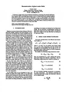
Figure 5.1

Plot depicting the function g(x). This plot was made with cs0 = 0.5,  = 0.1, f0 = 1, g0 = 0 and ϕ˙ 0 = 1. The exact behavior of g(x) is contrasted against the approximation (5.72). The behavior of g(x) is very linear except for small deviations for x < x0 . Note that at x0 (1 − c2s0 )8/55 ≈ 0.48 the plot of the exact behavior of g(x) stops abruptly as a result of the fact that g becomes non-real in this region. . . . . . . . . . . . . . . . . . . . . . . . . . . . . . . . . . . . . . . . .

98

5.2

Plot depicting the function f (ϕ) for different values of ω. This plot was made with cs0 = 0.5,  = 0.1, ϕ0 = 0, ϕ˙ 0 = 1.0, f0 = 1.0 and g0 = 0. We have also included a plot of the function f (ϕ) in (5.80) for comparison. . . . . . . . . . . . . . . . . . . 100

5.3

Plot depicting the regions of the ns -nt parameter space such that F diverges at the origin. The region in the upper left hand corner is the region of IR DBI inflation while the region at the bottom right hand corner corresponds to UV DBI. Only those values of ns and nt with ns < 2 and nt < 0 were considered, since any point outside that region would lead to an unphysical and/or non-inflationary action. . . 113

vi

ABSTRACT Non-Canonical Scalar Fields and Their Applications in Cosmology and Astrophysics by Christopher S. Gauthier

Chair: Professor Ratindranath Akhoury

In this thesis we will discuss several issues concerning cosmological applications of non-canonical scalar fields, which are generically referred to as k-essence. First, we consider two examples of k-essence. These are the rolling tachyon and static spherically symmetric solutions of non-canonical scalar fields in flat space. We find constraints on the form of the allowed interactions in the first case and on the choice of boundary conditions in the latter. For the rolling tachyon we find that at late times the tachyon matter behaves like a non-relativistic dust, thus making it a dark matter candidate. For the static spherically symmetric solutions we show that solutions which are finite at the origin must have negative energy density there. Next, we consider static spherically symmetric solutions of non-canonical scalar fields coupled to gravity as a way to explain dark matter halos as a coherent state of the scalar field. Consistent solutions are found with a smooth scalar profile which can describe observed rotation curves. The non-trivial solutions have negative energy density near the origin, though the total energy is positive. We also reconsider the no scalar hair theorems for black holes with emphasis on asymptotic boundary conditions and superluminal propagation. vii

After this we show that, for general scalar fields, stationary configurations are possible for shift symmetric theories only. This symmetry with respect to constant translations in field space should either be manifest in the original field variables or reveal itself after an appropriate field redefinition. In particular this result implies that neither k-essence nor quintessence can have exact steady state/Bondi accretion onto black holes. Finally, we find that stationary field configurations are necessarily linear in Killing time, provided that shift symmetry is realized in terms of these field variables. The next discussion outlines a general program for reconstructing the action of non-canonical single field inflation models from CMBR power spectrum data. This method assumes that an action depends on a set of undetermined functions, each of which is a function of either the inflaton field or its time derivative. The scalar, tensor and non-gaussianity of the curvature perturbation spectrum are used to derive a set of reconstruction equations whose solution set can specify up to three of the undetermined functions. This method is used to find the undetermined functions in various types of actions assuming power law type scalar and tensor spectra. Finally, we study a novel means of coupling neutrinos to a Lorentz violating kessence background. We first look into the effect k-essence has on the neutrino dispersion relation, and derive the neutrino velocity in a k-essence background. Next, we look at the effect on neutrino oscillations. It is found that if k-essence couples non-diagonally to the neutrino flavor eigenstates, this leads to an oscillation length that varies with the neutrino energy like λ ∼ E −1 . This is to be compared with the λ ∼ E dependence seen in mass-induced neutrino oscillations. While such a scenario is not favored experimentally, it places tight constraints on the possible interaction that a k-essence background can have with neutrinos.

viii

CHAPTER I

Introduction

The past two decades have been an exciting time for cosmologists and astrophysicists. This period has seen the beginning of true, precision cosmology. What was once a field that relied almost exclusively on qualitative predictions, was now able to test theories with definitive numerical accuracy. In this era we have seen two satellite missions: the Cosmic Background Explorer (COBE) and the Wilkinson Microwave Anisotropy Probe (WMAP), measure the spectrum of fluctuations in the comic microwave background radiation (CMBR). The first of these missions, COBE, confirmed that the CMBR has a black body spectrum [6], which was the final nail in the coffin for all competitors to the Big Bang Theory at that time. Both COBE and WMAP have also measured the minute temperature variations in the CMBR, leading to widespread support for cosmological inflation [7, 8]. During the period between COBE and WMAP, astrophysicists were able to measure the rate of the universe’s expansion. Two teams of astrophysicists [9] used type IA supernovae as “standard candles”, whose absolute brightness are remarkably consistent, and thus their distance away from us can be determined independently of their red-shift. This in turn allowed them to measure the rate of the expansion, which to the surprise of many, turned out to be increasing with time.

1

As exciting and important as these discoveries were for cosmology, they raised more questions than answers. Although COBE and WMAP confirmed many of the predictions of cosmological inflation, they could not tell us conclusively what mechanism was responsible for inflation. Similarly, while we have determined that the expansion rate of the universe has (at least recently) been accelerating, we still have no idea why it is accelerating. 1. Inflation Up until the early 1990’s, the status of the Big Bang model was still in doubt. Although it was the favored model by that time, there were still problems with the theory that gave some physicists reason to object. In particular, there were three outstanding problems with the Big Bang. The first of these was called the horizon problem. In the classical model of the Big Bang, the comoving causal horizon at −1/2 −1

the time of photon decoupling was approximately 180Ω0

h

Mpc. However, the

present comoving horizon of the universe is considerably larger; 5820h−1 Mpc1 . This means that our observable universe today consists of approximately 105 regions that were causally disconnected from each other at the time when the CMBR settled into its present state. However, despite this, the CMBR is remarkably smooth across the entire sky. Such homogeneity over causally disconnected regions is something the classical Big Bang can not explain satisfactorily. The second problem for the classical Big Bang model is the flatness of the universe’s geometry. If one does a simple study of the Friedmann equations, they would quickly raise the issue that a flat universe is not a stable solution. If we write the 1 This

assumes that the universe is flat

2

Friedmann equations in terms of the density parameter Ω what we find is that K

(1.1)

a2 H 2

where Ω =

ρ 2 2 H2 , 3Mpl

and H =

a˙ a

= Ω − 1,

is the Hubble parameter. Here, K is a constant

that represents the intrinsic spatial curvature of the universe, and the scale factor a can always be defined such that K = 0, ±1. If K vanishes then it follows that the density parameter Ω is a constant and equal to the critical density Ω = 1. When this happens the universe has a flat, Euclidean spatial geometry. On the other hand, if K is nonzero then Ω is not at the critical value. If the expansion of the universe is decelerating, then the factor a2 H 2 = a˙ 2 is getting smaller, which means that the deviation of Ω from the critical density will continue to get larger as time goes on. This was a troubling notion for supporters of the Big Bang at that time because all evidence seemed to indicate that we live in an extremely flat universe. Current estimates place the present day value of |Ω − 1| at less than 0.01. This means that our universe is so flat that in order to end up within the presently observed range of Ω, then at the time of the Planck era the deviation of Ω from the critical density would have to be smaller than one part in 1060 . Finally, the third big problem with the Big Bang is the paradoxically low density (if not the absence) of monopoles. If our theory of gauge fields is correct, which all Earth based experiments suggest, then a copious number of monopoles should have been produced at the beginning of the Big Bang [10]. This absence (so far) of monopoles in the universe is another puzzle that the classical Big Bang is unable to account for. As luck would have it, Alan Guth suggested a simple solution to these problems [11], a solution that would later be known as cosmological inflation (or simply in2M 2 pl

2 = denotes the reduced Planck mass: Mpl

3 . 8πG

3

flation). Guth’s model involved giving the universe a short period of accelerated expansion. This rapid expansion is powered by a positive vacuum energy density that is sourced by a scalar field, called the inflaton, that lies in a metastable vacuum. Since this state is unstable due to quantum fluctuations, the inflaton will eventually tunnel out of the metastable vacuum and into a stable one, creating bubbles of true vacuum in the bulk of false vacuum. If these bubbles are produced at a large enough rate, they will collide with one another, releasing the energy stored in the walls of the bubbles as radiation, thereby reheating the universe and ending inflation. Guth’s initial motivation for this idea was to solve the monopole problem. In the inflationary universe, monopoles created just before the inflationary expansion are diluted away by the rapidly increasing volume of our observable universe. Guth’s model, however, turned out to solve more than just this problem. As it turns out an initial rapid expansion also solved the horizon and flatness problems. In regards to the horizon problem, inflation reconciled this paradox by allowing for the observable universe to occupy a casual patch before inflation started, during which the universe could achieve thermal equilibrium. Inflation also gave an explanation for the flatness problem since during an accelerated expansion a˙ is getting larger, and thus as (1.1) implies, Ω will be driven towards the critical density. Unfortunately, Guth’s original inflation model had a serious problem that made it unworkable; a fact he acknowledged when he first introduced his model. In Guth’s model of inflation, the decay rate of the metastable vacuum has to be small enough to provided for a sufficient amount of inflation, but has to be large enough for the bubbles of true vacuum to be produced at a fast enough rate for them to collide and reheat the universe. These requirements were found to be incompatible, leaving Guth’s model dead on arrival. However, the idea that an early exponential expansion

4

could solve three of the biggest objections to the Big Bang was too tantalizing to give up. Fortunately, soon after Guth published his findings, Andrei Linde [12] and independently Andreas Albrecht and Paul Steinhardt [13], came up with a new model of inflation that was soon called slow roll inflation. In this realization of inflation the inflaton is a scalar field with a potential that has a zero energy vacuum state. When the inflaton is displaced from the vacuum, the inflaton potential will be nonzero, providing the vacuum energy needed to drive inflation. When the inflaton reaches the vacuum, inflation ends and the energy in the inflaton field is converted into radiation that reheats the universe. Today most models of inflation are based on the paradigm set by Albrecht and Steinhardt, and Linde . If all inflation did was explain away problems with the Big Bang, then inflation would be regarded by critics of the Big Bang as nothing more than an ad hoc fix. However, as it turns out inflation makes a testable prediction. Due to quantum fluctuations in the behavior of the inflaton, the value of the vacuum energy density will vary at different points in space. Through a careful analysis [14] it was shown that this variation, although slight, would eventually leave its mark as spatial fluctuations in the CMBR. Specifically, nearly all inflation models make the generic prediction that at large distance scales the magnitude of the fluctuations in the CMBR temperature, should be relatively independent of the size of the region of the fluctuation. The possibility of confirming this prediction was one of the reasons that the COBE satellite was created. COBE’s observation of nearly scale invariant temperature fluctuations solidified the support for cosmic inflation and put to rest any serious doubts about the Big Bang.

5

2. Dark Energy After Edwin Hubble made his landmark observation that the universe was expanding, many physicists assumed that due to the universal gravitational attraction of matter, this expansion rate should be getting smaller as time goes on. However, in 1998 this view was quickly thrown out of the window [9]. As it turns out not only is the expansion of the universe not decreasing, but it is actually accelerating. At present, the best answer we can give for this accelerating expansion rate is the existence of a positive vacuum energy density pervading the universe. This vacuum energy can be modeled in general relativity as a cosmological constant term. The cosmological constant (c.c.) was originally proposed by Einstein as a means to create a model of a static universe. After Einstein heard about Hubble’s discovery, he recanted his belief in a static universe, and declared his inclusion of the c.c. “his biggest blunder”. However, with these recent insights it seems that Einstein’s blunder may not have been a blunder after all. Although the accelerated expansion can be modeled by the inclusion of a c.c., this does not explain why a c.c. exists. For particle physicists, the question was not so much why there is a c.c., but why is it so small? In the calculation of loop corrections to the effective action of the standard model, the correction to the c.c. term Λ is of the order of the Planck scale Λ ∼ Mpl4 ∼ 10109 eV4 . This is staggeringly higher than the currently estimated value of the c.c, which is Λ ∼ 10−11 eV4 ; off from the expected value by a factor of 10120 ! This gigantic discrepancy has been dubbed the “the worst prediction in physics”. While the value of the corrections to the c.c. can be eliminated by counter terms during renormalization, it is troubling that such large numbers must be contrived in such a way as to result in a number that is smaller by a factor of 10−120 of the

6

original numbers. Unfortunately, there has been little success in trying to explain the nature of dark energy. Some of the ideas that have been proposed include: quintessence [15, 16], anthropic selection [17], extremely large cosmic voids [18]. One proposed explanation, which uses a scalar field with a non-canonical action as the source of the c.c., is called k-essence [19, 20, 21]. This model has several novel features and will be a primary focus of this thesis. 3. K-essence and K-inflation Dynamical scalar fields have held a special place in modern physics. When physicists encounter new phenomena, often times a phenomenological model based on scalar fields is used in order to gain some initial understanding. Examples of these include: the Yukawa model of the strong force [22], the Landau-Ginzburg model of superconductivity [23], the Higgs model [24], the axion [25], and most recently cosmological inflation [11, 12, 13]. Scalar fields enjoy the advantage of having the simplest behavior under general space-time coordinate reparametrizations, making them natural tools for building toys models. The action of a real relativistic scalar field φ, in a general N -dimensional space-time background is given by Z (1.2)

Sscalar =

√

 1 µν d x −g g ∂µ φ∂ν φ − V (φ) , 2 N



where gµν is the background space-time metric, g = det(gµν ), and V (φ) is the potential energy function of φ. Of all field theory actions, this is by far the simplest. In addition to their simplicity, scalar fields also have the unique and useful property of being able to have a constant nonzero vacuum expectation value (i.e., hφi 6= 0) while still maintaining Lorentz invariance. This property is a prized feature of scalar fields, and it is the reason that models like the Higgs mechanism and inflation are 7

possible. Although (1.2) is the most widely used theory of scalar fields, it would break no known fundamental physical principles if more general scalar field actions were considered, such as Z S=

√ dN x −gL(X, φ),

where X = 21 g µν ∂µ φ∂ν φ. Here the function L is the Lagrangian of the scalar field and can be almost any function of two variables. While there are no theoretical objections to such general scalar field actions, many physicists paid little attention to such possibilities, as there didn’t seem to be any good reason to consider them. Since there are an infinite number of possible functions L to consider, without some motivation from theory or experiment, little can be done in the way of studying them. Recently, however, this class of theories has started to attract attention due to new discoveries in both theory and experiment. On the theory side, advances in our understanding of string theory have led to a deeper appreciation of the importance of D-branes [26]. The effective action of the D-brane degrees of freedom can be cast into the form of the Dirac-Born-Infeld (DBI) action, an action that was previously proposed as an alternative to the standard electrodynamical action. The simplest DBI action describes the motion of a D3-brane along a single direction: Z SDBI = −

i p √ h d4 x −g f −1 (φ) 1 − 2f (φ)X − f −1 (φ) + V (φ) .

The features of this action will be discussed in depth in chapter §V. For now we should note that this is an example of a non-canonical scalar field action, and has found possible applications in cosmology [27, 28].

8

In the realm of phenomenology, some have considered the possibility of using non-canonical scalars to explain the coincidence problem [15, 29]. Put simply, the coincidence problem refers to the fact that the dark energy, which is now the main driver of cosmic expansion, has only recently been the dominant component of the total energy density of the universe. If this were not true, and dark energy had become dominant earlier on, it is inconceivable that matter would be able to form clusters large enough to create galaxies. In order to get galaxies there must have been a period of matter domination, between the periods of radiation and dark energy domination. Attempts have been made to explain this coincidence as a consequence of the behavior of dark energy. These proposals have concentrated on models that exhibit the so called tracker solution. In these kinds of models, a scalar field is the source of the dark energy, and its action is setup so that the equation of state of the scalar field only starts to behave like vacuum energy after matter has come to dominate over radiation. One model that has tracking solutions is quintessence [15, 16]. Quintessence uses a canonical scalar field with a suitably chosen potential to get the correct tracking solution needed to solve the coincidence problem. While it is possible to solve the coincidence problem with quintessence, it was quickly realized that to do so requires an incredibly high level of fine tuning; defeating the entire purpose behind quintessence in first place. An alternative to quintessence, dubbed k-essence (the “k” standing for kinetic), works the same way, but uses non-canonical scalar fields as the source of the vacuum energy [19, 20, 21]. The advantage k-essence has over quintessence is that tracker solutions are the general solutions of k-essence. Thus, k-essence does not require the high level of fine tuning that quintessence does if one wishes to solve the coincidence

9

problem. However, the naturalness of k-essence does come at a price. It was discovered [30] that any k-essence model created to solve the coincidence problem would have a brief period when fluctuations in the k-essence field propagate at superluminal speeds. At first this may seem like a deal breaker for k-essence; however, it was later shown by the authors in [31] that despite the superluminal speeds, causality is preserved in k-essence. An interesting feature of k-essence is that, unlike quintessence, the kinetic energy of k-essence can source the cosmological constant. Vacuum energy has the critical property that it is constant with respect to the scale factor a of the universe. The kinetic energy of a canonical scalar field leads to an energy density that goes like ∝ a−6 , which means that it dissipates too quickly, even more quickly than matter (∝ a−3 ) and radiation (∝ a−4 ). However, because of the non-trivial dependence of the k-essence Lagrangian on X, it is possible to get a vacuum energy entirely through the kinetic energy. Therefore, it is possible to have so called “kinetic” k-essence theories; actions that only depend on X. This ability to create vacuum energy has also made k-essence a possible candidate for the inflaton. Theories that attempt to explain inflation in the context of k-essence have been dubbed k-inflation [32]. K-inflation models have a number of interesting features that set them apart from the typical slow roll inflation models. One such feature of k-inflation is that fluctuations in the inflaton field can propagate at speeds different than the speed of light. When viewed as a continuous classical medium, the speed of fluctuations cs in a general scalar field is (1.3)

c2s =

∂p/∂X LX = . ∂ρ/∂X LX + 2XLXX

Here p and ρ denote the pressure and energy density of the scalar field. The speed cs is typically referred to as the sound speed. Clearly, from (1.3) we can see that 10

cs will be equal to one for a canonical scalar field3 . However, for k-essence cs will in general be different from, and can even exceed, the speed of light [31, 33]. This can lead to some interesting consequences in the case of k-inflation models since the spectrum of primordial curvature perturbations depends on the sound speed of the k-essence perturbations [34]. Finally, another reason k-inflation has been under consideration is because they often predict large non-gaussianities [35, 36]. In canonical inflation models, nongaussianities can only be produced through interactions that are cubic or higher order in the inflaton field variable, or indirectly through the inflaton’s interaction with gravity. However, the non-gaussianity produced in these ways is on the same order as the slow roll parameters [37, 38], and is therefore small. Non-gaussianities in k-inflation on the other hand can be quite substantial due to the possible nonlinear dependence of the action on X. Thus, non-gaussianities are an important discriminator between canonical and non-canonical inflation models. The application of non-gaussianities to finding the form of the k-inflation action is discussed in chapter §V of this thesis. Therefore, non-canonical scalars have the ability to explain the late-time accelerated expansion of the universe, and the related coincidence problem through kessence; and they can also provide an alternative explanation for the primordial accelerated expansion of the universe through k-inflation. 4. Dark Matter The idea that the universe contains particles that we have yet to observe is an old idea in physics. Several times when physicists were faced with an unexpected observation or a difficultly with theoretical models, a new, as yet unseen particle 3 Throughout

this thesis we will take the natural units so that c = 1.

11

turned out to be the solution. This has happened in the case of the neutrino [39], the π meson [22], and the charm quark [40]. In light of this trend, it’s no surprise that when galactic rotation curves were found to be in conflict with the naive expectation of Newtonian mechanics [41], physicists immediately began to propose all kinds of new particles to explain the discrepancy. According to the results from the surveys of galactic rotation curves, the distribution of observable matter in all galaxies studied so far indicate that there is not enough observable matter on the edges of these galaxies to explain the high rotational velocity there. In light of these observations, it is reasonable to suggest that there is additional matter that, although invisible to our telescopes, nevertheless comprises the majority of the mass content of galaxies, and by extension our universe. The history of dark matter (so named because it is required by definition to be decoupled from electromagnetic interactions) has a long history in astrophysics, and yet in all this time, its true nature has so far eluded our understanding. At first it was suggested that dark matter may have a much more mundane original; perhaps composed of the remnants of stars, or the puny sized gas giants that weren’t able to become stars. For a time, neutrinos were considered a possible candidate for dark matter [42]. However, as we have learned more about the required properties of dark matter, it has become apparent that these run of mill solutions are not enough to explain the observations. Clearly more unconventional options have to be considered. Many of the current explanations for dark matter rely on the existence of some exotic, as yet unseen, particle. The proposed identity of the dark matter candidate has been primarily motivated by theories that go beyond the standard model, such as supersymmetry [43]. Computer simulations of structure formation in the early universe have also helped in determining the required properties of dark

12

matter. As popular as this approach is among physicists, there are other, albeit more radical alternatives to dark matter. One of these is Modified Newtonian Dynamics (MOND), which attempts to explain the observed discrepancies as a modification of gravity at weak gravitational fields [44]. These models, however, have met with limited success. Another proposal for explaining dark matter, that we will be studying in chapters §II-IV, is the idea that dark matter is really a k-essence condensate. In these chapters we will discuss the conditions needed to have stable k-essence halos around galaxies. 5. Neutrino Oscillations If there is a k-essence field pervading the universe, then it is natural to ask what effects it might have on the standard model family of particles. From the perspective of effective field theory, it is almost a given that if a k-essence background exists, it will directly couple to all other matter that is present. Due to its importance in cosmology and astrophysics, the neutrino presents the most interesting case in which to study possible k-essence/matter interactions. In 1930 Wolfgang Pauli [39] proposed the existence of a (at that time undetected) particle, later called the neutrino, that was responsible for carrying away the energy and momentum that was missing in the decay products of beta decay. Observations of the energy spectra of the beta decay products led to the initial conclusion that the neutrino was massless. However, the notion that neutrinos may have a small but nonzero mass has been a persistent idea in modern particle physics. For some time the data did not imply any need for a nonzero neutrino mass, until neutrino observatories measured a deficit in the expected number of neutrinos being produced

13

by our sun [45]. Even before this anomaly was found physicists had considered the possibility of mass causing just this kind of result [46]. In order to understand how neutrino mass can explain the solar neutrino problem we first have to note that neutrinos come in three different varieties: the electron neutrino, the muon neutrino, and the tau neutrino. Early solar neutrino detectors were only sensitive to the electron neutrino species, since this is the only neutrino flavor that is produced in the kinds of reactions that take place in the sun. It was found that if the various neutrino flavors have different masses, then this can lead to the phenomenon of neutrino oscillations. This means that if a neutrino of the electron variety is created at the source (in this case the sun) then as it travels to an Earth based detector, the probability of observing this neutrino in the electron neutrino state will oscillate with respect to the distance traveled. A simplified analysis of neutrino oscillations when there are N different flavors, shows that the probability of observing an f 0 flavored neutrino some distance L away from the source of the neutrino where it was f flavored is P (νf → νf 0 ) = δf f 0 − 4

X

Re(Uf∗i Uf 0 i Uf j Uf∗0 j ) sin2



i>j

(1.4)

+2

X

Im(Uf∗i Uf 0 i Uf j Uf∗0 j ) sin

i>j



∆m2ij L 2E

∆m2ij L 4E



 .

Here, E is the energy of the neutrino and ∆m2ij = m2i − m2j , where the mi ’s are the masses of the neutrino mass eigenstates. The indices i and j enumerate the neutrino mass eigenstates and assume the values i, j ∈ {1, 2, ..., N }. Here the Uf i ’s are the matrix elements of the so called neutrino mass mixing matrix. Essentially, the matrix U is an SU (N )4 matrix that transforms the neutrino mass eigenstates into the neutrino flavor eigenstates. As long as U is non-diagonal, then the last two 4 This assumes that the neutrinos are Dirac fermions. If they are Majorana fermions then the mixing matrix must be an U (N ) matrix.

14

terms of (1.4) will be nonzero and neutrinos will undergo flavor oscillations. Thus, even if only electron neutrinos are being produced in the sun, as long as there is a mass difference between the neutrino mass eigenstates, some of those electron neutrinos will “flip” into mu or tau neutrinos when they arrive on Earth. Since the early neutrino observatories could not detect the mu and tau neutrinos, those electron neutrinos that flipped could not be detected. Therefore, the solar neutrino flux would have been lower than expected [47]. Today, these “lost” neutrinos have been detected, and are enough to account for the missing solar neutrino flux [48], confirming that neutrinos do indeed undergo flavor oscillations. This has been widely interpreted as evidence that neutrinos have mass5 . However, other mechanisms that can also induce neutrino oscillations [49, 50, 51, 52, 53] are often ignored. Thus, it is not a given that neutrino oscillations confirm the existence of neutrino masses. The critical feature needed to induce neutrino oscillations is a spatially varying phase difference between the energy eigenstates of the neutrino. Although mass can create this phase difference, there are many other ways in which to create flavor oscillations. Any coupling term in the neutrino Lagrangian that is non-diagonal in the neutrino flavor space is capable of inducing neutrino oscillations. In chapter §VI, we will study the possibility of k-essence induced neutrino oscillations (KINO) [5]. In this new mechanism, the neutrinos couple to k-essence by replacing the spacetime metric in the neutrino action with a k-essence induced metric. In addition to modifying the dispersion relation of the neutrinos, we will show that if this coupling is non-diagonal in the neutrino flavor basis, neutrino oscillations occur even in the absence of neutrino masses. 5 To be more accurate, observation of the missing neutrino flux is evidence that the neutrino mass eigenstates have different masses. It is still possible for at least one of the neutrinos to be massless.

15

5. Outline of Thesis This thesis is organized as follows. Chapters §II and §III discuss the possibility of dark matter halos as k-essence condensates. In chapter §II we investigate k-essence halos in flat space and in the FRW metric. In particular, we study the specific cases of the rolling tachyon, and static spherically symmetric solutions of general k-essence Lagrangians. In chapter §III we extend the analysis of static spherically symmetric solutions in chapter §II to include the effects of gravitational back-reaction. Chapter §IV is an outgrowth of the work done in the previous two chapters, and here the question of when stationary solutions are possible in k-essence is addressed. The existence of stationary k-essence solutions is addressed in the context of black hole accretion, where one typically uses such solutions in order to simplify the analysis. In chapter §V we change the subject from k-essence to k-inflation, and discuss a procedure for reconstructing the k-inflation action from cosmological observables. Next, in chapter §VI we explore the possibility of k-essence/neutrino interactions. In that chapter we will study the effects that a hypothetical k-essence/neutrino coupling has on the motion and flavor oscillations of neutrinos. Finally, in chapter §VII we review our major findings in the conclusion.

16

CHAPTER II

Classical Solutions of K-essence Theories

2.1

Introduction

Scalar field theories with higher derivatives play an essential role in the effective field theory approach (for reviews see [54]). An example is provided by the chiral Lagrangian which provides a good description of the strong dynamics at low energies. Applications of higher derivative theories to cosmology have also become popular in the last few years: examples here are effective field theories of the rolling tachyon [55, 56], DBI inflation [27, 28, 57], and k-essence [19], which attempts to provide a dynamical explanation of the so called coincidence problem and the accelerated expansion of the universe. Recently [35], such higher derivative actions have been shown to enhance the non-gaussian fluctuations in the cosmic microwave background. Theories with higher derivatives have the possibility of modifying the dispersion relations and hence may potentially lead to superluminal propagation. This aspect has been studied in detail in [58] where it was shown that causality and the absence of superluminal propagation require certain coefficients of the effective Lagrangian to be positive definite, which in turn has consequences for phenomenology [58, 59]. Thus, the constraints of causality and hyperbolicity of the equations of motion play a particularly important role in such theories. Another recent striking example is

17

the no-go theorem proved in [30]. It was shown there that in the context of the original k-essence theories [19], it is impossible to simultaneously resolve the coincidence problem and the accelerated expansion of the universe without encountering problems with superluminal propagation. In this chapter we apply the constraints [60, 61, 62, 63] that the equation of motion of the scalar field has a well defined initial value problem and there is no superluminal propagation of the small fluctuations around classical solutions in higher derivative theories. In particular we discuss in sections §2.3 and §2.4, respectively, the case of the rolling tachyon and the static solutions to the equations of motion of a general scalar theory with higher derivatives. For the case of the tachyon we consider a general Lagrangian of the form L = V (φ)K(X), with V the potential of the tachyon and X = 21 g µν ∂µ φ∂ν φ, and find the constraints on K(X) and the potential such that the the energy density is finite but the equation of state parameter goes to zero at late times up to small corrections. We find that in order achieve this it is not necessary for K(X) to vanish as φ˙ → 1, but only that it be bounded. Other constraints on K are obtained which allows for a more general framework for the rolling tachyon than was previously considered. The only constraint on the potential is that a3 V → 0 at late times, where a is the scale factor. The physical motivation is that the tachyon could then be considered as a possible candidate for dark matter [64]. In section §2.4 we discuss the static spherically symmetric solutions to the equations of motion for the most general scalar field Lagrangian with higher derivatives in flat space which are consistent with hyperbolicity and causality. We find the interesting result that for scalar field solutions that are finite at the origin, causality requires its first derivative to vanish there. Furthermore, even though the total energy is positive, the energy density for such solutions is negative at the origin. A physical motivation for

18

this study arises from the possibility that such scalar fields could describe the dark matter halos around galaxies [63]. In section §2.2 we set up the problem and review some results concerning the criteria for superluminal propagation and hyperbolicity of the scalar field equations. In the concluding section we discuss the results. 2.2

Preliminaries

In this chapter we will be interested in scalar field theories with a Lagrangian of the general form L = L(X, φ). Here, X = 21 ∂ µ φ∂µ φ. The equations of motion for the scalar field are given by (2.1)

˜ µν ∇µ ∇ν φ = Lφ − 2XLXφ , G

˜ µν = LX η µν + LXX ∂ µ φ∂ ν φ. where G

Throughout this chapter we will be using the notation LX =

∂L , ∂X

Lφ =

∂L ∂φ

and so on. In (2.1), Gµν plays the role of an effective metric in which the scalar field propagates. For an equation of this type to have a well defined initial value (or Cauchy) problem and to satisfy global hyperbolicity, the following conditions must hold1 [60, 61, 62] LX > 0,

LX + 2XLXX > 0.

If u = 0 is the characteristic surface and nµ = ∂ µ u, then the speed of propagation of the small disturbances is given by solving LX n2 + LXX (nµ ∂µ φ)2 = 0. From this, one deduces the maximum speed to be   r   ~ ~ 2 W0 ~n|~·nW| + 1 + W02 − ~n|~·nW| 0 n = , |~n| 1 + W02 1 See

appendix §A for further discussion of the Cauchy problem and causality in k-essence

19

where, Wµ =

q

LXX ∂ φ. LX µ

The two cases discussed in this chapter are the time-like

spatially homogenous and static spherically symmetric ones. The expressions for the propagation speeds in the two cases are respectively, r n0 LX φ˙ 2 = , X= |~n| LX + 2XLXX 2 r 0 φ02 LX + 2XLXX n = , X=− . |~n| LX 2 Here, a dot denotes differentiation with respect to t, and a prime denotes differentiation with respect to r. From these it is easy to see that there is superluminal propagation when LXX < 0. In summary, the conditions of hyperbolicity and no superluminal propagation may be stated as (2.2)

LX > 0,

LX + 2XLXX > 0,

LXX ≥ 0.

For future reference we note that in the static spherically symmetric case when there is no superluminal propagation, r (2.3)

LX ≥ 1. LX + 2XLXX

When gravity is included, the effective scalar metric now becomes (2.4)

Gµν = LX g µν + LXX ∂ µ φ∂ ν φ.

We require this metric to be Lorentzian. In particular in order to have a consistent definition of temporal and spatial directions the largest eigenvalue of (2.4) must be positive while the other three must be negative. This can be shown to be true [61, 62] only if the first two conditions in (2.2) are satisfied (with X = 21 g µν ∂µ φ∂ν φ now) while the last one once again avoids [58, 60] superluminal propagation.

20

2.3

The Rolling Tachyon

Sen [55] has discussed the qualitative dynamics of a tachyon field in the background of an unstable D-brane system and conjectured that the simplest description within an effective field theory framework can be provided by the following Lagrangian: L = V (φ)K(X), with φ the scalar field, and q K(X) = − 1 − φ˙ 2 ,

(2.5)

V (φ) = V0 exp(−φ).

The cosmology of this model in the FRW background has been studied in [55, 56, 64], and a particularly surprising result is the existence of solutions with exponentially vanishing pressure at late times, but a nonzero energy density. Since there is no compelling reason for the precise forms in equation (2.5), in this section we keep K and V arbitrary (apart from the mild assumptions below) and determine from the constraints (2.2), the conditions under which the equation of state for tachyonic matter becomes ω = 0 at late times up to small corrections. The tachyon could then be considered a dark matter candidate in a wider class of models than originally envisioned. Consistent with the fact that we are dealing with the case of a rolling tachyon, we will make the following assumptions about the potential V and the kinetic term K: first is that K ≤ 0; second, the range of φ˙ is bounded; third, K is bounded as φ˙ → 12 ; and fourth, the potential V (φ) is positive, has a maximum at φ = 0 and monotonically decreases to zero at φ = ∞ where it is a minimum. The equations of motion for the scalar field and the scale factor a(t) are3 ∂ρt

φ¨ = −3H 2 We 3 We

LX ∂φ φ˙ − , LX + 2XLXX LX + 2XLXX

will take the upper limit of φ˙ to be 1 in the appropriate units. work in units where 8πG =1 3

21

H 2 = ρ = ρt + ρm .

For the homogenous FRW background 2X = φ˙ 2 > 0. ρt = 2XLX − L is the tachyon energy density and ρm is that of the rest of matter and ρ is the total energy density. H=

a˙ a

is the Hubble factor. Note that from the first inequality in equation (2.2) and

L < 0, it is easy to see that ρt > 0. Thus, the non-vanishing of the energy density at all times including late times is strictly a consequence of LX > 0. The equation of state parameter for the tachyon is, ωt =

(2.6)

L K = . 2XLX − L 2XKX − K

Using the φ field equation of motion it is straightforward to show that (2.7)

ρ˙ t =

d (2XLX − L) = −6HXLX = −3H(1 + ωt )ρt . dt

The inequality in equation (2.2) then implies that the tachyon energy density is a monotonically decreasing function of time and ωt > −1. The Hubble factor itself is monotonically decreasing in time as can be seen from 3 H˙ = − ((1 + ωm )ρm + (1 + ωt )ρt ) , 2 Defining y =

√

2X, and using the factorized form for the tachyon Lagrangian, the

tachyon equation of motion may be written as, (2.8)

dy yKy − K =− dt Kyy

 ∂V ! Ky ∂φ 3H + . yKy − K V 

The constraints given in equation (2.2) for the initial value problem to be well defined and the absence of superluminal propagation are expressed in terms of the new variable as: (2.9)

Ky > 0,

Kyy > 0,

Kyy >

Ky . y

Note that whenever V → 0, then Ky → ∞ such that LX > 0. As we will see below, it is this simple fact that guarantees that the tachyon energy density is nonzero and 22

positive in the limit t → ∞, while ωt vanishes; indicating that the tachyon field acts like a non-relativistic dust at late times. Let us consider equation (2.8) at late times. We first discuss the conditions on the potential under which the second term in the brackets is dominant. Let us define the term inside the square brackets in this equation as g, then dg −KKyy = . dy (yKy − K)2 Since K < 0, we see from (2.9) that

dg dy

> 0. The maximum value of g is thus at

y = 1, which is gmax ≤ 1. Moreover, H is monotonically decreasing. Let us now write for late times φ = t + θ(t), with θ(t)  t. It is easy to check from the above results that the second term inside the brackets in equation (2.8) dominates over the first for late times as long as V → 0 faster than

1 a3

when t → ∞. This condition

on the potential will reappear below. Since the overall factor outside the brackets in (2.8) is negative, and since

∂V ∂φ

< 0 from our assumptions, the above discussion shows

that y is monotonically increasing as it goes to 1 at late times. In addition, since y is bounded at y = 1, then y˙ = 0 at y = 1. Therefore we conclude that as y → 1, (2.10)

Ky = 0, Kyy

K = 0. Kyy

As mentioned earlier, Ky → ∞ for late times while K is bounded. Thus, the second of the above conditions is not a new requirement since the first implies that as y → 1, Kyy > Ky . It should be noted that the condition for the absence of superluminal propagation only implies that Ky < y, Kyy Thus the condition (2.10) is much stronger.

23

Let us now expand equation (2.8) about the point y = 1 by writing, φ = t + θ(t) with θ˙ < 0 and θ  t. Using (2.10), it is straightforward to get, " # ∂V ∂φ ˙ 3H + θ¨ = −θλ , V   Kyyy Ky λ= 1− (2.11) (y = 1). 2 Kyy Integrating this we get (taking φ˙ ≈ 1 to leading order) θ˙ = −αa−3λ V −λ , where α is a constant. Consistency with the boundary conditions require λ < 0. Since θ  t, we see that with a negative λ, θ˙ vanishes like a3 V → 0 as t → ∞, which is exactly the condition derived earlier for the term involving the potential V to dominate over the first one in equation (2.8). Thus, λ < 0, or equivalently, Kyyy > Kyy at y = 1, which is a new constraint on the allowed forms of K. We are now in a position to prove that the equation of state parameter vanishes at y = 1 up to small corrections. From equation (2.6) we can obtain, yKy2 − KKy − yKKyy dωt = . dy (yKy − K)2 Since K ≤ 0, and Ky and Kyy are both positive, we see that ωt is a monotonically increasing function of y. Its maximum is therefore at y = 1. Near y = 1 we can write ωt ≈

˙ y (1) K(1) + θK . Ky (1)

However, we have argued above that Ky (1) is infinite, thus ωt = 0 apart from corrections which vanish like a3 V at late times. 2.4

Background Static Solutions Consistent With Causality

We next consider the static spherically symmetric solutions to the equations of motion of the scalar field in flat space-time. The equation of motion for a static 24

scalar field φ(r) is (2.12)

2 φ + r 00



LX LX + 2XLXX



φ0 +

Lφ − 2XLXφ = 0. LX + 2XLXX

02

In the above, X = − φ2 . From section §2.2, the combined constraints of hyperbolicity and absence of superluminal propagation now give the following bound for the coefficient of the φ0 term for all r (see equation (2.3)): (2.13)

δ=

LX ≥ 1. LX + 2XLXX

Here we consider only solutions to (2.12) which are finite at the origin. We first want to determine the appropriate boundary condition for φ0 at r = 0. We will use a series expansion method for φ near r = 0 to guide us to the correct choice. Even though the coefficient δ is not a constant but dependent on φ, we know that independent of r, δ ≥ 1. Therefore, since we are interested in finding the indicial equation in order to determine the boundary condition for φ0 , we may treat δ as a constant. The same applies for the last term in (2.12) as long as we restrict ourselves to solutions which are finite at the origin. These two complications do not affect the indicial equation. With this in mind, let us look for a series solution of the form (2.14)

φ = rs (c0 + c1 r + c2 r2 + c3 r3 + · · · ).

From this we get the indicial equation, s(s − 1 + 2δ) = 0. Since δ ≥ 1 for all r, we see from (2.14) that in order for φ to be finite at the origin only the solution with s = 0 is allowed. Substituting this expansion into (2.12) we see by matching equal powers of r that c1 = 0. Thus, the boundary condition for this problem that is consistent with (2.13), and the finiteness of φ at the origin is φ0 = 0 at r = 0. We now consider the analog of equation (2.7). Let us define γ = −2XLX + L. Then

25

using the equation of motion we obtain 2 dγ = − φ02 LX . dr r

(2.15)

Since LX > 0, we see that γ is a monotonically decreasing function of r. Therefore, the minimum of γ is at infinity. As r → ∞, the solutions to the equations of motion 1 r3

must be such that γ → 0 faster than

in order to keep the total energy content

finite. This implies that γ > 0 as r → 0. From the boundary condition on φ0 at r = 0, we see that γ = L > 0. On the other hand, in the static limit the Hamiltonian density H becomes H = −L. Thus, we conclude that at r = 0, the energy density H is negative. It is easy to see that the total energy in the static limit is, however, always positive: Z E = −4π

Z

2

r Ldr = −4π

(γ − φ02 LX )r2 dr.

Consider the integral over γ. Integrating by parts and using the fact that γ vanishes faster than

1 r3

as r approaches infinity, we get Z

1 γr dr = − 3 2

Z

dγ 3 2 r dr = dr 3

Z

φ02 LX r2 dr,

where the last equality follows from (2.15). Combining everything, we find that 4π E= 3

Z

φ02 LX r2 dr,

which is manifestly positive definite. When such a theory is coupled to the Schwarzschild metric, we can look for solutions to the combined equations for both gravity and scalar matter. Such a situation could be relevant for understanding the formation of dark matter halos around galaxies [63]. Though the above analysis has been performed in flat spacetime, our considerations indicate that at least solutions of the scalar field equations 26

that are finite at the origin should not be relevant to such a scenario if one takes the view that negative energy densities are not allowed. The detailed question of the solutions of the scalar field in the presence of gravity is the subject of the next chapter. Nevertheless, it is interesting that the model we have considered in this section has solutions which violate the weak energy condition at the origin. 2.5

Conclusion

Using the requirement that the field equations are always hyperbolic (and hence the Cauchy problem is well defined) we have obtained a set of consequences for two different problems of physical interest. For the case of the rolling tachyon in a homogenous FRW background, we have obtained constraints on the forms of the potential and the kinetic terms such that the equation of state of the tachyon vanishes at late times up to small corrections. The tachyon could then be considered a dark matter candidate. The key observation here was that what is required for this to happen is that K remains bounded but not necessarily zero at late times, while Ky goes to infinity. The latter in fact guarantees that the energy is non-vanishing in this limit. Other requirements are given by equations (2.10), the potential V is such that a3 V → 0 at late times, and that λ defined in (2.11) be negative. It is easy to check that the choice (2.5) does in fact satisfy all the requirements, but is not unique. The class of models is thus larger than the original. We have also looked quite generally at the problem of the static spherically symmetric solutions to the equations of motion of the scalar field described by the Lagrangian of section §2.2 and found that if we require the finiteness of the scalar field at the origin, then the solutions consistent with causality have the property that the

27

energy density becomes negative at the origin. This example brings out very clearly the role that causality plays in the choice of boundary conditions. There have been attempts in the literature [63] to use such scalar field models to describe dark matter halos around galaxies. Clearly, solutions which are finite at the origin will not do the job. However, it is interesting to speculate if this negative energy density at the origin is indicative of an attractive force, analogous to the Casimir effect (but of course classical), at the center of galaxies.

28

CHAPTER III

K-essence Galactic Halos

3.1

Introduction

Recently there has been a lot of interest in the applications of non-canonical scalar field theories in cosmology. This is due mainly to the fact that the energy-momentum tensor in such field theories has the potential to describe cosmological fluids with negative pressure, which is a necessary ingredient for accelerated expansion. Examples are: k-essence [19], which attempts to explain the accelerated expansion of the universe as well as the coincidence problem, the DBI action [27, 28, 57, 35], tachyonic matter [55, 56, 1], the ghost condensate model [65] and the Chaplygin gas model [66]. They are also interesting in the context of inflationary models [32, 3]. Since these theories contain non-standard kinetic energy terms, the constraints of global hyperbolicity and absence of superluminal propagation play an important role [60, 61, 62, 63, 31]. In this chapter we consider static, spherically symmetric solutions of the Einstein equations coupled to a general k-essence scalar field. The physical motivation is to look for consistent solutions describing galactic halos [67] and black holes. The standard assumption of galactic dark matter halos is that they consist of an incoherent collection of weakly interacting massive particles. There have been attempts

29

[63, 68, 69] where some very special type of scalar theories were used to discuss the possibility that the galactic halos could in fact be considered a coherent excitation of a scalar field, much like a boson star. This scenario would have the advantage of providing a unified treatment of dark matter and dark energy since the latter can be described by a k-essence-like theory to begin with. We consider the most general scalar field Lagrangian that depends on the field φ and invariants of the kind X = 12 g µν ∂µ φ∂ν φ, formed from its first derivative. We do not assume that the kinetic terms are separable, nor that they are a quadratic form in the first derivative. Consistent with our aim of finding solutions that describe galactic halos, we impose the generalized “no-force” condition at the origin: i.e., dp dr

= 0 at r = 0, where p is the pressure; and at large r we demand that the solutions

match on to the cosmological solution. We find that solutions do exist that can describe galactic halos, and for certain choices of the metric function, give a good description of the observed rotation curves. There can be two classes of solutions: those that have negative energy density near the origin and those that don’t. These can be phenomenologically distinguished by the shape of the rotation curves near the origin. Strictly speaking, only one of these solutions has a valid classical description, whereas the other will depend on new physics at short distance scales. Thus, one of the main results of this chapter is that all classical solutions of this theory that satisfy the above mentioned conditions at the origin and asymptotically, must have negative energy density at the origin. This result does not depend on a specific choice of the metric function, but only that it satisfies the conditions for flat rotation curves discussed in [70]. Previous works, for example, the first and last of the references in [68], have assumed a specific form of the metric function g00 for intermediate r, and have found special cases of

30

the result stated above. We would like to emphasize that our only assumptions are the boundary conditions stated earlier and the general conditions of [70] (see section §3.2). We do not assume anything about the form of g00 . For the case when the scalar energy density becomes negative near the origin, the total energy or mass enclosed can still be positive. Recent evidence from string theory indicates that there is no justification for restricting ourselves to potentials that are positive everywhere, as long as the total energy is finite [71]. Negative energy densities are not unphysical by themselves, as the Scharnhorst effect [72] clearly shows. Here one has faster-than-light propagation in a Casimir vacuum. In the literature there are studies [73, 74] associating negative energy densities with superluminal propagation of signals. However, in [31] it was argued that superluminal propagation does not necessarily imply the violation of causality for which one requires closed time-like curves. All this clearly deserves further study to see if superluminal propagation without causality violation is consistent. If so, then k-essence-like theories would provide a larger context in which to study the formation of galactic halos. Another question discussed in this chapter is the existence of black hole solutions in the combined gravity/k-essence system. This problem is of physical interest since galaxies are thought to have black holes at their center. Hence, we would like to ascertain whether black holes can coexist with the halos. Two possibilities are usually mentioned in connection with the issue of black hole-halo coexistence [75]. The first is that the massive black holes were formed together with the galaxies through some internal dynamical process, or secondly, that the black holes are primordial. In the second possibility, they were present even before any luminous activity, and in fact are the source driving the quasars. In both of these situations, once formed, the black holes continue to grow in time. If there is a scalar field pervading the universe

31

then it can interact with the black holes and if the scalar no-hair theorems [76, 77] for static spherically symmetric black holes are valid it could cause their accretion. One could study this question by considering the stability of the halo in the presence of a background black hole solution. In this chapter, however, we do not do this. Instead our more modest approach is to revisit the scalar no-hair theorems. These are sometimes used to argue [75] that the black holes become heavier in time by “eating” the scalar hair. We present new ways to understand the theorems and suggest some avenues on how they may be circumvented in the context of k-essence like theories. In particular, we clarify the roles played by the choice of asymptotic boundary conditions and the signs of the energy density and the pressure in the proofs [76, 77] of the scalar no-hair theorems. The chapter is organized as follows. In section §3.2 we discuss the various steps that are necessary to model a spherically symmetric scalar halo and to describe the rotation curves. In section §3.3 we address the question of the no-hair theorems for black holes. We conclude in section §3.4 with a discussion of our results. 3.2

Scalar Fields and Dark Matter Halos

In this section we will describe a halo assuming that it is made up only of scalar fields. Including an exponential disc of baryonic matter should not change the essential conclusions. Thus, we are interested in a scalar field theory coupled to gravity and described by an action of the general form Z S=

√ d4 x −gL(X, φ),

1 where X = g µν ∇µ φ∇ν φ. 2

Its energy-momentum tensor is given by 2 δS Tµν = √ = LX ∇µ φ∇ν φ − gµν L. −g δg µν 32

Here and elsewhere in this chapter, LX denotes the partial derivative with respect to X. The equation of motion for the scalar field is given by (3.1)

˜ µν ∇µ ∇ν φ = Lφ − 2XLXφ , G ˜ µν = LX g µν + LXX ∇µ φ∇ν φ. G

The quantities satisfy several constraints which we now outline. An examination of the characteristics of the scalar equation of motion gives the speed of propagation of the scalar fluctuations, and demanding that this so called sound speed (cs ) is LXX LX

not superluminal imposes the constraint

≥ 0. Demanding in addition that the

initial value problem be well posed, and the scalar field equation of motion be globally hyperbolic gives the following list of constraints for this system [60, 61, 62, 63, 31]: LX > 0,

LXX > 0,

LX + 2XLXX > 0.

In addition, stability requires [31] that cs > 0. Interested readers can refer to appendix §A for further discussion about the origin of these constraints. As discussed in the introduction, we will be interested in static spherically symmetric solutions of the combined Einstein/scalar system of equations. These solutions must match on to the cosmological solution at large r. Depending on the model under consideration, the cosmological solution could either be almost asymptotically flat or not. We will mostly assume almost asymptotically flat solutions, but in the next section we will also consider other possibilities as well. The space-time metric will be described by ds2 = eν dt2 − eλ dr2 − r2 (dθ2 + sin2 θdφ2 ), where ν and λ are functions of r alone. The (tt), (rr) and (θθ) components of the

33

Einstein equations Gµν = κTνµ are given by e−λ (−1 + eλ + rλ0 ) = −κL, r2

(3.2)

e−λ (−1 + eλ − rν 0 ) = −κ(L − 2XLX ), 2 r 1 1 e−λ (rν 00 + r(ν 0 )2 + ν 0 − λ0 − rν 0 λ0 ) = −κL. − 2r 2 2

(3.3) (3.4)

The equation of motion for the scalar field (3.1) in the static limit may be written as (3.5)

λ0 + ψ + 2 00





ν0 2 + 2 r



 LX Lφ − 2XLXφ ψ0 + = 0, LX + 2XLXX LX + 2XLXX

where ψ 0 = e−λ φ0 , and the speed of sound cs is given by δ(r) =

1 LX = . 2 cs LX + 2XLXX

Note that if we require the absence of superluminal propagation of the scalar field fluctuations, then for all r, δ(r) ≥ 1. Furthermore, stability necessitates that cs > 0. We are now ready to discuss the question of galactic halos. In [70], it is shown how some essential features of the metric function ν can be deduced directly from the observed galactic rotation curves, independent of the matter content and a specific gravitational Lagrangian. From stability considerations, [70] concludes that (3.6)

0 < rν 0 /2 < 1.

Further assuming circular halos and that information travels to us along null geodesics, one gets an additional constraint [70], which for our purposes may best be written as |vc0 (r)|
0 everywhere). In order to understand the type of solutions one can obtain, we will adopt the 35

following strategy: we will first look for consistent solutions at the origin and follow these to r → ∞ using (3.7). We will not use any specific form for the metric functions other than the fact that for halo-like solutions the component g00 satisfies (3.6) for all r. Our conclusion will be that under these conditions, the only non-trivial solutions consistent with the boundary conditions are those that have negative energy density at the origin. Thus, our aim is not to find explicit solutions but to show this universal feature of all halo-like solutions under a very general set of assumptions. In accordance with this program, let us next look for consistent solutions of the different equations of motion near the origin. First, consider the scalar field equation (3.5). Using the variable η 0 (e−λ 6= 0 near the origin), it may be rewritten without explicit reference to the metric function λ: (3.8)

1 rν 0 η + ( + 2)δ(r)η 0 + h(r) = 0, r 2 Lη − 2XLXη where h(r) = . LX + 2XLXX 00

Consider a small r expansion for η and write (3.9)

η = rs (c0 + c1 r + c2 r2 + · · · ).

As we will see next, a consequence of (3.8) and the condition on the vanishing of η 0 at the origin is that there are two possibilities for h(r): (1) h(r) is smooth at the origin; or (2) it behaves as

1 , r

where 0 <  < 1/2. To see possibility (1), we

will first assume the opposite; i.e., suppose that h(r) goes like

1 r

to leading order at

small r. The equation of motion (3.8) implies that to leading order, η 0 approaches a nonzero constant at small r, which rules out this possibility. Similarly, if h ∼ 1/rn , where n ≥ 2 is an integer, then η 0 ∼ 1/rn−1 , which would contradict our previous finding that η 0 → 0 at the origin. As we discuss below, in this case η → constant at small r. The second possibility arises when η ∼ rb with 3/2 < b < 2 for small r. 36

The condition that b > 3/2 follows from the requirement that η 0 vanish at the origin √ faster than r. To see that b < 2, we have to use the fact that at the origin p = L, and therefore

dL dr

= 0 there. Suppose L ∼ η a (a > 0, since a = 0 is included in case

(1)), then the no-force condition implies that ba > 1. Since both LX and LXX are positive definite, h(r) ∼ Lη ∼ rba−b . Now, from the equation of motion (3.8), we see that ba − b = b − 2. We need consider only the case a < 1, since the other possibility is included in case (1). Using a =

2b−2 , b

it is easily seen that b < 2. We will consider

each of the two cases separately starting with case (1). For case (1), the only allowed behavior of h(r) consistent with the boundary conditions is that it is well defined at the origin. Substituting (3.9) into (3.8), we find for the indicial equation (c0 6= 0) ¯ = 0, s(s − 1 + γ¯ δ)

where 2 < γ¯ < 3.

In the above, γ¯ denotes the value of γ = rν 0 /2 + 2 for small r, and the inequality above follows from (3.6). Further, if we demand the absence of superluminal propagation, then δ¯ (the value of δ at small r) is greater than 1. Thus, we see that the absence of superluminal propagation forces upon us the solution with s = 0. The actual behavior of η 0 near the origin depends on the small r behavior of h(r)1 . By substituting the expansion (3.9) with s = 0 into (3.8), we find that c1 = 0. Therefore, the solutions at small r behave like η ∼ constant, and η 0 ∼ r. We will see below how these conditions translate into the shape of the rotation curves at small r. We must now find a consistent solution for small r for the metric functions as well. For these we turn to the Einstein equations (3.2) and (3.3). It is useful to rewrite 1 To

consider an extreme case, if the Lagrangian depends only on X, then this term is absent. It is then trivial to verify that the only solution which is smooth at the origin is η = constant. This in turn implies the constancy of the pressure and the energy density in this case. This is the de Sitter solution. We will not discuss this possibility further.

37

these as (3.10) (3.11)

1 λ0 = −κrL − (eλ − 1)(κrL + ), r 1 ν 0 = κrp + (eλ − 1)(κrp + ). r

On the right hand side of these equations we have the energy density ρ = −L and the pressure p = L − 2XLX . From these we see that the combination ν 0 + λ0 only depends on p − L, which is proportional to X (see also (3.17) below). The functions ν and λ themselves depend on p and L separately. In general, the small r behaviors of L and (p − L) ∼ X can be different: L is a function of both X and φ, and φ goes to a constant at small r. From a Taylor expansion of L around X = 02 , it is seen that the leading order behavior of L can therefore be either a constant, or that of at least X. From (3.10) and (3.11) we see that in the former case, the leading order behavior of ν 0 and λ0 are determined from that of L, and this leading order behavior is cancelled from the sum. It is the subleading terms of ν 0 and λ0 that are now proportional to X. For small r, we have two possibilities: (i) both L and 2XLX have similar behavior near the origin; i.e., since LX > 0, then L ∼ 2XLX ∼ r2 at most; or (ii) L ∼ constant, and 2XLX ∼ r2 or faster. In the case of possibility (i), the scalar field and in particular the speed of sound plays an important role in restricting the small r behavior. In contrast, for possibility (ii) the leading order behavior is governed by L, and the constraints on the absence of superluminal propagation do not play a role in determining the small r behavior of the metric functions. We will discuss each possibility below. For possibility (i), it is straightforward to check that consistency with the Einstein equations gives the following behaviors at small r for the metric functions: ν, λ ∼ r4 or faster. At this point the scalar energy density and pressure go like r2 or faster. 2 We

assume that the Lagrangian is Taylor expandable in X.

38

This behavior excludes a purely X independent potential term in the Lagrangian for the scalar field, since that could lead to a constant behavior for ρ = −L at small r. Let us see how the solutions we have discussed at r = 0 match on to the solutions at r → ∞. Equation (3.7) is useful for this purpose as well. The term in brackets on the right hand side of this equation is positive, so p is monotonically decreasing as we go from some small r to infinity, where it approaches the (almost zero) value dictated by the near asymptotically flat cosmological solution outside the galactic halo. The pressure at r = 0 is zero since, as discussed above, in this case p = L − 2XLX ∼ r2 . Since p is monotonically decreasing to zero for all r, one should conclude that the only possibility is the trivial solution, p = 0 everywhere. While this would be true if the classical theory is valid everywhere, it is possible that quantum gravity effects modify the theory at small scales, negating this argument. The influence of the requirement of subluminal propagation has in fact a very indirect influence on all this. The real reason for the absence of the negative energy density is that demanding the leading small r behavior of η 0 to be relevant both for the pressure and the Lagrangian, eliminates the pure potential terms from consideration. We will discuss this in more detail below. Possibility (ii) leads to a completely different conclusion. In this case it is easy to check that the metric functions have the following behavior for small r: ν, λ ∼ r2 . Let us now see what happens as r → ∞. As was the case in possibility (i), equation (3.7) implies that the maximum positive value of p is for small r. The asymptotic value of p is zero, therefore, p ≈ L > 0 at the origin. Thus, the energy density ρ = −L can now be negative for small r. The Lagrangian can contain terms that depend only upon φ and not its derivatives. Such potential terms can approach a (negative) constant at small r. This case is analogous to the flat space situation discussed in [1]. As

39

we will see below, this should not be surprising since the condition for the absence of superluminal propagation has not played a role here. Even though the energy density can be negative in some region, we will now see that under very reasonable assumptions, the total mass within a large enough region is positive definite. The metric function λ is related to the mass function m(r) by eλ = (1 −

(3.12)

2Gm −1 ) . r

Consider the total mass inside a radius R. From (3.2) and (3.12), we have R

Z (3.13)

Z

2

R

Lr dr = −4π

m = −4π

(p + 2XLX )r2 dr.

0

0

For the first term in the integral we perform an integration by parts to write Z 0

R

1 pr dr = − 3 2

R

Z 0

dp 3 1 r dr + [ pr3 ]R 0. dr 3

Using (3.7), and substituting into (3.13), we obtain for the mass parameter m(R) 4π m= 3

Z

R

(η 0 )2 LX (1 −

0

rν 0 2 4π 3 R )r dr − [pr ]0 . 2 3

Using (3.6) the first term is manifestly positive definite, and the surface term can be made small for large enough R if the pressure falls off faster than

1 R3

(asymptotically

near flat condition), or if the cosmological solution is such that for large r the pressure is negative, as is the case with some k-essence models. Let us now take up case (2); i.e., h(r) ∼

1 , r

where 0 <  < 1/2. As we have

discussed earlier, in this case η ∼ rb with b > 3/2 and L ∼ η a with 0 < a < 1. Thus, at the origin, p = L → 0. The situation here is similar to the one discussed for possibility (i) above. When we try to match this behavior to that of the solution at infinity using equation (3.7), we will again conclude that the only consistent solution is p = 0 everywhere. 40

We have therefore arrived at the conclusion we had mentioned earlier. The only non-trivial halo-like solutions using the classical equations of motion of the Einstein/k-essence system with the stated boundary conditions are those with negative energy density at the origin. The origin of the negative energy densities in certain regions can be clearly traced to the pure potential terms in the Lagrangian. Indeed, as φ goes to a constant for small r, these potentials tend to a negative constant. If the total mass parameter is positive, then it appears to us that excluding theories where the potential can be negative in some regions is not justified. In fact, potentials such as these have been recently considered in a variety of situations. For example, in supersymmetric AdS compactifications one encounters potentials with local negative maximums. Additionally, a large class of supersymmetric compactifications, including Calabi-Yau and G2, give rise to effective four dimensional potentials with negative regions [71]. The stability of the solutions considered in this chapter will be the subject of a future investigation. We would like to note, however, that there are many known examples where the potential is negative at an extremum and yet the solution is stabilized due to gravitational effects [79] as long as the scalar field theory satisfies the positive energy theorem [80]. Another reason to exclude negative energy densities is its association with superluminal propagation and causality violation. We now turn to a discussion of this point. Consider the constraints on superluminal propagation in some more detail. Until now the only constraint we have considered is the one arising for the speed of the scalar fluctuations, which is obtained from an analysis of the characteristics of the scalar field equation of motion. A simple argument shows that this has no direct connection with the sign of the energy density. If one changes L → −L, the

41

scalar equations of motion do not change, and hence neither does the analysis of the characteristics, but the energy density changes sign. Therefore, there must be an additional constraint on superluminal propagation, which is dependent on the sign of the energy density. In fact, there have been quite a few papers which investigate the relationship between faster-than-light travel and negative energy densities [73]. They all differ on the precise definition of superluminal propagation. For the purposes of this chapter we follow the discussion of [74], which is specific to static spherically symmetric space-times for which the Killing time can be used to measure the time required for objects or signals to propagate between two of its orbits. In [74] a theorem was proven that if in such a space-time, the (time-like) weak energy condition is satisfied, then the signaling time is never faster than the corresponding signal in Minkowski space. The normalization of the Killing time is appropriate for an observer at very large distances. More specifically, the absence of superluminal signals in the sense defined above requires that Tµν tµ tν ≥ 0 for any time-like vector tµ . Demanding the absence of superluminal propagation based on this criterion would eliminate possibility (ii), since it implies negative energy densities at very small r. However, superluminal travel by itself is not threatening as long as there is no causality violation for which closed time-like curves are required. In fact recently [31] it was realized that, from the viewpoint of pure classical field theory, models which allow for superluminal propagation even on dynamical backgrounds do not necessarily possess internal contradictions. In particular, these models do not lead to any additional causal paradoxes over and above those already present in standard general relativity. We will therefore take the point of view that the solutions discussed above cannot be a priori discarded (if the total mass parameter is positive definite and well be-

42

haved) and look to the data to decide if both possibilities are realized or not. In this regard it is interesting to note that the two possibilities discussed above can predict very different behaviors for the rotation curves at small r depending on the model: possibility (ii) implies that vc ∼ r; and if such a possibility exists in the complete theory, (i) implies that vc ∼ r2 or faster. Our discussion suggests that the shape of the rotation curves at small r should therefore provide the phenomenological distinction between the possibilities considered. If the theories we consider can indeed describe halos of dark matter, then we need to have an understanding of its interactions with a black hole, which presumably are at the center of galaxies. With this in mind, the next section will revisit the “no scalar hair” theorems [76, 77] for black holes. 3.3

Dressing Black Holes With Scalar Fields

In this section we study the possibility of a scalar field dressing an asymptotically flat, static, and spherically symmetric black hole solution in the theory discussed in the earlier sections. As discussed in the introduction, this question is of relevance for the stability of the halos described previously. The distinguishing feature of a black hole is the existence of an event horizon whose position at rs is determined from the condition, g rr (rs ) = 0. Physical quantities, in particular the components of the energy-momentum tensor, are regular at the horizon, from which we deduce the regularity of the scalar field and its derivative at r = rs , instead of regularity at the origin. With this as the boundary condition, let us consider the scalar field equation of motion near the horizon. We want to find the behavior of the allowed solutions consistent with the absence of superluminal propagation. From equation (3.5) we see that we need to know the behavior of ν 0

43

near the horizon. For this purpose let us consider the (tt) component of the Einstein equation (3.2) near r = rs and write e−λ = Aλ (r − rs ) + O((r − rs )2 ).

(3.14) Thus,

−λ0 =

(3.15)

1 + constant + O(r − rs ), r − rs

and from (3.2) we obtain Aλ =

(3.16)

1 + κrs2 L(rs ) > 0. rs

The last inequality follows from the fact that e−λ must be growing as we move out from the horizon. There is the possibility that Aλ = 0, which would give the leading order behavior in (3.14) as (r−rs )2 . This would correspond to the case of an extremal black hole solution, which we will not discuss further. We are now able determine the leading order behavior of ν near the horizon consistent with the Einstein equations (3.2, 3.3). From these (3.17)

ν 0 + λ0 = eλ rκf (r),

(3.18)

f (r) = −2XLX > 0.

Integrating this in the neighborhood of the horizon we get ν+λ=

rs f (rs ) ln(r − rs ) + K + O(r − rs ), Aλ

where K is an integration constant. Using the previously determined value of λ, we finally obtain the leading order behavior of ν, assuming that Aλ 6= 0: ν = B ln(r − rs ) + constant + O(r − rs ),

44

where B =

1 + κrs2 (L(rs ) + f (rs )) . 1 + κrs2 L(rs )

It is easy to check from the finiteness of the Ricci scalar at the horizon that B = 1, which tells us that f (rs ) approaches zero there. Since LX > 0, we see that X → 0 as r → rs . The exact rate at which this happens will be determined below. From this, we see that ν0 =

(3.19)

1 + constant + O(r − rs ), r − rs

eν = Aν (r − rs ) + O((r − rs )2 ), where the constants in (3.19) and (3.15) are not related and Aν > 0. Let us now look for a series solution of the scalar field that is regular at the horizon. In addition, we have seen from the discussion immediately preceding equation (3.19), that the solution should be such that X = − e

−λ φ02

2

must vanish there. Introducing

δr = r − rs , we have the following expansion: ψ = δrs (a0 + a1 δr + a2 δr2 + · · · ).

(3.20)

Substituting this into equation (3.5) we get the following indicial equation: s(2s + α − 3) = 0, where α =

1 . c2s (rs )

From the discussion on subluminal propagation in the previous

section, α ≥ 1. In this instance, both the solutions for s are not immediately excluded, provided that α is not greater than 3. The special case of α = 3 is the same as the s = 0 case, except the second solution has a leading log r behavior. Let us first consider the possible solutions with near horizon behavior dictated by s = 3/2−α/2. As a result of the smoothness of the action near the horizon, the small δr leading order behavior of ψ 0 is δr1/2−α/2 . This behavior is too singular if we are considering only subluminal propagation, and hence, this solution is ruled out. Next, let us consider the solution with s = 0. For the same reasons discussed in the previous 45

section, a1 = 0, and the leading order behavior of ψ 0 near the horizon is of the form δr. Moreover, this near horizon behavior implies that φ0 = constant, or equivalently X ∼ e−λ φ02 ∼ δr. This is completely consistent with the Einstein equation (3.17) (Recall that always, LX > 0). Indeed, from the combined near horizon behavior of ν 0 and λ0 we see that the leading term on the LHS of this equation is a constant, which is the same on the RHS. We should comment that the Einstein equation (3.17) rules out the possibility s = 3/2 − α/2 when α < 1 (superluminal propagation). Thus, it should be emphasized that consistency (at the horizon) for the s = 0 solution holds irrespective of whether we have superluminal or subluminal propagation. We must now check the consistency of the solution at large r. The main question we would like to address is whether the solutions at the horizon can match on to the ones at infinity in a manner consistent with the Einstein equations. First let us list the behavior of the pressure p and

dp dr

at the horizon and asymptotically. We will see

how far one can go without assuming the weak energy condition. Consider ν0 2 dp = −( + )η 02 LX , dr 2 r

(3.21)

near the horizon. Using (3.19) and (3.14), and the fact that φ0 = K (a constant), we get dp 1 ∼ − Aλ K 2 LX < 0. dr 2 In order to find its behavior at infinity we need the asymptotic form of ν 0 . For this purpose, one could first find the asymptotic form of λ from the integrated version of (3.2): −λ

e

2Gm(r, rs ) rs =1− − , r r

Z

r

where m(r, rs ) = 4π rs

46

ρr02 dr0 .

Assuming that ρ falls off faster than −λ0 ∼

1 r3

at large r, the leading order behavior of λ0 is

2Gm(r, rs ) rs + 2. r2 r

From (3.17) and (3.18), it would follow that (Gm(r, rs ) + ν0 > 2 r2 which in turn would imply from (3.21) that

rs ) 2

dp dr

≥ 0,

< 0 also for large r. However, we

want to get information about the large r behavior of falls off faster than

1 r3

dp dr

without using the that ρ

at large r. For this purpose we note that since

dp dr

< 0 near

the horizon, in order for it to be positive asymptotically at large r, it would have to vanish in between. We will now show that this is untenable on the basis of the Einstein equations, apart from the trivial solution that φ is a constant. For this purpose note that from (3.21), when

dp dr

=0

ν0 2 =− . 2 r It is easily checked using (3.3) that this implies that eλ = −

3 . 1 + κpr2

Since we are looking for regular black hole solutions of the combined Einstein/scalar system, we must rule out the possibility of a change in signature of the metric, which means that 1 + κpr2 < 0 or κpr2 < −1. From (3.17) and (3.18), however, 2 2 + 3κpr2 − > 0, r 1 + κpr2 or κpr2 > − 23 . The two constraints on κpr2 are incompatible, hence we conclude that

dp dr

cannot vanish between the horizon and infinity and must therefore also

be negative asymptotically. We emphasize that our conclusion that 47

dp dr

is negative

everywhere outside the horizon does not rely on either the weak energy condition or the asymptotic flatness condition. Let us next find how the pressure p(r) behaves near the horizon and asymptotically. To find p near the horizon, note here that η 02 ∼ (r − rs ). Thus, at the horizon, p = −ρ. This is the only place we need to worry about whether ρ is positive or negative. If ρ is negative then p is positive at the horizon, and if instead ρ is positive then p is negative there. Let us now consider the possibilities for p at large r. For positive ρ, since

dp dr

cannot change sign in between, p must also be negative at large r.

Now it is easy to see that if such a solution were to exist, it cannot be asymptotically flat. Indeed, writing η 02 LX = p − L in (3.21), and integrating using the integrating factor we get ν

e− 2 p=− 2 r

Z

r

ν

(e 2 r2 )0 ρdr.

rs

Let us see what this implies for p(r) at asymptotic values of r. Using the asymptotic condition that ρ falls off faster than and |p| falls off at least like dp dr

1 r2

1 r3

at large r, we see that the integral converges

at large r. However, since we have already argued that

is negative, it must be that p is positive asymptotically at large r. The condition

of asymptotic flatness gives a positive value for p at large r, thus excluding this possibility. Furthermore, asymptotic flatness is incompatible with the constraint LX > 0. This is a result of the fact that LX > 0 implies that ρ > −p. Since p is negative in this case and monotonically decreasing, it follows from ρ > −p that ρ has to be positive and monotonically increasing in order for LX > 0 to be satisfied. The only way we can have an asymptotically flat solution is if p = 0 everywhere. We therefore conclude that for positive energy density ρ, the only allowed black hole solution has negative pressure asymptotically at large r, and does not obey the asymptotic flatness condition. In k-essence models it is possible to 48

have a cosmological solution in the matter dominated epoch with these properties. However, it is not clear how we can match on a dynamically evolving scenario onto a static solution. When the energy density is negative, the pressure can be both positive or negative for large r indicating a solution where one can get either asymptotic flatness or not. However, if we invoke the results of [74] regarding superluminal propagation of signals discussed in the previous section, then this possibility would be excluded. For reasons mentioned earlier, we do not subscribe to this viewpoint as long as the enclosed black hole mass is positive and well behaved. We should mention at this point that solutions that can have negative energy density somewhere should be checked for stability. Our discussion in this section suggests that the possibility of a black hole and a scalar halo forming at the same time is difficult. This however, does not necessarily make the scalar halo model problematic. It is quite possible, and there are other evidence [75] in support of a scenario where a primordial black hole was present before the formation of the galaxy itself, triggering the quasar activity. The halo can then be treated as a perturbation on this primordial black hole background. An analysis of this is beyond the scope of this chapter and is the subject of an ongoing project. 3.4

Conclusion

We have found some consistent solutions of the gravity/scalar system, which can describe galactic halos. Solutions which have negative energy density near the origin have rotation curves with vc ∼ r at small r. Classically these are the only allowed solutions, however, should solutions that have vanishing pressure at the origin be

49

allowed in a complete theory, the rotation curves should show much steeper behavior for small r. Solutions with negative energy density are associated with superluminal propagation as discussed in section §3.2, however, that does not necessarily imply causality violation. The total energy of these configurations can be positive definite even if the energy density is negative somewhere. On the basis of this, and consistent with similar phenomenon in other physical situations [71], we have argued against excluding such configurations a priori. Our analysis in section §3.2 is based on spherical halos. However, under reasonable assumptions, we expect similar conclusions in general. This is because we can parametrize the departure from sphericity by a parameter which should have a smooth limit to zero unless there are topological obstructions. We have also reconsidered the question of static spherically symmetric black hole solutions in a theory of gravity coupled to scalar fields with non-standard kinetic energy terms. We have considered situations where the scalar energy density can be negative in some regions, but the total mass is still positive, as well as the almost asymptotically flat and other boundary conditions. In the case when the (time-like) weak energy condition is satisfied and the asymptotically flat boundary conditions are enforced, we recover the scalar no-hair theorems [76, 77]. Our analysis is based on the minimum of assumptions and different from previous ones. We find loopholes not only for the case of negative energy densities, but also when the boundary conditions are not asymptotically flat. For reasons mentioned earlier, we do not think it is justified to, a priori, discard solutions where the scalar energy density is negative somewhere but where the total black hole mass is positive and well behaved. In this context it should be mentioned that in [33] consistent black hole solutions have been found in the kind of theories considered here which are stationary and do contain

50

regions where the energy density can be negative. We have not discussed the stability of any possible solutions. This, and the construction of explicit solutions is also an ongoing project.

51

CHAPTER IV

Stationary Solutions

4.1

Introduction

The discovery of the late time acceleration of the universe using Supernova Ia [9] confirmed by other observations ([81] and references therein), opened a window of opportunity for the existence of novel cosmological scalar fields not only during the early inflationary stage but also in the current universe. Indeed, scalar fields are the most natural candidates for the realization of inflation, and for the dynamical explanation of dark energy (DE) that is responsible for the late time acceleration. Arguably, the main difficulty in the modeling and understanding of the possible dynamics of dark energy arises because of the fine tuning issues. In particular, there is the so-called coincidence problem [15, 29]: why is DE only now comparable with the energy density in the dust-like dark matter? This coincidence would be especially remarkable, if one assumes that both these dark constituents are independent of each other and evolve very differently in time. Partially because of the fine tuning problems it is not surprising that the candidates for DE often have not only rather exotic names: quintessence/cosmon [15, 16], k-essence [19, 82], phantom [83, 84], ghost condensate [65], quintom [85], etc, but also very unusual properties. In particular, these scalar fields can possess: extremely small effective mass (quintessence,

52

quintom), sound speed which can be much smaller and even larger than the speed of light (k-essence, ghost condensate), negative kinetic energies (phantom, quintom), Lorentz symmetry breaking and gravity modifications even around the Minkowski space-time background (ghost condensate). The most successful paradigm to solve the coincidence problem is currently k-essence, where the highly nonlinear dynamics triggers the equation of state of DE from radiation-like to quasi de Sitter around the transition to the matter domination stage. In the late matter domination epoch the k-essence has a speed of sound which is much smaller than one. However, it was showed [30, 86] that to explain the coincidence problem k-essence models must necessarily have at least a short phase where the fluctuations in the k-essence travel at superluminal speeds. For our purposes it is important that the nonlinear dynamics responsible for the attractor behavior addressing the coincidence problem requires an explicit dependence of the Lagrangian on the field strength [86]. This field dependence cannot be eliminated by any field redefinitions. Thus, successful k-essence models as well as quintessence/cosmon models cannot be shift symmetric. On the other hand it is known that the current universe is highly inhomogeneous on small scales and in particular that there are plenty of black holes (BHs) of different mass and origin. Thus an interesting and natural question arises, how do black holes surrounded by cosmological scalar fields evolve? In addition, from the theoretical viewpoint it is interesting to consider BHs “dressed” with different field backgrounds. This could have a valuable impact on our understanding of the physics of horizons (see e.g [33, 87, 88]). Owing to the no-hair theorems [77, 89] we know that BHs cannot support static configurations of scalar fields1 . Therefore, any scalar hair will 1 BHs can not support scalar hair at least for theories that respect some of the standard energy conditions. Having in mind the exotic properties of DE models mentioned above, it would be interesting to find examples of stable scalar hair in theories violating the usual energy conditions. For a model of hairy scalar BHs with ghost like quantum instabilities see Ref. [90].

53

be continuously swallowed by the BH. In particular one could analyze the growth (and may be even formation) of black holes due to the accretion (collapse) of DE. Then one can try to use powerful and rather universal laws of black hole thermodynamics, combined with astrophysical observations to restrict the allowed properties of DE candidates and rule out some of them as contradicting either BH thermodynamics or astrophysical data. Recent studies along these lines were, for example, done in [75, 33, 87, 88, 91, 92, 93, 94, 95]. Finally, for k-essence, a typically very small sound speed during the late matter domination era allows for rather significant large-scale inhomogeneities around BHs and other massive objects. This long-range clumping would be one of the characteristic, potentially observable consequences of k-essence. Moreover, due to this ability to realize small sound speeds along with the dust-like equation of state, the k-essence fields can be used to model dark matter [63, 69, 2]. In this setup, the presence of supermassive BHs at the center of galaxies makes understanding the accretion process even more necessary. On the other hand the presence of backgrounds with the superluminal sound speed mentioned above opens an exciting possibility to look beyond the BH horizon [33]2 . Note that the current bounds [97, 98] on DE sound speed are not restrictive at all. The classical and most simple setup for accretion problems is a steady state or Bondi accretion [99]. Remarkably, a lot of astrophysical phenomena can be described by a steady state accretion. For a review see e.g. [100]. For scalar fields, the Bondi accretion was recently studied in [33, 93, 94, 95, 101]. It is fair to say that almost all known analytical solutions3 for accreting scalars either belong to the Bondi case or 2 Despite of the presence of superluminal propagation, the accretion backgrounds constructed in these works are free of any causal pathologies [31]. However, it is interesting to study whether, similar to Ref [96], two boosted BH could create causal paradoxes in this setup. 3 See however Ref [75]

54

represent the dust-like free fall. The dust-like time dependent accretion of a massive canonical scalar field was considered in [95], while dust-like solutions for the ghost condensate scalars were found in [92, 88]. It seems that scalar fields with canonical kinetic terms would not leave any important impact on the astrophysical BHs in the current universe [95]. Nevertheless, accreting scalar fields could play an important role in the formation of primordial BHs (see e.g. [75]). In this chapter we investigate stationary configurations for general k-essence scalar field theories. We show that the necessary condition for the existence of exact stationary configurations is the symmetry of the theory with respect to constant shifts in the field space: φ → φ + c. This symmetry has to be realized either in terms of the original field strength or after a field redefinition. On the way, we also analyze properties of general k-essence scalar field theories covariant with respect to field redefinitions. The proof is valid for general theories with nonlinear kinetic terms in both the test-field approximation and the self-consistent case where the background metric is governed by the field φ itself. It is interesting to note that shift symmetric scalar field theories are exactly equivalent to perfect fluid hydrodynamics provided that only such field configurations which have time-like derivatives are considered. In particular this result implies that the most interesting scalar field models of dark energy cannot realize a steady state/Bondi accretion. Thus, in general, the solution to the problem of accretion of these fields onto black holes requires a knowledge of their initial configuration. In this chapter we are discussing stationary configurations that are exact. Of course, in the real world the stationarity should be considered an approximation. It may well happen that the solutions would only asymptotically approach the stationary regime. For some canonical scalar fields this behavior was demonstrated in [95].

55

4.2

Derivation of the stationary configurations

Let us consider a general scalar field theory with the action Z √ 1 S = d4 x −gL(X, φ), where X = g µν ∇µ φ∇ν φ. 2 Here, gµν is the gravitational metric and as usual g ≡ detgµν . Throughout the chapter, ∇µ denotes the covariant derivative associated with the gravitational metric gµν . We assume that the Lagrangian L(X, φ) is a general function satisfying the following conditions: LX ≥ 0 (Null Energy Condition) and 2XLXX /LX > −1 (Hyperbolicity condition)4 . The first condition guaranties that the perturbations carry positive kinetic energy while the second one implies the stability with respect to high frequency perturbations, and is necessary for the Cauchy problem to be well posed5 (see e.g. [60, 62, 63, 31, 20, 102]). These conditions restrict the variety of the allowed Lagrangians along with the corresponding solutions, and are unavoidable for any physically meaningful model6 . The energy-momentum tensor of the theory is (4.1)

Tµν = LX ∇µ φ∇ν φ − gµν L.

It is well known (see e.g., [32]), that for time-like derivatives (i.e., X > 0), the models under consideration can be described in a hydrodynamical language by introducing an effective four velocity7 (4.2)

∇µ φ uµ = √ , 2X

along with the pressure (4.3)

p = L(X, φ),

4 We

use the notation (...)X ≡ ∂ (...) /∂X and the signature (+ − −−). further discussion of these topics please refer to appendix §A. 6 For a different opinion see [103]. 7 Note that even for X > 0 the effective four velocity introduced in (4.2) is not necessarily future directed. However, the analogy with the perfect fluid can be made exact by multiplying this expression (4.2) with ±1 so that u0 > 0. Furthermore, it is convenient to use the analytic definition of the square root so that every time when φ˙ changes its sign the square root will change the sign as well preserving the future direction of uµ . 5 For

56

the energy density ρ(X, φ) = 2XLX − L,

(4.4) and the sound speed8 c2s (X, φ)

(4.5)

 −1   2XLXX ∂p = 1+ = . LX ∂ρ φ

In these variables the energy-momentum tensor has the form corresponding to the one of a perfect fluid: Tµν = (ρ + p) uµ uν − pgµν . It is convenient to use the hydrodynamical notation for these functions of φ and X also for X ≤ 0 when they do not have their usual physical meaning of velocity etc. 4.2.1

Field redefinitions and conditions for stationarity

If the field φ does not have any direct interactions except with gravity, then ob˜ cannot affect any observables besides the field viously a field redefinition φ = φ(φ) itself. This is a particular case of a stronger statement (see e.g., [104]). Obviously the solutions φ (x) and φ˜ (x) result through Einstein equations in the same gravitational metric gµν (x), and describe in that sense the same physical process. Thus, it is interesting to investigate the properties of k-essence under field redefinitions. Under the   ˜ we have ∇µ φ = dφ/dφ˜ ∇µ φ; ˜ whereas the expressions field redefinition φ = φ(φ), for the energy-momentum tensor Tµν , and all hydrodynamical quantities ρ, p, cs and uµ remain unchanged or covariant9 . Here we should distinguish between covariance and invariance. Covariance means that the way how the quantities/equations are constructed from other objects remains unchanged whereas invariance implies exactly the same functional dependence on these objects. For example, the formula 8 This

formula for the sound speed was introduced for the cosmological perturbations in [34]. One can show [31] that the same expression is valid in the general case of backgrounds with time-like field derivatives: X > 0. 9 Note that the four velocity (4.2) is invariant up to the sign only.

57

(4.4) defining the energy density ρ through Lagrangian L, X and the derivative LX looks the same after a field redefinition (covariant); however, the dependence of the Lagrangian on the field does change (not invariant). It is obvious that, for example, the value of physical energy density at every point should not change under field redefinitions, but here these quantities reveal in addition such covariance with respect to the field redefinitions as it is the case, for example, the Euler-Lagrange equations. However, this covariance is not guarantied for all interesting objects. It is worthwhile mentioning that, for example, the metric [31] LX Gµν [φ0 ] = cs

  c2s LXX ∇µ φ0 ∇ν φ0 , gµν − LX

describing the propagation of small perturbations π around a given background ˜ φ0 (x), transforms conformally under field redefinitions φ = φ(φ): !2 dφ˜ Gµν [φ˜0 ]. Gµν [φ0 ] = dφ 0

Thus, as expected, the causal structure does not change under field redefinitions.  2 ˜ The conformal factor dφ/dφ compensates for the redefinition of perturbations 0   ˜ π = dφ/dφ π ˜. 0

Let us further consider a stationary space-time with metric gµν and a time-like Killing vector tα . Thus, £t gµν = 0, where £t is the Lie derivative. The configuration is stationary if by definition £t Tµν = 0. Using Leibniz’s rule we have £t Tµν = (£t LX ) ∇µ φ∇ν φ − gµν £t L (4.6)

+LX [(£t ∇µ φ) ∇ν φ + (£t ∇ν φ) ∇µ φ] = 0.

58

By multiplying this expression with g µν we obtain 0 = £t Tµµ = £t (2XLX − 4L) = £t (ρ − 3p) .

(4.7)

Suppose the configuration φ (xµ ) is such that ∇µ φ is a null vector: i.e., X = 0. In that case we can multiply the right hand side of the equation (4.6) with g µν to obtain £t L = 0. Further, we have 0 = £t L = Lφ ∂t φ. As we are looking for stationary but not static solutions, we have Lφ = 0. Thus, the Lagrangian should be symmetric with respect to field shifts φ → φ + c, where c is an arbitrary constant. For X 6= 0 it is convenient to introduce the projector Pµν = gµν −

(4.8)

∇µ φ∇ν φ , 2X

with the properties (4.9)

Pµν ∇ν φ = 0,

Pµλ P λν = Pµν ,

and Pµµ = 3.

Moreover, this projector is both invariant and covariant under field reparametriza˜ By acting with the projector P µν on the left hand side of tions: Pµν [φ] = Pµν [φ]. equation (4.6), we have 0 = P µν £t Tµν = −3£t L. Therefore, if the configuration is stationary then in particular (4.10)

£t L = 0,

which for the hydrodynamical case reduces to the constancy of the pressure p. Combining this with (4.7) we obtain the time independence of the energy density ρ or (4.11)

£t (XLX ) = 0.

Further, we can act on the left hand side of equation (4.6) with P αν so that 0 = P αν £t Tµν = LX P αν (£t ∇ν φ) ∇µ φ.

59

Thus, stationarity implies P αβ (£t ∇β φ) = 0. Using the properties of the projector (4.9), Leibniz’s rule and that tα is a Killing vector, one obtains ∇α φ £t X. 2X

0 = P αβ (£t ∇β φ) = −∇β φ£t P αβ = −£t ∇α φ +

The last expression in turn can be written in the following form √ ∇α φ −£t ∇ φ + £t X = 2X£t 2X α



∇α φ √ 2X

 .

Therefore, stationarity implies  (4.12)

£t

∇α φ √ 2X

 = 0,

or in the hydrodynamical notation £t uµ = 010 . Thus, we have proved that for any stationary configuration the following conditions (4.13)

£t uµ = 0,

£t ρ = 0,

and £t p = 0,

should be satisfied. Note that these conditions are covariant under field redefinitions and, for the hydrodynamical case (X > 0), are intuitively clear requirements. Sometimes (see e.g., [94]) one claims that the stationarity implies a stronger requirement: (4.14)

£t ∇µ φ = 0,

instead of the condition (4.12). However, the equation above is not covariant under field redefinitions, and does not follow from the stationarity of the energy-momentum tensor. 10 The vector uµ is formally imaginary for X < 0. However, without any change of the results one could redefine √ uµ in this case: uµ = ∇µ φ/ −2X.

60

Now let us find what type of theories L(X, φ) and field configurations φ (xµ ) can, in principle, satisfy conditions (4.13). It is convenient to chose a coordinate system (t, xi ) such that the time coordinate corresponds to the integral curves of tα . In that case the Lie derivative reduces to the partial derivative £t = ∂t . 4.2.2

Which field configurations can have constant effective four velocity uµ ?

Now let us find the configurations φ (xµ ) satisfying the condition on the effective four velocity (4.12). For the time component of the four velocity we have !   φ˙ φ¨ 1 ˙ ∂t √ =√ + φ∂t √ (4.15) = 0, 2X 2X 2X where φ˙ = ∂t φ, while for the spatial components  (4.16)

∂t

∂φ √i 2X



∂i φ˙ =√ + ∂i φ∂t 2X



1 √ 2X

 = 0.

Obviously these equations have a trivial static solution φ = φ (xi ). To find a nontrivial solution we combine these two equations to obtain following system of equations: ˙ i φ˙ − φ∂ ¨ i φ = 0, φ∂ which is equivalent to  (4.17)

∂t

∂i φ φ˙

 = 0.

This is a system of second order partial differential equations. Integrating equation (4.17) we obtain the following linear homogeneous system (4.18)


˙ ∂i φ = Vi xj φ,

where Vi (xj ) are unknown time independent functions. This is a first order system of three partial differential equations for only one function φ. Let us find the consistency

61

conditions under which the system can have solutions. Differentiating the i−equation with respect to xj , and using the time differentiation of the j−equation we obtain ¨ ∂j ∂i φ = ∂j Vi φ˙ + Vi ∂j φ˙ = ∂j Vi φ˙ + Vi Vj φ. Now we can compare this result with the result of the same procedure performed for the j−equation. We obtain ∂i Vj − ∂j Vi = 0. For a simply connected manifold, the last equation implies the existence of a function (potential) Ψ (xi ) such that Vi = ∂i Ψ. Otherwise, there are no solutions for (4.18). For the i−equation we can assume that all xk with k 6= i are frozen parameters, and for the characteristics (for the method of characteristics see, for example, the excellent book [105]) we obtain
dt = −∂i Ψ xj , dτ

dxi = 1. dτ

The first integral I of this system is given by the constant of integration for the equation
dt = −∂i Ψ xj . i dx By integrating this we obtain
t = I − Ψ xi . Therefore, the general solution φ (t, xi ) is given as an arbitrary function of the first integral I: (4.19)




φ t, xi = Φ t + Ψ xi .

62

Thus, the general solution for equations (4.15) and (4.16) contains two arbitrary functions. Note that the system (4.17) does not have any other general solutions besides (4.19). It is easy to prove that this solution satisfies the equations (4.15) and (4.16). Indeed, we have dΦ φ˙ = , dI

and ∂i φ =

dΦ ∂i Ψ. dI

Therefore, (4.20)

1 X= 2



dΦ dI

2


g 00 + 2g 0i ∂i Ψ + g ik ∂i ∂k Ψ ,

and the time component φ˙ 1 √ , =p 2X g 00 + 2g 0i ∂i Ψ + g ik ∂i ∂k Ψ along with the spatial components ∂φ ∂i Ψ √i = p , 2X g 00 + 2g 0i ∂i Ψ + g ik ∂i ∂k Ψ are obviously time independent because the metric is stationary. It is worth mentioning that by using the condition (4.14) we would arrive at the general solution φ (t, xi ) = t + Ψ (xi ); missing the arbitrary functional dependence Φ. Note that arbitrary field redefinitions correspond to the freedom in choosing Φ. 4.2.3

Which Lagrangians Allow for Stationary Configurations?

Now let us consider the restrictions on L(X, φ) arising from the requirement that the pressure and energy density should be time independent for the general solution (4.19). From equation (4.10), we have (4.21)

∂t L = Lφ φ˙ + LX X˙ = 0,

63

while from equation (4.11) ˙ X + XLXφ φ˙ + XLXX X˙ = 0. ∂t (XLX ) = XL Eliminating X˙ from these equations results in (4.22)

XLXφ − (XLXX + LX )

Lφ = 0. LX

This equation is a second order partial differential equation for L(X, φ). A trivial solution of this equation is a shift symmetric Lagrangian L(X). It is well known that shift symmetric theories are exactly equivalent to hydrodynamics for X > 0. Obviously hydrodynamics allows for steady flows. Let us find a general solution of the equation (4.22). This general solution should depend on two arbitrary functions. It is convenient to rewrite equation (4.22) in the following form: ∂ ln (Lφ /LX ) = 1. ∂ ln X Integrating this equation we obtain (4.23)

Lφ = σ (φ) XLX ,

where σ (φ) is an arbitrary function. The last equation (4.24) is a first order linear partial differential equation. Similar to our previous calculations, we use the method of characteristics to find the general solution. For the characteristics we have (4.24)

dφ = 1, dτ

and

dX = −σ (φ) X. dτ

Thus, the integral curves are given by the equation dX = −σ (φ) X. dφ The general solution of the last equation is  Z  X = I exp − σ (φ) dφ ,

64

where I is a constant of integration. Thus, the general solution to the equations (4.23) and (4.22) is an arbitrary function of the first integral I of the dynamical system (4.24): L(X, φ) = F (Xef (φ) ),

(4.25) where F and f (φ) =

R

σ (φ) dφ are arbitrary functions. Note that all solutions of

(4.22) are described by (4.25). It is obvious that the Lagrangian (4.25) has a hidden shift symmetry. Namely, we can always perform the field redefinition φ˜ (φ) =

(4.26)

Z

dφ ef (φ)/2 ,

˜ where X ˜ = so that the new Lagrangian is shift symmetric: L(X, φ) = F (X), 1 µν ˜ ν φ˜ g ∇µ φ∇ 2

= Xef (φ) . Thus, all scalar field theories that allow for stationary

configurations are necessarily shift symmetric (explicitly or after a field redefinition). Further, we will use the notation φ˜ always for such field variables in which the system is invariant under shift transformations: φ˜ → φ˜ + c, where c is an arbitrary constant. Finally, we can specify the profiles Φ of stationary configurations. Equations (4.21) and (4.20) yield  Lφ + LX

d2 Φ dI 2




g 00 + 2g 0i ∂i Ψ + g ik ∂i ∂k Ψ = 0,

and using equations (4.23) and (4.20) we obtain (4.27)

d2 Φ 1 + dI 2 2



dΦ dI

2 σ (Φ) = 0.

˜ the Lagrangian is shift symmetric. Thus, We know that in terms of the new field φ, ˜ = 0. Therefore, Φ ˜ (I) = αI + β = t + Ψ (xi ) where for this parametrization σ(φ) we have absorbed the constants into Ψ and t. Thus, in terms of the field variable ˜ in which the theory is shift symmetric, the possible stationary configurations are φ, 65

always given by
φ˜ = t + Ψ xi ,

(4.28)

and we are back to the usual ansatz (4.14). The stationary configurations in terms of the field variable φ can be obtained by solving equation (4.26) or (4.27) with respect to φ. This procedure determines the function Φ, while the function Ψ (xi ) has to be fixed from the equations of motion and boundary/initial conditions. It is worth noting that if the metric gµν possesses another Killing vector corresponding to, e.g., axial symmetry: £θ gµν = 0, then we can apply the result (4.28) to the angular variable θ. Thus, the solution is
φ˜ = t + Ωθ + Ψ xi⊥ , where Ω is a constant and xi⊥ denotes the rest of the coordinates. 4.3

Conclusion

In this chapter we have proved that the existence of stationary configurations requires shift symmetry. Namely (may be after a field redefinition) the system has to be invariant with respect to the transformation φ˜ → φ˜ + c, for all constants c. The result is valid in the self-consistent case where the geometry is produced by the scalar field, as well as in the test field approximation where the stationary field configuration appears on the gravitational background governed by other sources. The shift symmetry implies the conservation of the Noether current ˜ Jµ = LX˜ ∇µ φ. Interestingly, the equation of motion implies ∇µ J µ = 0, which is a statement of the conservation of the current J µ . In the case when ∇µ φ˜ is time-like, the current J µ 66

can be written in the form of an effective particle density current J µ = n ˜ uµ , where the particle density11 is n ˜=

p

˜ ˜. 2XL X

Note that this current is not covariant under field redefinitions. The conservation of the particle density current usually holds in standard hydrodynamics. However, the most interesting models of cosmological scalar fields do not posses this additional conservation law associated with shift symmetry. Thus, the result obtained in this chapter implies that there is no exact Bondi (steady flow) accretion for popular classes of models of dynamical dark energy like quintessence and k-essence. This result may not have a very strong qualitative impact on the growth of black holes or on the evolution of the cosmological fields around them. Indeed, one should expect that the accretion rate should be in any case rather small (for the case of canonical scalars see [95]). Especially in the late/current universe, one can almost always neglect the growth of the black hole along with the corresponding back-reaction. Nevertheless, this result changes the setup for the investigation of the problem. Now in order to study how these fields could accrete onto black holes, one is forced to solve the Cauchy problem for nonlinear partial differential equations, instead of solving the boundary problem for nonlinear ordinary differential equations. In particular, to approach this problem one has to choose some initial configuration for the field and its time derivative. At this stage, it is not clear what are reasonable, physically motivated initial conditions, and at what time they should be posed. This is very different from the case of Bondi accretion where the boundary conditions are fixed by cosmological evolution, and the membrane property of the BH horizon. However, it may happen that there are some special attractor or self-similar regimes to which 11 Note that this number density is none other than the canonical momenta for the field φ ˜ in the comoving reference frame.

67

the solutions would approach at late time. Nevertheless, one cannot guarantee either the existence of these attractors, nor their uniqueness for a general model. Moreover, even if a unique attractor exists, then it is not a priori known how wide the basin of attraction is in the phase space consisting of initial configurations of the field and its time derivative. Thus, the procedure for finding these attractor solutions is not only a predominantly numerical exercise, but also generically not very promising and predictive. Nevertheless, it is very interesting to find examples of scalar field systems possessing solutions of this type. In [95] it was demonstrated that for canonical scalars and many potentials the solutions indeed approach a steady flow. In addition, one has to mention that having a shift symmetric theory is a necessary, but insufficient condition for the existence of stationary configurations. For example, in hydrodynamics there can be either exceptional theories or even exceptional boundary conditions for which there are no stationary configurations. In particular the simple accretion of dust onto a black hole occurs along geodesics and therefore is not steady. A similar situation happens in the case of the ghost condensate for which the accretion rate blows up when the field configuration at spatial infinity approaches the condensation point (compare [94] and [92]). Moreover, in the DBI model considered in [33], it was found that a physically meaningful steady state accretion is not possible when the sound speed at spatial infinity is c2s > 4/3. In this chapter we have considered only a single self interacting scalar field. It would be interesting to study other types of fields, in particular one could think of scalars with internal degrees of freedom, e.g., charged scalars accreting onto a charged black hole. We expect that the appearance of new external forces and internal degrees of freedom can change the picture. Another interesting problem is to find possible attractor or self-similar asymptotic solutions, and develop a perturbation theory

68

around them. As we have shown, stationary configurations are possible only for theories that are equivalent to perfect fluids. This result reveals once again that the relation between hydrodynamics and field theory is rather deep. Therefore, we think this connection deserves a further study. We found that investigation of possible dynamical backgrounds around black holes is interesting not only from the point of view of mathematical physics, but may be relevant for a better understanding of both black holes physics and may be even the nature of dark energy.

69

CHAPTER V

Reconstruction of Non-Canonical Inflationary Actions

5.1

Introduction

Since the landmark COBE experiment, the study of the cosmos has entered a new age of precision cosmology. For the first time in the history of modern cosmology, direct quantitative measurements of early cosmological observables are available. The data taken by COBE was critical in establishing inflation as the central paradigm in our theories of the origin of the universe [7]. Thanks to experiments that measured the spectrum of CMBR fluctuations, we have now confirmed that the near-scale invariance of large scale fluctuations that is a prediction of inflation are in fact borne out in the data. Although observation supports the general theory of inflation, as of now the data is unable to conclusively determine the mechanism responsible for inflation. The difficultly in discriminating between different inflation models lies in the fact that all current models of inflation predict the same near-scale invariant spectrum of scalar fluctuations. To further narrow down the number of observationally consistent inflation models, observables independent of the scalar perturbation need to be measured and compared to model predictions. Two additional inflationary observables are the spectrum of tensor perturbations Ph [106, 107] and the non-

70

gaussianity fN L [35, 37, 38] of the CMBR temperature perturbation spectrum. In recent years greater progress has been made in measuring these quantities directly. Upper bounds on the amplitude of the tensor perturbation spectrum, which is the spectrum of relic gravitational waves, have been determined directly through analysis of the CMBR polarization [108, 109]. The non-gaussianity, which represents the deviation of the curvature perturbation from gaussian statistics, is also being better understood. Analysis of WMAP3 data [110] has found evidence of non-gaussian statistics in the CMBR temperature spectrum. With a better knowledge of these extra observables it becomes possible to better determine which model of inflation is most likely to have taken place. For example, a large fN L would tend to rule out a single field inflation model with minimal kinetic terms, while favoring those models that predict a large non-gaussianity. Ultimately, one would like to use the features of the CMBR temperature anisotropy to reconstruct the inflaton action directly. It is customary to write the general scalar field action as [34] Z S=

(5.1)

√ d4 x −g L(X, φ),

1 X = g µν ∂µ φ∂ν φ. 2

In our analysis we will limit ourselves to actions that contain no third or higher derivatives of the inflaton. Throughout this chapter we will assume that the curvature of the three non-compact space dimensions will be zero. Following the cosmological principle, we use the FRW metric: g µν = diag(1, −a2 , −a2 , −a2 ), where a is a time dependent scale factor. Using (5.1), the Friedmann equations for the scale factor are (5.2)

3Mpl2 H 2 = ρ,

(5.3)

−2Mpl2 H˙ = ρ + p,

where H =

d log a dt

is the Hubble parameter. The quantities p and ρ are the pressure 71

and energy density, respectively, of the scalar field, which in terms of the Lagrangian are (5.4)

p = L,

ρ = 2XLX − L.

In single field inflation models with a minimal kinetic term the action is Z (5.5)

S=

√ d4 x −g [X − V (φ)] .

If we assume (5.5), the only function that needs to be determined from the data is the potential V (φ). Reconstruction of the inflationary potential for models of the form (5.5) has been studied extensively [111]. However, by assuming that the action has a minimal kinetic term we neglect a rich class of models such as DBI inflation [28, 57], k-inflation [32] and ghost inflation [112]. In contrast, only a hand full of articles have been written that deal with the reconstruction of inflationary actions with general kinetic terms [36, 113, 114]. In non-minimal kinetic models the speed at which scalar fluctuations propagate can be different than the speed of light. This can affect the temperature anisotropy in two ways. First, if cs < c = 1, scalar fluctuations have a sound horizon that is smaller than the cosmological horizon, causing curvature perturbations to freeze in earlier than normal. Depending on how the Hubble parameter and sound speed change during the course of inflation, the temperature anisotropy can develop noticeable signatures of non-minimal kinetic terms. Second, models with non-minimal kinetic terms will in general produce a non-gaussian spectrum. Traditionally, the non-gaussianity is measured by the nonlinearity parameter fN L defined by the following ansatz for the curvature perturbation: (5.6)

3 ζ = ζL − fN L ζL2 . 5 72

Here, ζ is the general curvature perturbation and ζL is a curvature perturbation with gaussian statistics. Within the standard canonical action (5.5), non-gaussianities can be produced by cubic or higher order terms in the inflaton potential, or by secondary interactions with gravity [38]. However, non-gaussianities produced by these mechanisms are on the order of the slow roll parameters, and thus small. In contrast, models with non-minimal kinetic terms can have large non-gaussianities, providing a clear distinction from canonical inflation. The goal of this chapter will be to reconstruct an inflationary action from observables starting with as few initial assumptions as possible. In this chapter we take the experimental inputs to be the scalar curvature perturbation Ps , the tensor curvature perturbation Ph , and the non-gaussianity (nonlinearity) parameter fN L . Unfortunately, completely reconstructing the off-shell action is not possible since the observables only carry on-shell information. To understand why the off-shell action is inaccessible to us, consider the interpretation of the Lagrangian L(X, φ) as a surface in the three dimensional space (φ, X, L) [114]. Because the observables are insensitive to the off-shell behavior of the Lagrangian, we can only determine the one-dimensional trajectory L = L(X(φ), φ) of the on-shell Lagrangian, embedded in the two-dimensional surface defined by L = L(X, φ). A one-dimensional trajectory has an infinite number of surfaces that contain it, each related to one another by a canonical transformation [114]. Therefore we have to be more specific about the form of the Lagrangian that we are trying to find. In this chapter we will reconstruct inflationary Lagrangians that have the form (5.7)

L(X, φ) = P (g1 (X), ..., gm (X), f1 (φ), ..., fn (φ)).

Here it is assumed that P (x1 , ..., xm , y1 , ..., yn ), which we will refer to as the partition of the action, is a known function of the {xi } and {yα }, and the functions {gi } and 73

{fα } are not all known. Once the on-shell trajectory φ = φ(k) is determined, the Lagrangian (5.7) defines a surface in the (φ, X, L)-space up to a field redefinition. Before non-canonical inflation models were first considered, reconstructions of the inflationary action always assumed that the Lagrangian had the form L(X, φ) = X − V (φ). Here the dependence of the action on X is known, and the problem of reconstructing the inflaton action is reduced to finding the inflaton potential V (φ) from the data. In our language, the partition of the action that was assumed was (5.8)

P (g(X), f (φ)) = g(X) − f (φ).

Since the scalar field action is assumed to be canonical, then the function g(X) is taken as a known and is simply g(X) = X. The function f (φ) is the unknown and represents the potential of the canonical scalar field that previous inflationary action reconstructions were concerned with. The procedure that we develop here is a generalization of procedures used to determine the potential in canonical scalar field models of inflation. For example, in the case of the partition (5.8), our procedure does not require that any assumptions be made about the form of g(X). Instead, g(X) and f (φ) are treated on an equal footing, and our procedure can determine both using CMBR data. The idea will be to use data on the CMBR perturbation spectrum to find the functions {gi (X)} and {fα (φ)}. In a naive comparison with algebraic linear equations, we expect that if there are n unknown functions, finding the action requires n experimental inputs. Since we are assuming that there are only three observables: Ps , Ph and fN L , we can derive three reconstruction equations, which can determine an action with three or fewer unknown functions. In the case where the number of 74

unknown functions is less than the number of experimental inputs, the reconstruction equations not used to find the action become constraint equations. Since we are interested in solving for functions {gi } and {fα } and not just numbers, we will need to know at least a portion of Ps , Ph and fN L 1 as functions of the scale k. While the scale dependence of Ps is known to be at least approximately powerlaw dependent on k, the scale dependence of the other two observables Ph and fN L is unclear at this point. Although future experiments will be able to clarify some aspects of the tensor and non-gaussianity signals, their exact functional forms will probably not be available for quite some time if at all. Regardless, the method we develop here does have utility outside of reconstruction. This method is well suited to testing how the form of an action depends on the observables. For instance if the scalar perturbation is of the near-scale invariant variety: (5.9)

Ps ∝ k ns −1 ,

we can use Ps to help derive an action and study its dependence on the index ns . That way if we wish to connect the action derived from (5.9) to an action derived from theory, we can see if the theoretical action leads to reasonable results for the observables. Furthermore, as we mentioned earlier when there are only one or two unknown functions in (5.7), the remaining reconstruction equations determine new consistency relations. In this chapter most of the examples we deal with have only two unknown functions, which we solve for using the scalar and tensor spectrum data. The reconstruction equation derived from the non-gaussianity will then be a constraint; relating the non-gaussianity to the sound speed, the Hubble parameter and/or their derivatives. Outside of deriving the action, we also find a method for quickly obtaining the sound speed as a function of time from the scalar and tensor 1 Here,

fN L represents the equilateral bispectrum, and is therefore a function of a single scale.

75

perturbation spectra. Finding a sound speed different from the speed of light even over a small range of scales would be a powerful indication of non-canonical inflation. This chapter is organized as follows. In section §5.2 we present the method for reconstructing the action from the scalar, tensor and non-gaussianity spectra. We explain how cosmological data can find the Hubble parameter H, and the sound speed cs , and how these in turn can be used to find three unknown functions of the action (5.7). Once the method has been explained in section §5.2.1 we carry out a derivation of the action for different functions P (z1 , z2 , z3 ), assuming that the scalar and tensor power spectra both scale like k to some power. In section §5.3 we apply our method to find the warp factor and potential in a generalized DBI inflation model. We find the warp factor and potential as functions of the spectral indices and the initial value of the Hubble parameter. The results for these are compared to the theoretically motivated warp factor and potential used in D3 brane DBI inflation. Finally, in section §5.4 we review our main results. 5.2

The Reconstruction Equations

We start our derivation of the reconstruction procedure by explaining how the observables are used to find the Hubble parameter H and sound speed cs 2 . Once we have these, the action can be obtained using a set of reconstruction equations that will be shown later. Let us begin by recalling the definition of the slow roll parameter3  in terms of the Hubble parameter. The definition of  implies that (5.10)

dH = −H 2 . dt

Since the perturbation spectra and non-gaussianity are functions of k and not time, we wish to rewrite this equation for

dH dt

◦

into an equation for H =

2 The

dH . d log k

However,

method described here was inspired by the technique used in [115] term “slow roll parameter” is taken from chaotic inflation where inflation occurs only when the inflaton ˙ “velocity” φ˙ is small. However, DBI inflation can still occur for large φ. 3 The

76

because we are assuming a general sound speed, we must be careful to differentiate between the horizons of scalar and tensor fluctuations. If the sound speed differs from unity (in particular cs < 1), then the horizon size of scalar fluctuations: (aH/cs )−1 is smaller than that of the tensor fluctuations: (aH)−1 . This implies that at any given time, the scales ks and kt at which the scalar and tensor fluctuations leave their respective horizons, will in general be different. For our purposes, we choose to study the dependence of H on the scalar wave number ks . Therefore, the condition for horizon exit is now kcs = aH instead of the more familiar relation: k = aH. Having made clear our choice of wave number, we now set out to express

d log k dt

in

terms of familiar quantities: κ d log k d log k = H(1 −  + ), dt H dt ◦

where we have defined κ = − ccss . Solving for (5.11)

d log k dt

above:

H(1 − ) d log k = . dt 1−κ ◦

With equation (5.11) in hand, the equation for H can now be found from (5.10): (5.12)

◦

H= −

H(1 − κ) . 1−

We will use this equation to find cs once we have found H and  in terms of the observables. Since  depends on the time derivative of the Hubble parameter, H(k) and (k) are independent parameters. Since we have two independent parameters, we will likely need two independent observables. The two observables we will use here are the scalar and tensor perturbation spectra. Recall that to first order in the slow roll parameters the perturbation spectra are given by H2 (5.13) Ps (ks ) = , 2 2 8π Mpl cs ks cs =aH

77

2 H 2 Ph (kt ) = 2 2 π Mpl

(5.14)

. kt =aH

The extra source of information can also be garnered from the non-gaussianity parameter fN L . However, going in this route would result in a more complicated solution. The parameter  can be found as a function of wave number using (5.13). Solving for  we obtain (5.15)

|ks cs =aH

H 2 1 = 2 2 . 8π Mpl Ps (ks ) cs ks cs =aH

As a matter of convenience define Ps = APs , where A is the value of the scalar perturbation at some fiducial scale k = k0 . If k0 ' 0.002Mpc−1 then present data suggests that A ' 10−9 . Here, Ps is the normalized scalar perturbation defined such that Ps (k0 ) = 1. Furthermore, let H = AH where A2 = 8π 2 Mpl2 A. Substituting (5.15) in for  in equation (5.12) we have (5.16)

◦

H |ks cs =aH

H3 =− cs Ps − H2

◦

cs 1+ cs

!

. ks cs =aH

We have eliminated  from (5.12), but two independent variables remain. To get an equation for cs we need to find H in terms of the observables. Since the expression for Ph (5.14) only depends on H, it can be used to find the Hubble parameter directly. In doing so, one find that (5.17)

Ph (kt ) H2 kt =aH = , 16

where Ph = A−1 Ph . This gives the Hubble parameter as a function of the tensor mode wave number kt . In order to find H2 as a function of the scalar mode wave number ks , note that the relation between the wave number of tensor and scalar modes that exit the horizon at the same time is kt = ks cs . Therefore, we can obtain H|ks cs =aH by performing the substitution kt → ks cs : (5.18)

Ph (ks cs ) H2 ks cs =aH = . 16 78

Plugging this in for H into equation (5.16) we get 2Ph (kt )2 dPh (kt ) =− . d log kt 16cs (ks )Ps (ks ) − Ph (kt )

(5.19)

Rearranging (5.19) we find the equation for cs : 1 Ph (ks cs ) cs (ks ) = 16 Ps (ks )

(5.20)

1−

2Ph (ks cs ) •

! .

P h (ks cs )

Here, a solid circle over Ph will denote differentiation with respect to log kt , not log ks . Once we specify what Ps (ks ) and Ph (kt ) are, we can use the above to solve for cs . Even if we can only show that cs 6= 1, this will be a signal for non-minimal kinetic terms. Once we use equations (5.18) and (5.20) to get H(k) and cs (k) we can use (5.11) to find the relation between the wave number and time and ultimately find H(t) and cs (t). Having successfully found H and cs , the next step will be to use this information to find the action. The most general single scalar field Lagrangian is a multivariable function of φ and X. However, since we only have H and cs as functions of a single independent variable (in this case k) the Lagrangian can only be determined as a function of k: L(k). To turn L(k) into L(X, φ), we need to find φ and X as functions of k, invert them to get k(φ) and k(X), and substitute into L(k). However, there is an ambiguity in how we substitute k for φ and X. Whenever k appears in the expression for L(k), we do not know whether to substitute it with k(φ), k(X) or some combination of the two. The ambiguity can be partially resolved if at the onset we specify a partition of the Lagrangian into functions that depend either entirely on φ or entirely on X. In light of this fact we make an ansatz: (5.21)

L(X, φ) = A2 Mpl2 %(x, ϕ) = A2 Mpl2 P (g1 (x), ..., gm (x), f1 (ϕ), ..., fn (ϕ)),

where ϕ = Mpl−1 φ and x = (AMpl )−2 X. We have also defined a dimensionless Lagrangian % in order to keep the exposition neat and clear. Here it is assumed that 79

P (y1 , ..., ym , z1 , ..., zn ) is a known function of the {yi } and {zα }, and the functions {gi } and {fα } are not all known. We say that a Lagrangian is partitioned if it is written in the form given by (5.21), and the function P is referred to as the partition of the Lagrangian. Whether a Lagrangian has a partition depends on what function P the user assumes. The user defined function P is usually chosen according to some theoretical motivation. For example, before non-canonical kinetic terms were considered, single field inflation models were almost exclusively assumed to have the form %(x, ϕ) = x − V (ϕ).

(5.22)

Here the partition is P (z1 , z2 ) = z1 − z2 . If one assumes canonical terms, then the potential V (ϕ) can be reconstructed from the inflationary observables using methods that have been developed previously [111]. As we have learned in recent years, other types of kinetic terms are possible. For instance, in brane inflation models the Lagrangian has the form (5.23)

p %(xϕ) = −f −1 (ϕ) 1 − 2f (ϕ)x + f −1 (ϕ) − V (ϕ).

√ In this case the partition is P (z1 , z2 , z3 ) = −z2−1 1 − 2z2 z1 + z2−1 − z3 . A reconstruction of this action would involve finding the warp factor f (ϕ) and potential V (ϕ), which we will do in section §5.3. In each of these cases the Lagrangian’s dependence on x is assumed to be known, however, we may have a model where the dependence on x is uncertain. For example, we might have a theoretical motivation for replacing x in the Lagrangian (5.22) with x2 . Thus, we could generalize (5.22) by replacing x with an unknown function: g(x), and reconstruct g from the observables to see if the result more closely matches g(x) = x or g(x) = x2 or something else. Therefore, our procedure can be seen as a generalization of inflationary potential reconstructions. 80

We say that (5.21) only partially resolves the ambiguity, because it is possible in certain circumstances that a field redefinition can leave the form of (5.21) unaltered. For an example consider the Lagrangian (5.24)

%(x, ϕ) = f (ϕ)g(x).

Under a general field redefinition ϕ = h(ϕ) ˜ the Lagrangian becomes 0 %(x, ϕ) = f (h(ϕ))g((h ˜ (ϕ)) ˜ 2 x˜).

If the function g is such that g(x · y) = g(x) · g(y) then 0 %(x, ϕ) = f (h(ϕ))g((h ˜ (ϕ)) ˜ 2 )g(˜ x) = f˜(ϕ)g(˜ ˜ x),

0 where f˜(ϕ) ˜ = f (h(ϕ))g((h ˜ (ϕ)) ˜ 2 ). Thus, not all choices for the function P lead to a

unique partition between the functions of x and ϕ. However, while the partition is not alway unique, its uniqueness can not be determined until the functions g and f have been found. Case in point, in order to maintain the partition in our example (5.24), we needed to assume that g had the property that g(x · y) = g(x) · g(y). However, this assumes that we know something about the function g, which would defeat the purpose of using the observables to derive g in the first place. The first equation for the reconstructed action will be obtained from the definition of the sound speed, which is given by c2s =

(5.25)

LX . LX + 2XLXX

Assuming that the Lagrangian has the form (5.21), equation (5.25) can now be used to find a differential equation for the gi ’s as a function of time. After some work, this equation is given by (5.26)

hgP ˙ i x˙ h¨ gP i = 2 x



 2x¨ x 1 + 2 − 1 − hgP ˙ gi ˙ , x˙ 2 cs 81

where a dot denotes differentiation with respect to the dimensionless time τ = At. Here, we have used the following short hand notation: h¨ gP i =

m X

hgP ˙ i=

g¨i Pi ,

i=1

where Pi and Pij are Pi =

m X

hgP ˙ gi ˙ =

g˙ i Pi ,

i=1 ∂P ∂gi

and Pij =

∂2P . ∂gi ∂gj

m X

g˙ i g˙ j Pij ,

i,j=1

Equation (5.26), however, is incom-

plete since x is not known explicitly. To turn (5.26) into a more usable form, we need to obtain an equation for x and its derivatives in terms of the known quantities  and H. To find such a formula let’s write out the expression for the energy density of a general single scalar field action (5.1): ρ = 2xLx − L.

(5.27)

As a consequence of the Friedmann equations, ρ + p is proportional to −

(5.28)

dH : dt

ρ+p dH = . dt 2Mpl2

Solving for ρ + p in (5.27), and substituting the result into (5.28) we find that (5.29)

x=−

Mpl2 dH Mpl2 H 2 = , Lx dt Lx

where in the last step we have used the definition of the slow roll parameter. With (5.21) as our assumed form of the Lagrangian, this algebraic equation for x becomes a first order differential equation: x H2 = . x˙ hgP ˙ i

(5.30)

Differentiating this equation, one can find an expression for x¨. After substituting the results of these relations, equation (5.26) becomes (5.31)

2c2s H2 hgP ˙ i= (1 + c2s )

n

1 X ˙ η˜H − 2H − fα hgP ˙ i,α hgP ˙ i α=1 82

! ,

where η˜ =

˙ H

and hgP ˙ i,α denotes partial differentiation of the quantity hgP ˙ i with

respect to fα . We refer to (5.31) as the sound speed reconstruction equation. The non-gaussianity parameter fN L can also be used to find an equation for the functions gi and fα . Following from the ansatz of the curvature perturbation (5.6), fN L is determined by the behavior of the curvature three point function: (5.32)

7 (3)

hζ(k1 )ζ(k2 )ζ(k3 )i = −(2π) δ (k1 + k2 +

3fN L (K) k3 )Ps2 (K) 10

P 3 k Q i 3i , i ki

where ki = |ki | and K = k1 + k2 + k3 . As we can see from (5.32), the fN L will depend on the size and shape of the triangle formed by the three scales of the three point function. In [35] the authors found an expression for fN L for general single field actions (5.1) when the three scales form an equilateral triangle: (5.33)

fN L

35 = 108



   5 1 1 −1 − − 1 − 2Λ , c2s 81 c2s

where (5.34)

Λ=

X 2 LXX + 23 X 3 LXXX . XLX + 2X 2 LXX

To get fN L as a function of K, we have to evaluate (5.33) at the time when the scale K passes outside of the sound horizon: Kcs = aH. The scalar power spectrum depends on a single scale k, which has a one-to-one mapping with the time through the relation kcs = aH. However, since fN L really depends on three different scales, the mapping between time and scale is not as straight forward. When the delta function in (5.32) is taken into account, the non-gaussianity still depends on three degrees of freedom: the magnitude of two of the scales and the angle between them [116]. To simplify matters, two of these three degrees of freedom will be fixed, so as to make fN L a univariate function. Since the equilateral configuration: k1 = k2 = k3 , has been very widely studied [35, 116], we will take fN L to be the non-gaussianity of 83

the equilateral bispectrum. The equilateral non-gaussianity will be a function of kN L , which is the length of the sides of the equilateral triangle. Since the non-gaussianity freezes in when the scale K leaves the sound horizon, the scales at which the nongaussianity and the scalar perturbation freeze in are not the same but instead related by 3kN L = ks . After some work, one can use (5.33) and (5.30) to show that the g’s and f ’s satisfy the equation hgP ˙ i=

16H3 c2s 1 2 55 1 − cs − 972 c2 f 275 s N L

(5.35) ! n    i c2s H X ˙ h ˙ i h¨ g P i,α + hgP ˙ gi ˙ ,α − hgP ˙ i,α h¨ g P i + hgP ˙ gi ˙ , fα hgP × κ ˜+ hgP ˙ i3 α=1 where κ ˜=

c˙s Hcs

= − κ(1−) . This is the non-gaussianity reconstruction equation. Note 1−κ

that (5.35) is only well defined if the last line is nonzero. If the last line does vanish and the right hand side of (5.31) is nonzero then 1 − c2s −

972 2 cf 275 s N L

= 0, and the

non-gaussianity (5.33) only depends on the functions gi and fα through the sound speed cs . We will discuss such a case in the next section. Finally, another relation between the f ’s and g’s can be derived by combining the Friedmann equations (5.2) and (5.3): (5.36)

P (g1 , ..., gm , f1 , ..., fn ) = (2 − 3)H2 .

The upshot is that we now have four equations: (5.30), (5.31), (5.35), and (5.36), which when combined can be used to find x(t) (and by extension ϕ(t)) and three of the functions fα and gi . With more observational inputs it may be possible to determine even more f and g functions, but for now we will be content with what we have. In what follows, we will consider different, specific scenarios for the action and show how the action in each can be determined from the observables. 84

5.2.1

Examples

In the case where the Lagrangian (5.21) has only one function of x the equations (5.35) and (5.31) take on a much simpler form: (5.37)

(5.38)

! n 1 X ˙ η˜H − 2H − fα Pgα , Pg α=1

2c2s H2 gP ˙ g= (1 + c2s )

16H3 c2s

gP ˙ g=

where Pg =

55

∂P , ∂g

Pgg =

1− ∂2P , ∂g 2

c2s

1 c2 f − 972 275 s N L

Pgα =

∂2P , ∂g∂fα

κ ˜+

n c2s H X ˙ fα Pg3 α=1

and Pggα =

∂3P . ∂g 2 ∂fα

! [Pg Pggα − Pgα Pgg ] ,

As we mentioned earlier

not all forms of the action will yield an equation for the functions gi and fα . In particular if the action is such that Pg Pggα = Pgα Pgg for each α, and if the sound speed is constant, then (5.38) is not well defined. To see why, let’s assume that cs is constant. As a result, according to the definition of the sound speed (5.39)

c2s

%x = %x + 2x%xx

⇒

%(x, ϕ) = f1 (ϕ)x

1+c2 s 2c2 s

+ f2 (ϕ),

where the f1 and f2 are integration constants and in general will be functions of ϕ only. We already know that with this form of the action, Pg Pggα = Pgα Pgg . Thus the term in (5.38) inside the large parentheses vanishes, however, the right hand side of equation (5.37) does not vanish. Therefore, we expect the denominator: 1 − c2s −

972 2 cf , 275 s N L

in equation (5.38) to vanish. Indeed if we use the formulas (5.33)

and (5.34) for fN L we find that (5.40)

fN L

275 = 972



 1 −1 . c2s

This relation between cs and fN L holds regardless of what the functions f1 and f2 in (5.39) are. It might be argued that if cs is constant then the Lagrangian (5.39) can be assumed and the remaining equations can be used to find f1 and f2 . This however 85

is not the case since we have already used the sound speed equation to find g(x). This can be confirmed if one assumes the Lagrangian (5.39). With (5.39) as our Lagrangian, equation (5.31) is equivalent to the time derivative of equation (5.30). Thus, there are really only two equations: either (5.30) or (5.31), and equation (5.36). Therefore, only one of the two f1 and f2 can be solved for. There is still yet another potential complication that may arise, specifically when the Lagrangian takes the form %(x, ϕ) = f (ϕ)g(x). Using (5.36) to find f˙ in terms of g, ˙ the equations (5.37) and (5.38) become 6˜ η H3 c2s , 3(1 + c2s ) − 2 16˜ κH3 c2s 1 . gf ˙ = 972 2 2 55 1 − cs − 275 cs f N L

(5.41)

gf ˙ =

(5.42)

As with the previous case, (5.42) is not defined when κ ˜ = 0. Furthermore, the first equation (5.41) is also undefined when η˜ = 0. Since this is equivalent to  = constant, let’s assume that  is constant to see which type of action this corresponds to. From (5.29) (5.43)

3xLx = ρ

⇒

  3 2− x%x = % 

⇒



%(x, ϕ) = f1 (ϕ)x 2−3 .

Notice, that this Lagrangian is a special case of the cs = constant Lagrangian (5.39) with f2 = 0. Thus,  = constant implies that cs = constant. However, the converse of this is not true if f2 6= 0. Since (5.37) is a well defined equation even with the Lagrangian (5.43), we suspect that the denominator in (5.41) vanishes. After calculating the sound speed with the Lagrangian (5.43) one finds that c2s =

2 − 3 . 3

So indeed, the denominator in (5.41) does vanish. Assuming that the equations (5.41) and (5.42) are well defined, consistency requires that the right hand sides of 86

these equations be equal, leading to the relation (5.44)

8˜ κ 1 3˜ η = . 2f 3(1 + c2s ) − 2 55 1 − c2s − 972 c N L s 275

This is a consistency relation between fN L , cs and the slow roll parameters. Although this consistency relation only holds for models with the Lagrangian % = f (ϕ)g(x), analogous consistency relations can be found for any model in question. In what follows, we will carry out the full derivation of the g and f functions for two special cases. Case 1: %(x, ϕ) = g(x) − V (ϕ)

Suppose the Lagrangian has the form (5.45)

%(x, ϕ) = g(x) − V (ϕ).

This type of Lagrangian corresponds to the standard scalar field action when g is the identity map: g(x) = x. We refer to g(x) as the kinetic function. Notice that we have replaced what should be f1 in our previous nomenclature with V (ϕ) in order to draw a clear analogy with the potential in the canonical scalar field action. With this type of action the equations (5.37) and (5.38) become (5.46) (5.47)

2c2s H3 (˜ η − 2) , 1 + c2s 16˜ κH3 c2s 1 g˙ = . 972 2 55 cs f N L 1 − c2s − 275 g˙ =

Here we have two expressions for the derivative of g(τ ). Consistency demands that the right hand sides of these equations be equal, thus we are lead to an analogue of the relation (5.44): (5.48)

η˜ − 2 8˜ κ 1 = . 972 2 1 + c2s 55 1 − c2s − 275 cs f N L 87

Interestingly enough this is the same consistency relation found in [114] for general single field inflation models. However, while the relation in [114] was only approximate, in our case it is exact. This shows that the consistency relation of Bean et al. is exact in the case when the Lagrangian is of the form (5.45). Continuing with the derivation, the equations for V (τ ) and x(τ ) are given by (5.36) and (5.30), respectively. They read (5.49)

V (τ ) = g(τ ) − (2 − 3)H2 , x˙ g˙ η − 2) 2c2s (˜ = = . 3 Hx H 1 + c2s

With our equations in hand we are almost ready to solve them and find the action. However, we still lack knowledge about the H and cs . In order to go further we need to look back to section §5.2 and in particular equations (5.18) and (5.20). In order for these equations to be of any use we need two observables as inputs. For these we will assume that the two inputs are the scalar and tensor contributions to the CMBR. Presently, it is believed that these spectra are near-scale invariant, and over a limited range of scales possess the forms (5.50)

Ps (k) = e(ns −1) log k/k0 ,

(5.51)

Ph (k) = Bent log kcs (k)/k0 cs0 .

Here cs0 = cs (k0 ), where k0 is the fiducial scale at which Ps = 1. Note that we have assumed that the spectral indices have no running: i.e., ns , nt = constant. Admittedly, (5.50) and (5.51) are likely only approximate, as recent observations suggest [109]. In general, we expect that the spectral indices themselves have some dependence on the scale. Therefore, the exponents in (5.50) and (5.51) can be interpreted as a Taylor series expansion of the spectral indices around some scale k = k0 , truncated at the first order. The point k0 around which we expand can 88

be any scale where the spectral indices and Hubble parameter have been measured. By going to second order in this expansion we can account for any running in the spectral indices. However, if we limit the range of k accordingly, we can safely neglect any running and use (5.50) and (5.51). Just what range k has to be limited to depends on the value of the coefficient of the second order term. Certainly, if the running is substantial this range will be very tightly constrained. Once we solve for ϕ(k) and x(k), the range of validly over k will translate into a range for ϕ and x over which our results for the functions gi (x) and fα (ϕ) can be trusted. Despite our assumption of constant spectra indices, some insight can be gained on the effects of running if one considers what happens to the results if ns and nt vary slightly. For example, the effect of running in the case of DBI inflation can be inferred by studying the dependence of the warp factor on the spectral indices. As discussed in the conclusion §5.4 running may result in a multi-throat DBI inflation scenario. Although running spectral indices is an interesting generalization, in order to better demonstrate the usefulness of this procedure we will stick with the simpler case of no running. Equation (5.18) then tells us that the Hubble parameter is simply proportional to the square root of the tensor perturbation: (5.52)

p √ Ph (k) B nt log kcs (k)/k0 cs0 H(k) = = e2 . 4 4

Defining H0 as H(k0 ) = H0 , the constant B is therefore B = 16H02 . As it stands, (5.52) is not complete since we still do not have an expression for cs (k). To find cs we turn to equation (5.20), the solution of which gives us  cs = cs0

cs0 nt H02 nt − 2

 n 1−1 t

89

e

−

nt −ns +1 nt −1

log k/k0

.

Since we defined cs0 as cs (k0 ) = cs0 , consistency of our definition demands that cs0 = H02

nt − 2 . nt

Note that if 0 < nt < 2, cs0 is negative: a nonsense result. Therefore, we must restrict nt to be either nt < 0 or nt > 2. With an expression for cs in hand, H(k) explicitly in terms of k is nt ns −2 nt −1

H(k) = H0 e 2

log k/k0

.

Note that  and κ are constant in this case and are given by (5.53)

=

H2 nt = , cs Ps nt − 2 ◦

cs nt − ns + 1 κ=− = . cs nt − 1 Since  is a constant then η˜ = 0, which will simplify matters later when we try solve the reconstruction equations. Solving for log k in (5.11), we find that the time dependence of log k is log k/k0 =

(5.54) where ω =

κ 1−  1−κ

ω log [1 + H0 (τ − τ0 )] , κ

t −ns +1) = − 2(n . Therefore, the sound speed and Hubble parameter nt (ns −2)

as functions of time are (5.55)

cs (τ ) = cs0 [1 + H0 (τ − τ0 )]−ω ,

H(τ ) =

H0 . 1 + H0 (τ − τ0 )

These are the expressions for the sound speed and Hubble parameter that will be used throughout this chapter. They are completely independent of the form of the action that we are solving for, and are determined only by the inflationary observables Ps and Ph .

90

Before we go about solving the reconstruction equations we should point out that not all values of the spectral indices lead to realistic inflationary scenarios. As has been mentioned before, the sound horizon of the scalar fluctuations is not the same as the cosmological horizon. As a consequence it is now possible for the size of the sound horizon to increase as time progresses. Thus, the usual expectation that larger scales freeze in at the beginning of inflation and smaller scales freeze in at the end, is not always guaranteed to hold. Recall that the time dependence of the scale is given by equation (5.54). It follows that the sound horizon size depends on time like (5.56)

ω

Sound Horizon Size ∝ (γaH)−1 = (k/k0 )−1 = (1 + H0 (τ − τ0 ))− κ .

If ω/κ > 0, the sound horizon decreases with time as is normally expected. However, if ω/κ < 0, the size of the sound horizon increases during inflation, allowing modes that were previously frozen-in behind the horizon to reenter while inflation is still going on. This is a potential hazard, since if the horizon increased during inflation then widely separated regions in the visible universe never had an opportunity to get in thermal equilibrium with each other. This would make it difficult for inflation to explain the horizon problem, which is one of the reasons inflation was considered in the first place. Nevertheless, it might be possible for the horizon to increase during a small portion of the inflationary era, so long as the horizon is smaller at the end of inflation. Clearly, in our simple scenario with no spectral index running it is not possible to achieve this since (5.56) is either monotonically increasing or decreasing depending on the values of ns and nt . One might suggest that by including running in the spectral indices the sound horizon could expand for a brief period of time. Upon inspection of (5.11), we can see that the only way the right hand side of (5.11) can be positive, and thus lead to a growing sound horizon, is if κ < 1 (keep in mind that H > 0 and  < 1 during inflation). Since the horizon has to eventually decrease, κ 91

must decrease at some point, and pass through the value κ = 1. This is problematic, since (5.11) is singular at κ = 1, which means that log k(t) is not analytic there. Although it may not be impossible for this transition to occur, in this chapter we are assuming no running. Thus, the horizon will either be monotonically increasing or decreasing. Since we wish to model inflation we will assume that the horizon is increasing. Therefore, according to equation (5.56) the spectral indices must be fixed such that ω and κ are either both positive or both negative. Since we are considering only those models that allow for inflation, we need to be sure that the spectral indices are such that an inflationary phase is allowed. If we refer to the expression for the equation of state w we see that not all values of nt are allowed if we want to have inflation: w=

p L nt − 6 = =− . ρ 2XLX − L 3(nt − 2)

Notice that so long as nt < 2 the equation of state is always w < − 13 , and so inflation will occur. Since cs ∝ −1 , in order for cs to be interpreted as a sound speed,  must be positive. If we look back to equation (5.53) we find that not all values of nt will result in a positive value for . Requiring that  > 0, we find that nt must be either nt < 0 or nt > 2. Since we have already found that nt > 2 would not lead to an inflationary solution, we conclude that nt < 0. Recall that in the previous paragraph we found that the sound horizon could expand during inflation only if the spectral indices were chosen so that ω/κ > 0. If one refers back to the definitions of ω and κ in terms of the spectral indices, we can see that if nt < 0 the scalar spectral index is required to be ns < 2. The sound speed (5.55) can tell us something about the expected range of validity of the scalar (5.50) and tensor spectra (5.51). If ω < 0 then at some time τ > τ0 the sound speed will be greater than one, signaling that fluctuations propagate at 92

superluminal speeds. Likewise, superluminal speeds also occur at times τ < τ0 when ω > 0. Therefore, (5.50) and (5.51) can only be considered approximations; reliable within a certain range of scales. Keeping in mind that the sound horizon needs to shrink during inflation, the wave number k must respect the following bounds if the sound speed is to be less than the speed of light4 : 1

k/k0 > (cs0 ) |κ| , (5.57)

1

k/k0 < (cs0 )− |κ| ,

for ω > 0, for ω < 0.

The only way (5.50) and (5.51) could be acceptable at all scales is if ω = 0, in which case cs is a constant. If it turns out that the sound speed is not constant, (5.50) and (5.51) are most likely too naive. The most recent data from WMAP [109] suggests that the scalar spectral index may have a small but nonzero running, so we should not be surprised that our simple expressions for the perturbation spectra are not exactly correct. Regardless, scalar and tensor spectra with constant spectral indices are still a good approximation to the CMBR data. Our discussion will still be of relevance, as long as we keep in mind that the reconstructed actions are only approximations, valid over a limited range of scales. We will now simplify our discussion by fixing the sound speed to a constant, which is achieved by setting ω = 0. Although we will be considering only constant sound speeds, we will keep the value of cs arbitrary. This will allow us to find a more general solution to the reconstruction equations, while allowing us to study the limit cs → 1 and see whether the canonical action is recovered. One might object to this choice of ω on the grounds that if cs is constant the non-gaussianity reconstruction equation (5.47) will be ill-defined for reasons discussed in section §5.2.1. However, we counter 4 It has been recently proposed [31] that scalar field theories with non-minimal kinetic terms can allow for propagation of superluminal perturbations without violating causality.

93

that this is acceptable since we are assuming that only two functions g and V are unknown, thereby making the third reconstruction equation (5.47) unnecessary. It should be pointed out that while the two unknown functions can still be found when ω = 0, the consistency relation (5.48) is no longer well defined. Once we substitute (5.55) for cs and H into (5.46) and solve for g(τ ) the result is (5.58)

2H02 c2s0 g(τ ) = 1 + c2s0



 1 − 1 + g0 . (1 + H0 (τ − τ0 ))2

Using the Friedmann equation (5.49) we can now find V (τ ): (5.59)

H02 V (τ ) = 1 + c2s0



 3(1 + c2s0 ) − 2 2 − 2cs0 + g0 . (1 + H0 (τ − τ0 ))2

Similarly, the equation for x˙ is given by x˙ 4c2s0 H0 =− , 2 x 1 + cs0 [1 + H0 (τ − τ0 )] and the exact solution for x is (5.60)

−

x(τ ) = x0 [1 + H(τ − τ0 )]

4c2 s0 1+c2 s0

.

Integrating (5.60) to find ϕ(τ ) # " 1−c2 s0 ϕ˙ 0 1 + c2s0 2 ϕ= (1 + H0 (τ − τ0 )) 1+cs0 − 1 + ϕ0 , H0 1 − c2s0 where ϕ˙ 0 =

√ 2x0 . Now that we have x and ϕ as functions of time, we can invert

these and substitute the results into (5.58) and (5.59) to find g(x) and V (ϕ). After carrying this out, we can combine the g(x) and V (ϕ) to arrive at the full Lagrangian:  − 2(1+c22s0 ) 1+c2 2 2 2 s0 1−cs0 2H02 c2s0 H [3(1 + c ) − 2] 1 − c ϕ − ϕ 2 0 s0 s0 . %(x, ϕ) = (x/x0 ) 2cs0 − 0 1 + H0 2 2 2 1 + cs0 1 + cs0 1 + cs0 ϕ˙ 0 Here is the complete Lagrangian in the case when the sound speed is constant. Note that the final result does not depend on the integration constant g0 . This is a result 94

of the fact that the right hand side of equation (5.36) is independent of the initial values of the kinetic and potential functions. The only undetermined constants are the initial values of the scalar field and its derivative, and due to the attractor nature of inflation, their exact values are unimportant. Despite what was said earlier in regards to the indefiniteness of the non-gaussianity reconstruction equation (5.47), this Lagrangian does have a definite non-gaussianity given by the result in equation (5.40). It is worth noting that in the exceptional case where cs → 1: %(x, ϕ) = H02 (x/x0 ) − H02 (3 − )e

−

2H0 (ϕ−ϕ0 ) ϕ˙ 0

,

we recover the canonical inflation Lagrangian with an exponential potential. If we require that the wave function retain the standard normalization then x0 = H02 and the Lagrangian becomes (5.61)

%(ϕ, x) = x − H02 (3 − )e−

√

2(ϕ−ϕ0 )

,

which is the Lagrangian of power-law inflation [117]. This is a reassuring result; it confirms that in the appropriate limit, we can recover the standard inflationary action. Case 2: %(x, ϕ) = f (ϕ)g(x) − V (ϕ)

Let us now take the complexity of the action one step further and assume that there are now three unknown functions: g, f and V . We define % as (5.62)

%(x, ϕ) = f (ϕ)g(x) − V (ϕ).

In equation (5.37) the only nonzero Pgα is the one corresponding to f . Thus (5.37) reduces to (5.63)

2c2s H2 gf ˙ = (1 + c2s )

f˙ η˜H − 2H − f

95

! .

Furthermore, with this Lagrangian the terms with the f˙α ’s in (5.38) all vanish. The final result is simply (5.64)

gf ˙ =

1 16˜ κH3 c2s . 972 2 55 cs f N L 1 − c2s − 275

Combining equations (5.63) and (5.64), g decouples and we get an equation just for f: f˙ 8˜ κ 1 + c2s = η˜ − 2 − . Hf 55 1 − c2s − 972 c2 f 275 s N L

(5.65)

Once we have solved for f here we can substitute the solution into equation (5.64) and solve for g. With the solutions for these two, V is found using the Friedmann equation (5.36). The final step is to find ϕ(τ ) and x(τ ) by solving (5.30): (5.66)

x˙ =

16˜ κHc2s x . 2 55 1 − cs − 972 c2 f 275 s N L

Let’s assume that κ ˜ 6= 0, so that the reconstruction equations (5.64) (5.65) and (5.66) are well defined. We will again assume that the scalar and tensor perturbation spectra are given by (5.50) and (5.51). Therefore, H and cs are the same as those that we found earlier (5.55). However, now that we are using the non-gaussianity reconstruction equation we need to specify fN L . In this example we will take fN L = 0 to simplify the analysis. With these as our inputs, the reconstruction equations become (5.67) f˙ Hf

= −2 +

8ω 1 + c2s , 55 1 − c2s

gf ˙ =−

162 ω c2s H3 , 55 1 − c2s

96

x˙ 16ω c2s =− . Hx 55 1 − c2s

Here, we have used the fact that η˜ = 0 and κ ˜ = −ω. Each of these has an analytic solution. They are (5.68) (5.69) (5.70)

 ω1 − 554 

8/55 1 − c2s (τ ) , f (τ ) = f0 1 − c2s0 " # − 554 8 2 55 ) 2H04 (1 − c−2 (τ ) c s0 s −2 g(τ ) = g0 + F (c−2 s (τ )) − F (cs0 ) , cs0 f0 c2s0 8  1 − c2s0 55 x(τ ) = x0 . 1 − c2s (τ ) 

c2s (τ ) c2s0

Here we have defined F (x) as F (x) = 2 F1 (

4 63 59 , , ; x), 55 55 55

where 2 F1 is a hypergeometric function. Note that we can find a complete expression for g(x). We simply have to solve for cs (τ ) in (5.70) to get c2s (x), which is (5.71)

c2s (x)

= 1 − (1 −

c2s0 )



x x0

−55/8 ,

and then substitute this for cs (τ ) in (5.69) to get g(x). Interestingly enough, g(x) is independent of ω, so taking the ω → 0 limit here is trivial. Since the solution for g(x) is in terms of hypergeometric functions, to get a better idea of what g(x) looks like we expand around cs0 = 1, and thus obtain (5.72)   x  478  H02 x − x0 H02 (1 − cs0 ) x 0 g(x) = g0 + + 2145 − 2209 + 64 + O((1 − cs0 )2 ). f0 cs0 x0 2585f0 cs0 x0 x Let’s take a moment to comment on the analytic behavior of g(x). In fig. 5.1 the exact functional behavior of g(x) is shown along with the approximate expression (5.72). As fig. 5.1 and the approximation (5.72) suggest, the behavior of g is nearly linear with respect to x, when cs0 is close to one. However, for reasons that will be clear shortly, the limit cs0 → 1 does not necessarily mean that the Lagrangian will be 97

g HxL 0.0010

Exact Approximate 0.0005

0.45

0.50

0.55

0.60

x

-0.0005

Figure 5.1: Plot depicting the function g(x). This plot was made with cs0 = 0.5,  = 0.1, f0 = 1, g0 = 0 and ϕ˙ 0 = 1. The exact behavior of g(x) is contrasted against the approximation (5.72). The behavior of g(x) is very linear except for small deviations for x < x0 . Note that at x0 (1 − c2s0 )8/55 ≈ 0.48 the plot of the exact behavior of g(x) stops abruptly as a result of the fact that g becomes non-real in this region.

linear in x. Another interesting feature of g(x) is that it becomes non-real for values of x less than x0 (1 − c2s0 )8/55 . This implies a lower bound on the values of x, which is a behavior that is observed in the solution (5.70). This lower bound is a result of the fact that for x < x0 (1 − c2s0 )8/55 the sound speed squared would be negative according to (5.71). As for the functions f (ϕ) and V (ϕ), one cannot find analytic expressions for these like we did for g(x). Once we integrate x(τ ) to find ϕ(τ ), we can see why: " # √ − 2ω1 − 554 4/55 2 2x0 cs0 (1 − c−2 ) c (τ ) s0 s −2 (5.73) ϕ = ϕ0 + Fω (c−2 s (τ )) − Fω (cs0 ) , 2 c H03 (1 + 8ω ) s0 55 where we have again shortened things by defining Fω as Fω (x) = 2 F1 (

4 1 4 59 1 + , , + ; x). 55 2ω 55 55 2ω

Since ϕ is such a complicated function there is no way to invert (5.73) to get time as an analytic function of ϕ. Therefore, we are forced to either evaluate f (ϕ) and V (ϕ) 98

numerically, or make an approximation for τ (ϕ). Since we will be interested in finding a correspondence with the example in the previous section, we will approximate ϕ(τ ) in the ω  1 limit. The result of this approximation is (5.74) ϕ(τ ) = ϕ0 + ϕ˙ 0 τ −

8ϕ˙ 0 ω c2s0 [(1 + H0 τ ) log(1 + H0 τ ) − H0 τ ] + O(ω 2 ), 55H0 1 − c2s0

where we have set τ0 = 0. To get τ (ϕ) we will drop all ω dependent terms from (5.74), so that ϕ(τ ) is a linear function of τ . This approximation turns out to be remarkably accurate even at late times, since the higher order terms in (5.74) scale only logarithmically with τ . Now that we have at least an approximate expression for τ (ϕ), f (ϕ) can be found by replacing cs (τ ) with  −ω H0 cs (ϕ) = cs0 1 + (5.75) (ϕ − ϕ0 ) . ϕ˙ 0 The exact behavior of f (ϕ) was evaluated numerically and the results are shown in fig. 5.2. Since we will be taking the ω → 0 limit later, we make a further approximation of f (ϕ) by Taylor expanding around ω = 0: (5.76)

f (ϕ) ≈

H 8ωf0 1 + c2s0 log[1 + ϕ˙ 00 (ϕ − ϕ0 )] f0 + . 2 H0 0 2 2 55 1 − c (1 + H (ϕ − ϕ )) (1 + (ϕ − ϕ )) 0 0 s0 ϕ˙ 0 ϕ˙ 0

Notice that the second term diverges at cs0 = 1. Therefore, although the higher order terms in (5.72) vanish when cs0 = 1, when the limit cs0 → 1 is taken the product f g will retain the nonlinear x terms. This is why the Lagrangian may not be linear in x even when cs0 = 1. To find the potential we use the Friedmann equation (5.36). Doing so requires us to find g as a function of ϕ, which we find by replacing cs (τ ) in (5.69) with cs (ϕ) (5.75). The potential, Taylor expanded around ω = 0, is (5.77) H g0 f0 − (2 − 3)H02 8ω g0 f0 (1 + c2s0 ) − 2H02 cs0 log[1 + ϕ˙ 00 (ϕ − ϕ0 )] V (ϕ) ≈ + . 2 H0 0 2 2 55 1 − c (1 + H (ϕ − ϕ )) (1 + (ϕ − ϕ )) 0 0 s0 ϕ˙ 0 ϕ˙ 0

99

f HjL 1.4

1.2

Ω=0.1 Ω=10

1.0

Ω=15 f ~ j -2

0.8

0.6

0.4

0.2

0.0

0

20

40

60

80

100

j

Figure 5.2: Plot depicting the function f (ϕ) for different values of ω. This plot was made with cs0 = 0.5,  = 0.1, ϕ0 = 0, ϕ˙ 0 = 1.0, f0 = 1.0 and g0 = 0. We have also included a plot of the function f (ϕ) in (5.80) for comparison.

Note that the individual functions g, f and V depend on the arbitrary integration constants f0 and g0 , even though the action that is composed of them does not. If we are interested in just finding the action, fixing f0 and g0 would be a moot point. However, it does raise the matter of how one separates the action into kinetic and potential terms. For example, suppose we separate the kinetic function into a constant and a “x-dependent” piece: (5.78)

g(x) = c + G(x).

The constant c is arbitrary and can be adjusted to any given value by absorbing the difference into G(x). Substituting the right hand side of (5.78) for g(x), the Lagrangian (5.62) becomes %(x, ϕ) = f (ϕ)G(x) − V (ϕ) + cf (ϕ). With the Lagrangian written in this way, it would make more sense to define G(x)

100

as the kinetic function and define the potential as v(ϕ) = V (ϕ) − cf (ϕ).

(5.79)

In the case where f is constant (such as the example in the previous section) then the above redefinition only amounts to a uniform shift in the potential. However, if f is non-constant then the behavior of the potential can change drastically. Although none of the CMBR data are sensitive to changes in c, it is possible to find a value for c by requiring that in the appropriate limit, the action becomes equivalent to the canonical action. We will define this as the canonical limit of the action. Before we determine c by this method we need to confirm that the Lagrangian (5.62) is canonically equivalent to the canonical Lagrangian (5.61) when the sound speed is constant and equal to one. If we turn our attention back to our approximations for f (ϕ) and V (ϕ), we notice that taking cs0 = 1 leads to divergent results. These divergences are understandable since the reconstruction equations (5.67) are divergent when cs = 1. However, if we set ω = 0 in (5.76) and (5.77), it’s possible to take cs0 = 1 and still obtain a well defined result. Doing so results in the following for the functions g, f and V : (5.80) g(x) ≈ g0 +

H02 x − x0 , f0 x0

f (ϕ) ≈

f0 , H0 (1 + ϕ˙ 0 (ϕ − ϕ0 ))2

V (ϕ) ≈

f0 g0 − (2 − 3)H02 , 0 2 (1 + H (ϕ − ϕ )) 0 ϕ˙ 0

where now H02 =  since cs0 = 1. We refer the reader to fig. 5.2 for a comparison of f (ϕ) in (5.80) and f (ϕ) for general values of ω and cs0 . The Lagrangian in the cs0 → 1 limit when ω = 0 is (5.81)

%(x, ϕ) =

H02 x (3 − )H02 − . H0 0 2x 2 (1 + H (ϕ − ϕ )) (1 + (ϕ − ϕ )) 0 0 0 ϕ˙ 0 ϕ˙ 0

101

This Lagrangian can be related to the canonical Lagrangian (5.61) through the field redefinition defined by 1+

√ H0 ˜ ϕ ˜0 ) (ϕ − ϕ0 ) = e 2 (ϕ− . ϕ˙ 0

Under this redefinition, the new Lagrangian is √

%(˜ x, ϕ) ˜ = x˜ − (3 − )H02 e−

2(ϕ− ˜ ϕ ˜0 )

.

This is the same as the canonical Lagrangian (5.61) found in the first example. The ability to redefine the field so as to obtain the canonical action was only possible in the limit where the sound speed is equal to one and constant. In the case where the sound speed is constant but not equal to one, the actions are not canonically equivalent. To see why this is, note that a necessary condition for two actions to be canonically equivalent is that they both lead to the same observables. Since the non-gaussianity in the first case is given by (5.40), whereas the non-gaussianity in the second case is assumed to vanish, we can see that the two actions are not canonically equivalent except when cs0 = 1, which is the canonical limit. To ensure a smooth transition to the canonical action we must separate the kinetic function as we did in (5.78) so that G(0) = 0 in the ω → 0 and cs0 → 1 limits. Upon inspection of g(x) in (5.80) we see that the redefined kinetic function G(x) is G(x) = g(x) −

f0 g0 − H02 . f0

In doing so the potential is redefined according to (5.79) as (5.82)

v(ϕ) = V (ϕ) −

g0 f0 − H02 f (ϕ). f0

There is a subtlety in this analysis that should be addressed. In order to reclaim the canonical Lagrangian we needed to take the limits ω → 0 and cs0 → 1 simultaneously. 102

In our case we took that limit by setting ω = 0 and then letting cs0 approach one. However, this is by no means the only way to take the limit. For example, we could have approached the limit by setting ω = 1 − c2s0 and then take the limit as cs0 goes to one. Had we taken the limit from a different direction it is possible that the Lagrangian that resulted could have been different from the canonical Lagrangian (5.61). After some inspection, it can be shown that under a field redefinition ϕ = h(ϕ) ˜ such that f −1 (ϕ) = (h0 (ϕ)) ˜ 2 , the potential in the canonical limit is given by V (ϕ) ˜ = (3 − )H02 e

−

2H0 (ϕ− ˜ ϕ ˜0 ) ϕ˙ 0

+ g0 f0 − H02


f (ϕ) ˜ . f0

Here f (ϕ) ˜ = f (h(ϕ)) ˜ is the function f when the canonical limit is taken. It is simple to show that the canonical limit of f is not unique, which means that the potential is also not unique. However, if we redefine our potential according to (5.82) instead, the new potential v is unique, and the Lagrangian that results is canonically equivalent to (5.61). Case 3: f1 (ϕ) and f2 (ϕ) Unknown

We now bring up a case that will be of particular interest to reconstructions of the DBI action. We start by assuming that the Lagrangian %(x, ϕ) has the form %(x, ϕ) = P (x, f1 (ϕ), f2 (ϕ)), where f1 and f2 are unknown functions of ϕ. Unlike the previous cases, the functional dependence of the Lagrangian with respect to x is assumed to be known exactly. In this case it is possible to obtain a set of algebraic equations of the two unknowns f1 and f2 . The first of these equations can be most easily obtained by going back to the original definition of the sound speed (5.25): (5.83)

c2s

Lx = Lx + 2xLxx

⇒

Pxx

103

1 = 2x



 1 − 1 Px . c2s

This equation together with (5.30) and the Friedmann equation (5.36) are enough to find f1 (ϕ) and f2 (ϕ) in terms of the observables. In the next section we will see explicitly how the equations (5.83), (5.30) and (5.36) come together to reconstruct the DBI action from the power spectrum data. 5.3

DBI inflation

In realistic string and M-theories, the number of space-time dimensions is 10 or 11 dimensions. The extra 6 or 7 dimensions are compactified to small sizes, leaving the effective theory at low energies a theory of physics in four dimensions. The various moduli that control the shape (complex structure moduli) and size (K¨ahler moduli) of the internal space, also determine the nature of the four-dimensional low-energy effective theory. Therefore, fixing these moduli is an important step in establishing a connection between string theory and the standard model. In recent years, much attention has been paid to flux compactifications as a potential means of stabilizing string moduli5 . In a flux compactification, various fluxes wrap around closed cycles in the internal manifold creating a potential for the complex structure moduli. The best known of these takes place in type IIB string theory. Here the internal space is six-dimensional Calabi-Yau and the 3-form fluxes F3 and H3 create a superpotential that fixes the complex structure [119]. These 3-form fluxes source a warping of the geometry of the internal manifold. In the type IIB flux compactification, the ansatz of the line element is taken as (5.84)

ds210 = h−1/2 (y)gµν dxµ dxν + h1/2 (y)gmn dy m dy n .

Here h is the warp factor which is sourced by the fluxes and varies only along the dimensions of the internal manifold. In DBI inflation, which we will be considering 5 For

a review of flux compactifications see [118].

104

in this section, the local geometry of the internal manifold is a Klebanov-Strassler throat geometry [120], and is described by the metric gmn dy m dy n = dr2 + r2 ds2X5 . Here ds2X5 is the line element of a five-dimensional manifold X5 , which forms the base of the KS throat. The coordinate r runs along the depth of the throat. For our purposes we will only consider motion along r and integrate over the base manifold X5 6 . The warping of the internal space creates a natural realization of the RandallSundrum model [123], and has also provided model builders with a new approach to developing string theory based models of inflation [124]. The most popular inflation model that makes use of this warping is DBI inflation [27, 28], which is the primary focus of this section. In the simplest DBI inflation models a D3 brane travels along the r direction, either into or out of the KS throat. The D3 brane extends into the three noncompact space dimensions and is point like in the internal manifold. The standard DBI action for the D3 brane is Z SDBI = −

(5.85) Here φ =

√

i p √ h d4 x −g f −1 (φ) 1 − 2f (φ)X − f −1 (φ) + V (φ) .

T3 r (where T3 is the D3 brane tension) is a rescaling of the coordinate r

and will play the role of the inflaton. The quantity f −1 = T3 h−1 is the rescaled warp factor. The metric gµν that appears in (5.85) is the metric on the 3 + 1 dimensional non-compact subspace which describes the geometry of our familiar 4 dimensional space-time. We will continue to assume that the geometry of the 3 + 1 dimensional subspace is described by the FRW metric with zero curvature. The energy density 6 Fluctuations of the brane position along the transverse directions of the KS throat have been mentioned as a possible source of entropy perturbations [121, 122]. These could serve as a further constraint on the form of the action.

105

and pressure in the non-compact subspace due to the brane are given by (5.86)

ρ = f −1 (γ − 1) + V, p = (γf )−1 (γ − 1) − V.

Here γ is a new parameter, not found in the standard canonical inflation. In terms of the quantities in the DBI action, γ is defined as (5.87)

1 γ=p . 1 − 2f (φ)X

The γ defined here is analogous to the Lorentz factor in special relativity, and will hence-forth be referred to as the Lorentz factor. The Lorentz factor places an upper limit on the speed of the brane as it travels through the KS throat. Since the speed of the brane is limited, this allows one to get a sufficient amount of inflation even with potentials that would be considered too steep to use in standard canonical inflation. In our study of the DBI model we will be assuming that the scalar and tensor spectra are approximately (5.50) and (5.51), respectively. With these as our inflationary observables, we found that  was constant (5.53). The fact that  is a constant indicates that inflation will not end on its own, and instead some other mechanism such as D3-D3 annihilation [125] must be used to provide a graceful exit. Since our study is concerned more with the physics during inflation, this topic will not be addressed further. We will now present a generalized DBI action, and show how it is reconstructed from the inflationary observables. 5.3.1

A Generalized DBI Model

Having sketched out the general method for reconstructing different types of inflationary actions in section §5.2, it is now time to apply these methods to a DBI-type

106

Lagrangian given by %(x, ϕ) = P (x, F(ϕ), V(ϕ)),

(5.88)

where the partition P is given by P (z1 , z2 , z3 ) = −z2−1

(5.89)


√ 1 − 2z2 z1 − 1 − z3 .

Here F(ϕ) = A2 Mpl2 f (ϕ) is the (dimensionless) warp factor in the throat, and V(ϕ) = (AMpl )−2 V (ϕ) is the (dimensionless) potential. In the KS throat geometry the warp factor is taken to be F ∝ ϕ−4 . The potential V is assumed by many to be quadratic in ϕ. For the purposes of this study we will not assume a priori any form for the functions F and V, and instead allow the inflationary observables to determine them. Now that we have established the general form of the action, we can use the procedure outlined in section §5.2.1 to find F and V. Turning to equations (5.83) and (5.30) we find the relations Lxx 1 F = = Lx 1 − 2Fx 2x



 1 −1 , c2s

√ x = H2 1 − 2Fx.

Solving for F and x: (5.90)

1 − c2s F(ϕ) = , 2H2 cs

x = H2 cs .

Comparing the second equation above with (5.30) and recalling the definition of (5.87), we find that (5.91)

cs =

1 . γ

This result is characteristic of DBI inflation and holds regardless of the warp factor and potential used. Having found F, equation (5.36) tells us what V is: 1 V(ϕ) = 3H + F 2

107



 1 −1 . cs

Having already found the expression for F in (5.90), we can now write down the important reconstruction equations for V and F in terms of H, cs and :   2 2 (5.92) V(k) = H 3 − , 1 + cs 1 − c2s F(k) = (5.93) . 2cs H2 To turn F and V into functions of ϕ we need to integrate our solution for x (5.90) to find ϕ. Taking equation (5.30) to find an expression for ϕ, ˙ we find that in the case of DBI inflation √ ϕ˙ = ± 2cs H.

(5.94)

The sign of the right hand side of the equation is ambiguous, due to the square root taken to get this equation from (5.30). The sign is left arbitrary for now and will be specified later based on the requirement that ϕ be positive. Once we solve for ϕ(τ ) in (5.94) and invert to get τ (ϕ), we can then find a solution for V(ϕ) and F(ϕ). Now that we have laid the ground work for generating the functions of the generalized DBI action, the next section will show how the perturbation spectra are used to obtain explicit expressions for F(ϕ) and V(ϕ). 5.3.2

The Warp Factor and Potential in DBI Inflation

In this section we will now use the program that was laid out at the end of the previous section to find an exact solution for the warp factor and potential in the Lagrangian (5.88). We will again assume that the scalar and tensor spectra have a power-law dependence with respect to the scale k. Therefore, the sound speed, Hubble parameter and  are the same as those found in section §5.2.1. Thus, the potential as a function of time is (5.95)

H02 V= (1 + H0 (τ − τ0 ))2

2

3− 1+

108

H02 (1 

+ H0 (τ − τ0 ))−ω

! ,

and the warp factor as a function of time is (5.96)

(1 + H0 (τ − τ0 ))ω+2 F= 2H04

  H04 −2ω 1 − 2 (1 + H0 (τ − τ0 )) . 

After substituting our solutions for H(τ ) and cs (τ ) into the equation of motion for ϕ(τ ) we get √ ω ϕ˙ = ± 2H02 (1 + H0 (τ − τ0 ))− 2 −1 .

(5.97)

Once we integrate this expression we can obtain an answer for ϕ(τ ). As a matter of convenience we will set the value of the resulting integration constant to zero. Later, once we have found F and V, we will see that this choice allows for a correspondence between the reconstructed functions and their theoretically derived counterparts. After integrating (5.97) we find that Z (5.98)

ϕ(τ ) =

τ

√ 2 2H0 ϕdτ ˙ =∓ (1 + H0 (τ − τ0 ))−ω/2 . ω

Since we are interested in eventually connecting the reconstructed action with the standard DBI model we need to keep the inflaton, which is just a rescaled radial coordinate, positive. The sign that we choose in (5.98) will therefore depend on the sign of ω. We can write the general solution as ϕ(τ ) = ϕ0 (1 + H0 (τ − τ0 ))−ω/2 , where √ H0 ϕ0 = 2 2 . ω In the case where ω > 0 the field ϕ decreases monotonically to zero as time passes, which implies that the brane is falling into the throat. This corresponds to the UV DBI scenario. If on the other ω < 0, then ϕ increases monotonically with time and 109

the brane falls out of the throat, which corresponds to IR DBI inflation. Solving for time in terms of ϕ  1 + H0 (τ − τ0 ) =

ϕ ϕ0

− ω2 .

Substituting this for 1 + H0 (τ − τ0 ) in the expressions we found for the potential and warp factor we find that V as a function of ϕ is     ω4 ϕ 2   V = H02 3 −  2  , 2 H ϕ0 1 + 0 ϕϕ0 and the warp factor as a function of ϕ is 1 F= 2H04

(5.99)



ϕ ϕ0

−2− ω4 "

H4 1 − 20 



ϕ ϕ0

4 # .

Furthermore, when γ is expressed as a function of ϕ, it takes on a very simple form:  (5.100) where γ0 =

γ = γ0 1 . cs0

ϕ0 ϕ

2 =

8 1 , ω 2 ϕ2

It is interesting to note that (5.100) is the same as the approximate

results found in the theoretically inspired DBI model [27]. The potential and warp factor derived here are the same as those found in [126]. There the authors reconstructed the potential and warp factor by assuming that the equation of state w =

p ρ

was a constant and that ϕ ∝ τ −ω/2 . In contrast, we have reconstructed the potential and warp factor under the assumption that the scalar and tensor perturbations are (5.50) and (5.51). The non-gaussianity in this DBI model is the same result that one comes across in the literature [35]: (5.101)

fN L

35 = 108



 1 −1 . c2s

This particularly simple result is a general feature of DBI inflation, and is independent of the warp factor and potential. This result for the non-gaussianity (5.101) 110

also follows from consistency of the reconstruction equations (5.31) and (5.35). Thus, (5.101) can be viewed as a consistency relation analogous to those found in (5.44) and (5.48). An interesting generalization to consider is %(x, ϕ) = P (g(x), F(ϕ), V(ϕ)), where P (z1 , z2 , z3 ) is defined by (5.89). As a consistency check, one can easily show that if the non-gaussianity is equal to (5.101), and the potential and warp factor are given by (5.95) and (5.96), respectively, then g(x) = x is a solution to the reconstruction equations (5.31) and (5.35). Having found the potential and warp factor as functions of the inflaton, we can now say that our task is at an end. Amazingly enough, despite the complicated form of the reconstruction equations an exact solution for V and F was available even for semi-realistic scalar and tensor spectra. In the next section we will discuss the properties of the reconstructed action, and its correspondence with the theoretically derived action of DBI inflation. 5.3.3

Discussion

In section §5.2.1 we found that not all values of the spectral indices lead to inflationary and/or physically sensible actions. Specifically, we showed that unless nt < 0 the matter described by the action was unable to drive an inflationary phase. Furthermore, when this constraint on nt was considered in conjunction with the requirement that the sound horizon decrease as inflation occurs, the scalar spectral index had to be bounded like ns < 2. These results hold for any reconstructed action that was derived assuming the observational inputs (5.50) and (5.51). However, even if these constraints are satisfied, it is not guaranteed that the reconstructed action is physically sensible when interpreted in the context of a given theoretical

111

construction. For example, if we are to interpret the action reconstructed in this section as a DBI action, then γ > 0. Doing so would be contrary to its definition (5.87) within the context of DBI inflation. In this case, since γ =

1 cs

the fact that

we already have enforced the constraint cs > 0 automatically keeps γ positive. We will see later, however, that the constraints found in §5.2.1 are not sufficient for our reconstructed action to be interpreted as a DBI action. First, let’s consider the warp factor (5.99) and what constraints it places on the observables. Suppose nt < ns −1. In this case the exponent of ϕ in front of the square brackets in (5.99) will always be negative. Therefore, for small values of ϕ the leading order behavior of F will go like ϕ−a where a > 0. Thus, the warp factor increases as we fall into the throat, which is what we would expect for a warped compactification in string theory. On the other hand, if nt > ns − 1 the leading order behavior of F will be ϕ to some positive or negative power, depending on the relative difference between ns and nt . If the difference between nt and ns is too small, then to leading order, F will scale like ϕ to some positive power. This indicates that the warp factor gets smaller as we reach the bottom of the throat, which is a scenario that is difficult to embed into a string theory compactification. However, if the difference between ns and nt is large enough, then it is possible to get a more sensible solution where F ∼ ϕ−a . In general, the condition that F increases as we approach the bottom of the throat implies that (5.102)

−1 −

2 0.

The regions in the ns -nt parameter space where the condition (5.102) is satisfied are shown in fig. 5.3. The region shown in light grey in fig. 5.3 is defined by ω > 0, or equivalently nt < ns − 1. This region corresponds to the UV phase of DBI inflation. The region in dark grey is defined by ω < −2, or equivalently nt > − nnss −1 , −3 112

nt 0

Κ"0

-0.5

-1

-1.5

Κ#0

-2

-2.5

-2

-1

1

2

ns

Figure 5.3: Plot depicting the regions of the ns -nt parameter space such that F diverges at the origin. The region in the upper left hand corner is the region of IR DBI inflation while the region at the bottom right hand corner corresponds to UV DBI. Only those values of ns and nt with ns < 2 and nt < 0 were considered, since any point outside that region would lead to an unphysical and/or non-inflationary action.

and corresponds to the IR phase. As fig. 5.3 illustrates, if ns is restricted to the presently favored value ns ∼ 0.96, then the value of nt is tightly constrained in the IR region but relatively unrestricted in the UV phase. Furthermore, since nt < 0, only those models in the UV phase can have a blue-tilt. Recent CMBR data favors a blue-tilted spectrum, but only if there is a running spectral index [109]. Although running spectral indices would be an interesting extension of this analysis, we will leave this topic to future studies. An unpleasant feature of the warp factor (5.99) is that it becomes negative when √ ϕ > ϕ0 H0 / . This is particularly distasteful since the metric (5.84) depends on f 1/2 , which means that at sufficiently large ϕ the metric is imaginary. The values of τ where the warp factor is positive are given by 1

cω − 1 τ − τ0 > s0 H0

for ω > 0 (UV),

1

(5.103)

cω − 1 τ − τ0 < s0 H0

for ω < 0 (IR).

113

One can show using equation (5.54) that this is equivalent to the bounds in (5.57). This is no coincidence; it is a result of the fact that F is proportional to 1 − c2s (5.90). The absence of superluminal propagation is equivalent to requiring that the warp factor is positive. Even though causality can still be preserved in the case of superluminal propagation [31], if we want to interpret the action in question as a model of DBI inflation, then cs < 1 in order for this interpretation to be consistent. Therefore, the bounds (5.103) suggest that the perturbation spectra (5.50) and (5.51) can only be used as approximations over a limited range of scales. The inequalities in (5.103) tell us that F is a valid warp factor towards the end of inflation in the case of UV DBI, and at the beginning of inflation in IR DBI. The time τ0 at which the initial conditions are specified should be at the beginning of inflation in the UV scenario, and at the end in the case of IR DBI. If we choose τ0 in this manner then the approximations for the perturbation spectra (5.50) and (5.51) will lead to a realistic warp factor for the entire duration of the inationary episode. It is worth asking if the F that we have derived in (5.99) can approximate the AdS warp factor derived from theory. It is clear from (5.99) that this can be achieved if and only if ω = 2. However, the only way we can get ω = 2 is if either i.) nt = 1 ii.) nt → ∞ or iii.) ns = 1. As we have already seen, case i.) is unphysical, and case ii.) is difficult to imagine taking place. While case iii.) is unlikely to be true exactly, it is nevertheless the more realistic of the three, especially when you consider that observation suggests that ns ≈ 0.96. If we do set ns = 1, the warp factor and potential become F(ϕ) =

V=

2 1 1 − 2, 4 4  ϕ 2

32 2 3 ϕ2 ϕ − . 2 1 + 2 ϕ2 114

In the case where the field range is small7 these are approximately f (φ) ≈

(5.104)

V (φ) ≈

2Mpl2 1 , A2 4 φ4

2 A2 (3 − 2) 2 φ, 2

where we have reverted back to the standard, dimensionful f , V and φ for clarity’s sake. It is a bit of a surprise that in the process of trying to recover the AdS warp factor we have stumbled upon the commonly used potential in UV DBI inflation. If we take (5.104) and demand that it is consistent with the theoretical result we can arrive at a condition on  in terms of the D3 brane charge. Recall that in the KS throat f (φ) is given by f (φ) = where T3 =

1 1 (2π)3 gs (α0 )2

2T3 R4 , φ4

and R4 = 4πgs N (α0 )2

π3 . Vol(X5 )

Consistency with (5.104) demands that 2Mpl2 πN = 2 4 A Vol(X5 )

⇒

≈

102 . N 1/4

In order to get an inflationary phase N ≈ 1010 , putting us well within the range of validity for the supergravity approximation. While it is interesting that the standard D3 brane DBI model can be recovered from a near-scale invariant scalar power spectrum, it has been acknowledged that this inflation model is problematic. In [127] Baumann and McAllister found that while present bounds on non-gaussianity imply that N . 38, primordial perturbations imply that N & 108 Vol(X5 ). These two limits 7 In [127] it was shown that DBI inflation is only consistent when the magnitude of the inflaton field is subplanckian: ϕ  1.

115

are incompatible unless Vol(X5 ) . 10−7 . It is not clear that such a space could be naturally embedded into a string theory compactification. More general warp factors and potentials have been considered in [113]. There it was found that models could not simultaneously satisfy bounds on the field range and observational bounds on the non-gaussianity. Therefore, even though our warp factor and potential matches the theoretically based predictions, the problems inherent in the DBI model carry over into its generalizations. 5.4

Conclusion

In this chapter we have presented a method for deriving the actions of single field inflation models using CMBR data. This method allows one to derive up to three unknown functions of the action using the scalar perturbation Ps , tensor perturbation Pt and the non-gaussianity fN L . After stating the reconstruction equations, we carried out the reconstruction procedure for two simple examples. For the purposes of the reconstruction, we assumed that the scalar and tensor spectra were powerlaw dependent on the scale k, with the spectral indices kept as free parameters. In the first example we assumed that the Lagrangian had the form shown in equation (5.45), and used the reconstruction equations to obtain the action as a function of the spectral indices. In this example there were only two unknown functions, thus the reconstruction equations also led to a consistency relation (5.48) between the fN L , cs and the slow roll parameters. However, this consistency relation is only well defined when the sound speed is not a constant. In the second example, the action depended on three unknown functions and therefore required all three reconstruction equations. In order to simplify the discussion we took as our input for the non-gaussianity fN L = 0. Although we were

116

unable to express the action in terms of elementary functions we were able to obtain the action numerically and approximately assuming cs0 ≈ 1 and ω ≈ 0. We showed that in the limit where cs is constant and equal to one, the action in this example was canonically equivalent to the canonical action derived at the end of the previous section. In discussing this example we also pointed out possible ambiguities in the program relating to how one defines a separation between the kinetic and potential terms. In section §5.3, we used the procedure to derive and study the warp factor and potential in a generalized DBI inflation model. Again, we assumed that both of the perturbation spectra scaled like k to some power. Exact expressions for the warp factor and potential were then derived, each having an explicit dependence on the spectral indices. The demand for a physically sensible DBI inflation model placed constraints on the spectral indices. In addition we found that the derived action approximates the original UV DBI inflation model in the case where φ  Mpl and ns = 1. Unfortunately, the problems that have plagued UV DBI inflation are still present in our case. This procedure was shown to be useful in studying how the action of a general inflation model depends on the observables. For example, we found that if the scalar and tensor perturbation spectra went like k to an arbitrary power, the reconstruction would lead to a realistic inflationary model only if nt < 0 and ns < 2. Furthermore, to keep the speed of fluctuations from becoming superluminal, the range of k over which the approximations for the spectra (5.50) and (5.51) are taken, had to be limited. When we reconstructed a generalized DBI action in section §5.3, further constraints were needed to keep the action compatible with an interpretation of DBI inflation. Specifically, we found that in order to keep the warp factor positive, the field range

117

had to be limited. Furthermore, in the theoretically motivated DBI model, the warp factor increases as we reach the bottom of the warped throat. In order for this to be true in our reconstruction, the spectral indices needed to satisfy the additional constraints: ω < −2 or ω > 0. In this chapter we have only considered the simplest of the DBI inflation models, which unfortunately suffers from several inconsistencies. However, there are many extensions of the D3 brane DBI model that can circumvent some of the problems of the original. Some of these extensions include using wrapped D5 branes [128, 129], multiple D3 branes [130], and multiple throats [57]. Each of these models has its potential advantages and drawbacks. Applying our reconstruction procedure may help to further elucidate their relative strengths and weaknesses. Furthermore, we have limited ourselves to perturbations with simple power-law behavior. However, this naive assumption may be incorrect. It is easy to imagine that the spectral indices themselves are also scale dependent. Based on the results of this chapter we can predict what kind of effect a running spectral index would have on the physics of the underlying models. For instance, in the generalized DBI model it is possible for the spectral indices to change during inflation in such a way as to pass from the IR to the UV phase8 . Transition between phases would correspond to a completely different physical scenario, one where the brane falls out of one throat and back into another. Therefore, running spectral indices would describe multi-throat DBI inflation. A model which has so far been shown to be internally consistent [131]. This study has also raised some other questions that may be worth investigation. In particular what is the relation between actions that yield the same observables. It may be possible to define a group of transformations which leave the perturbation 8 Fig. 5.3 implies that inflation can change between UV and IR phases only if it passes through the exactly scale-invariant point: (ns , nt ) = (1, 0).

118

spectra and the non-gaussianity invariant. Such a set of transformations would allow us to classify actions based on the observables they yield. Another interesting possibility that came out of this study is the idea of using the reconstruction equations as a way to generate consistency relations between fN L , the sound speed cs and the slow roll parameters. These questions will be left for future studies.

119

CHAPTER VI

Neutrino Interactions with K-essence

6.1

Introduction

The observation of the accelerated expansion of the universe [9] has been one of the most important recent discoveries in cosmology. Many possible explanations have been put forward, which may be classified under two general classes: models with a cosmological constant; or dynamical models of dark energy. Their common feature is that they provide fluids with negative pressure to drive the acceleration. Among the dynamical dark energy models, only k-essence [19] has the advantage of explaining not only the current phase of accelerated expansion, but also the coincidence problem; i.e., why the cross-over from the matter dominated era to the current era happened so recently in the past. This explanation, however, is not without its own problems, as was first pointed out in [30]. It was shown there that in order to solve the coincidence problem, the universe had to go through an era where the speed of propagation of the k-essence fluctuations must become superluminal. This problem was addressed in [31], where it was shown that at the classical level, superluminal propagation does not necessarily imply causal paradoxes. In particular, propagation in a k-essence background does not have any additional causal difficulties over general relativity, where the only problems are associated with space-times

120

that admit closed time-like curves. In the course of this analysis, the authors found a very interesting way of describing the propagation of k-essence fluctuations in terms of an emergent metric that depends not only on the space-time metric, but also the background cosmological k-essence scalar. Thus, one may think of this non-trivial, Lorentz violating cosmological k-essence background as the “aether” in which matter perturbations propagate. This emergent metric description is used in this chapter to couple the k-essence background to neutrinos. If there is a scalar field pervading the universe, then the effective field theory viewpoint implies that it must undergo interactions with the matter that is present. The question of the observability of dark energy directly through its couplings to ordinary matter is an important one [132, 133, 134, 135, 136, 137, 138, 139, 140, 141, 142, 143]. This chapter attempts to address aspects of it in the context of k-essence. On short distance scales the universe is inhomogeneous with, in particular, plenty of black holes. Thus, the interactions of dark energy with black holes could be one way to study the above mentioned question. In this chapter, however, we will be concerned only with the effect of the k-essence aether on the propagation of neutrinos. The coupling of fermions to this background is in itself an interesting question from the theoretical point of view. Most studies of the interaction of dark energy with fermions couple them through a Yukawa-like interaction [142], which is quite reasonable. However, in this chapter, we do this differently using the vierbeins constructed out of the emergent metric. Throughout this chapter the k-essence field is treated strictly as a background; however, we see no reason not to treat it as a dynamical field. As we argue in section §6.2, within the effective field theory methodology, the terms with higher derivatives of the fermion fields do not give rise to ghosts. The main focus of this chapter is on looking for observable consequences of dark energy,

121

so in this case the fermion in question is the neutrino, which we show undergoes flavor oscillations when traveling through the k-essence aether. However, the way we introduce the fermion/k-essence coupling could be used to obtain new types of interactions between dark energy and other forms of matter including dark matter. The emergent metric from [31], which is used throughout this chapter to couple the dark energy to neutrinos, is covariantly constant. In a future publication we will discuss how to consider even more generalized couplings by introducing torsion in the emergent space-time. It has been noticed previously [31], in the context of the propagation of k-essence fluctuations in a classical background that defines the emergent space-time, that Lorentz invariance is lost when the speed of propagation of the fluctuations (the speed of sound cs ), is different from the speed of light. The same is true for the propagation of neutrinos in this background. In fact, all of the physically interesting results that we obtain in this chapter are present only when cs 6= c; i.e., when there is Lorentz violation. Non-trivial neutrino flavor oscillations require, in addition, non-diagonal flavor couplings of neutrinos to the k-essence background. In the past, various models of neutrino oscillations have been considered that require an explicit violation of Lorentz invariance [52], or the equivalence principle [49, 50]. The energy dependence of the oscillation length is the same in these models as the one considered in this chapter. In this sense our model may be considered a theoretically and phenomenologically motivated manifestation of the same phenomenon. We should emphasize that we do not have any violation of the equivalence principle; the emergent metric which contains contributions from the k-essence background can be different for different flavors of neutrinos. This is made possible in our model by a flavor non-diagonal coupling in the part of the emergent metric involving the

122

k-essence background only. K-essence is a theory with non-canonical kinetic terms, and coupling it to neutrinos through the vierbein of the emergent metric alters the speed of propagation of the neutrinos. The consequent dispersion relations are analyzed in section §6.2. The data from supernova 1987a [144, 145, 146] is then used as an input to constrain some of the parameters of our model. In section §6.3 we consider the possibility of neutrino oscillations induced by their coupling to the k-essence background. The more interesting and novel case is when the different neutrino flavors couple with different strengths to the k-essence field. Oscillations are induced essentially due to the fact that the speeds of propagation of the different neutrino species in the background aether are consequently different. In this case neutrinos would oscillate even if they were massless. In section §6.3.2 we discuss this case in some detail, and obtain a general formula for the oscillation probability with massive neutrinos. Our results are quantitatively different than the case of flavor oscillations with only massive neutrinos. In particular, the oscillation length varies with the inverse power of the neutrino energy. Such a behavior is ruled out by the data from the Kamiokande experiment [147]. Thus, we are able to place bounds on the allowed strengths of the k-essence coupling to neutrinos. In particular, the data strongly favor diagonal flavor couplings of k-essence to neutrinos. As a preliminary to this analysis, in section §6.3.1 we discuss the case of neutrino oscillations with massive neutrinos, but with equal coupling strengths of all flavors to the k-essence background. Here we find a rather simple modification of the well known formula for the flavor oscillations of massive neutrinos; with the only difference arising due to the fact that the neutrinos travel along geodesics in the emergent space-time. In section §6.4 we present our conclusions. Certain technical details of the coupling of Dirac fermions to the

123

emergent metric are relegated to an appendix. 6.2

Neutrino Coupling To a K-essence Background

Before we can talk about neutrino interactions with k-essence, we should first review the latter [19, 31]. In general k-essence is a theory of a scalar field with non-canonical kinetic terms. The Lagrangian of a single k-essence scalar φ is usually denoted by a single function L(X, φ), where X = 12 ∇µ φ∇µ φ. For a given solution φ to the k-essence equations of motion, the behavior of perturbations π = δφ in the k-essence field around the background φ can be described by a canonical scalar field action, but with the space-time metric gµν replaced by an emergent space-time metric Gµν given by [31] −2

Gµν = Ω where Ω2 =

δ , LX

and δ 2 =

  δ2 − 1 ∇µ φ∇ν φ , gµν + 2X

LX 1 . LX +2XLXX

In the case where X > 0, the parameter δ is

equal to the sound speed of k-essence fluctuations cs , which is defined as (6.1)

c2s

 =

∂pk ∂ρk

 . φ

Here ρk and pk denote the energy density and pressure of the k-essence background, and the subscript φ signals that (6.1) should be evaluated while holding φ constant. In the case where ∇µ φ is a time-like vector (i.e., X > 0), it can be shown that pk = L and ρk = 2XLX − L. Therefore, it follows that c2s = δ 2 =

LX . LX + 2XLXX

Since gµν is replaced by Gµν in the π field action, the characteristics of π follow the geodesics of Gµν and not gµν . This interesting fact implies that π has a different 1 Derivatives

of L with respect to X are denoted by a subscript, so that LX =

124

∂L ∂X

and LXX =

∂2L . ∂X 2

causal structure than all other fields. In particular, if in some frame gµν = ηµν and the background k-essence field is uniform, then the emergent space-time metric is given by (6.2)

Gµν dxµ dxν ∝ c2s dt2 − dx2 .

The metric Gµν defines a different causal structure than gµν . The “light” cones of Gµν are defined by characteristics that have velocity cs instead of the speed of light. It was shown in [31] that even if cs exceeded the speed of light, causality in a kessence theory would still be preserved despite the superluminal speed of k-essence fluctuations. This fact can be roughly understood by thinking of the k-essence metric (6.2) as the space-time interval in special relativity but with a different value for the speed of light. Therefore, causality is preserved in k-essence for much the same reason that it is preserved in special relativity. However, in order for this rational to hold the k-essence action must satisfy certain constraints. These constraints arise from the need to make Gµν have the proper signature. This translates to the requirement that the k-essence action satisfies 1+

(6.3)

2XLXX > 0. LX

Note that this condition is equivalent to the stability constraint: c2s > 0. In this chapter we will take inspiration from the k-essence perturbation action, and consider the possibility of other fields coupling to Gµν . In particular, we will take the action of a neutrino coupled to a gravitational metric gµν and replace this with the k-essence metric Gµν . The action of our hypothetical k-essence coupled (Dirac) neutrino ν is given by Z (6.4)

S=

d4 xE ν¯ [i˜ γ µ Dµ − M ] ν,

125

where E = det Eµa and γ˜ µ = Eaµ γ a , and γ a are the standard gamma matrices. The vierbein field Eaµ of the emergent space-time geometry and its inverse Eµa are given by (6.5)

  gu ρ Eaµ = Ω eµa + ea ∇ρ φ∇µ φ , 2X

Here we have defined u =

1 δ

  g¯ u ρa Eµa = Ω−1 eaµ + e ∇ρ φ∇µ φ . 2X

u − 1, and u¯ = − 1+gu . Further note that ∇µ φ = g µν ∇ν φ.

Also, we have included a coupling constant g, which accounts for the interaction strength of the k-essence background to the neutrinos. The emergent metric Gµν is still covariantly constant as in [31]. At this point we would like to emphasize two features of the action. First, we note that when cs 6= 1 the model is not invariant under Lorentz transformations [31]. As we will see in detail in section §6.3, all the physical effects that we discuss in this chapter are consequences of this Lorentz violation in the sense that they vanish at cs = 1. Other features, like non-diagonal flavor couplings, are also important to get non-trivial flavor oscillations; however, Lorentz violations must always be present. Secondly, in this model we treat the k-essence background as a classical field, which does not experience any appreciable back-reaction from the neutrino field. This allows us to treat the neutrino/k-essence coupling as a contribution to the kinetic term in the neutrino action. If the k-essence field were dynamical, this would lead to higher order derivatives of the neutrino field in the k-essence equation of motion, which could potentially create ghosts in the quantum theory. This is not a problem in this chapter since we treat the k-essence scalar strictly as a classical background. However, we would like to emphasize that within the effective field theory methodology, treating the k-essence scalar as a dynamical field would not give rise to such problems in any case. The terms with higher derivatives of the fermion field would be considered as higher order in the low-energy effective action 126

expansion. The derivative operator Dµ in (6.4) represents the spinor covariant derivative with respect to the emergent k-essence background described by Eaµ . The proper definition of Dµ and its specific form in the case of a general k-essence field in a flat space-time background are given in appendix §B. From here on out we will ignore the spinor connection term in Dµ , which we justify on the basis that higher derivatives of the k-essence field are negligibly small at the present time in most models of k-essence. By definition, the emergent space-time metric is given by Gµν = Eµa Eνb ηab , which is (6.6)

  w¯ Gµν = Eµa Eνb ηab = Ω−2 gµν + ∇µ φ∇ν φ , 2X

where w¯ = 2g¯ u + g 2 u¯2 . Note that if g = 1, then w¯ = δ 2 − 1, which is the standard result for the emergent metric in k-essence theories. The inverse of Gµν is given by  w µ ν  Gµν = Ω2 g µν + ∇ φ∇ φ , 2X where w = 2gu + g 2 u2 = − 1+w¯w¯ . The determinant of Gµν is given by E 2 = − det Gµν = −(det gµν )

Ω−8 . 1+w

In order for this modified k-essence induced metric to have the proper signature: 1 + w > 0. Note that this condition is equivalent to (6.3) in the case when g = 1. The k-essence coupled Dirac equation reads (i˜ γ µ Dµ − M ) ν(t, x) = 0. If we square this equation we can obtain a Klein-Gordon equation for ν(t, x): (6.7)

(Gµν ∇µ ∇ν + R/4 + M 2 )ν(t, x) = 0.

127

Here, R is the scalar curvature of the vierbein Eµa , and is defined in terms of the connection form by   R = Eaµ Ebν ∂µ Ωabν − ∂ν Ωabµ + Ωacµ Ωcb ν − Ωacν Ωcb µ . It is evident from (6.7) that the curvature scalar acts as a mass term. However, as we discussed earlier, in most k-essence models higher derivatives of the field φ will be negligible. Therefore, we can ignore R from here on out. By taking the plane wave approximation for the neutrino field, the phase of ν is proportional to e−i

R

pµ dxν

. If

we assume that the interaction of the neutrino field is weak and the background geometry is flat, then the dominant space-time dependence of the neutrino field comes from the phase factor. Thus, the Klein-Gordon equation in momentum-space leads to the dispersion relation Gµν pµ pν − M 2 = 0. Define an effective momentum p˜µ as p˜µ = Ω−1 eaµ Eaν pν = pµ +

gu (pν ∇ν φ)∇µ φ. 2X

The covariant and contravariant effective momenta are defined with respect to the space-time metric and not the emergent k-essence metric Gµν . Thus, the index on p˜µ is raised and lowered using the space-time metric gµν . Because of this property, it follows that Ω2 p˜µ p˜µ = Ω2 g µν p˜µ p˜ν = g µν (eaµ Eaρ pρ )(ebν Ebλ pλ ) = η ab Eaµ Ebν pµ pν = Gµν pµ pν . For the purposes of this chapter we will assume that the background space-time is flat so that gµν = ηµν and eµa = δaµ . This is in fact a good approximation cosmologically for the applications we have in mind. Therefore, the dispersion relation in terms of 128

the effective momentum is p˜0 p˜0 + p˜i p˜i = m2 ,

(6.8)

where m2 = Ω−2 M 2 is an effective mass that we have defined here for convenience. We wish to use the on-shell condition above to find the particle velocity v of the neutrinos, which is represented by the group velocity v =

∂p0 . ∂|p|

Throughout this chapter we will define pµ = (E, −p), p = |p|, p = pˆ n, and φ˙ = ∇0 φ. In the next few sections we will find the neutrino velocity for two special cases: a uniform k-essence field, and a static k-essence field, after which we will derive the velocity assuming the most general k-essence field configuration. 6.2.1

Simple Case: φ is Uniform

Before we try and find the expression for the neutrino velocity with the most general k-essence field, let’s find the velocity when φ is uniform. This is probably the most relevant case since most k-essence theories, in particular those that attempt to address the cosmological constant problem, assume that the spatial derivatives of the k-essence field are negligible compared to its time derivative [30, 19, 21, 148]. If φ is uniform then ∇i φ = 0, and thus 0

i

2

p˜0 p˜ + p˜i p˜ = m

⇒

E=

p p2 + m2 1+

guφ˙ 2 2X

.

By definition X = 21 φ˙ 2 . Therefore, (6.9)

E vp = = cν p

s 1+

m2 , p2

and the group velocity, which represents the neutrino particle velocity is (6.10)

vg =

cν ∂E =q ∂p 1+

129

m2 p2

,

where cν =

1 1+gu

=

cs . (1−g)cs +g

The speed cν plays the same role for massless neutrinos

that the sound speed cs does for massless k-essence perturbations. Both cν and cs represent limiting speeds that neutrinos and k-essence perturbations, respectively, are required to not exceed as measured from the frame in which the k-essence background is uniform. The fact that in general cν 6= cs is due to our inclusion of an arbitrary coupling parameter g. Phenomenologically, u is small, so we easily see that if cs > 1, then so is cν . If m2 = 0 then the neutrino velocity (6.10) will be equal to cν . As a massless particle coupled to the emergent background geometry, the neutrino will travel on the null geodesics of Gµν not gµν . In the uniform case, the emergent metric (6.6) with arbitrary g is Gµν dxµ dxν ∝ c2ν dt2 − dx2 . As one can see here, null lines in Gµν travel at a speed cν . In this sense the emergent geometry of a uniform k-essence field acts just as a minkowski space-time except that the limiting speed is now cν instead of the speed of light. 6.2.2

Slightly Less Simple Case: φ is Static

In direct contrast to the last case, let’s consider what happens to the neutrino velocity when φ is time independent, but has nonzero spatial gradients. In this case ∇µ φ is a space-like vector (i.e., X < 0) and the k-essence energy density and pressure are instead given by ρk = −L and pk = L − 2XLX . It follows that c2s =

LX +2XLXX , LX

which means that the definition of the sound speed for a space-like k-essence field is the inverse of the sound speed for a time-like k-essence field. If we assume that there is a static, but spatially varying k-essence field, then the on-shell condition states

130

that p˜0 p˜0 + p˜i p˜i = m2

⇒

  E 2 = p2 1 + w cos2 θ + m2 ,

where θ is the angle between p and ∇φ. Note that in this case X = − 12 |∇φ|2 . The neutrino phase velocity is then given by s m2 E = 1 + w cos2 θ + 2 , vp = p p and the group velocity is 1 + w cos2 θ vg = q 1 + w cos2 θ +

(6.11)

m2 p2

.

It is informative to evaluate (6.11) at the two extremes of cos2 θ; that is when p and ∇φ are parallel, and when they are perpendicular. If p and ∇φ are parallel, then the angle θ between them vanishes and we find that the neutrino velocity is c 1 + gu q ν = , v(θ = 0) = q 1 m2 1 m2 1 + (1+gu) 1 + 2 p2 c2 p2

(6.12)

ν

where now cν = 1 + gu = cs g − g + 1. As in the case when φ is uniform, if g = 1 then cν = cs . We can see that the velocity of the neutrino (6.12) is almost the same as the formula given in (6.10), except that the mass term in the denominator now has a factor of

1 . c2ν

Here again, if the effective mass of the neutrino is zero, then the

neutrino velocity is equal to the sound speed of k-essence fluctuations. This is due to the fact that the neutrino propagates on null geodesics in the emergent k-essence background. On the other hand, if p and ∇φ are perpendicular then 1 v(θ = π/2) = q 1+

m2 p2

,

and the formula for the velocity of the neutrino is the same as it would be in the absence of a k-essence field. This is because in the static field case the coupling 131

between the neutrino and k-essence is proportional to p · ∇φ. This means that the neutrino will act as a free particle propagating on a flat Lorentzian space-time whenever it is traveling perpendicular to the direction of the field gradient. The directional dependence of the neutrino velocity in a spatially varying k-essence field stands in stark contrast to the neutrino velocity in uniform k-essence. If neutrinos traveling from a distant galaxy were to travel through a region containing a spatially varying but static k-essence field (a k-essence halo) on their way to a detector on Earth, we should expect to see evidence of anisotropy. However, even if it were possible to detect a sufficiently large neutrino flux, it is expected that any spatial variation of the k-essence field will be very small compared with its variation in time. Therefore, any anisotropy in the neutrino velocity would most likely be unobservable. 6.2.3

Neutrino Velocity In a General K-essence Background

Without making any assumptions about the nature of the k-essence field, the on-shell condition (6.8) becomes (1 +

wφ˙ 2 E 2 w ˙ E w m2 ) 2 + φ(ˆ n · ∇φ) + (ˆ n · ∇φ)2 − 1 = 2 . 2X p X p 2X p

The solution for the

(6.13)

E = p

E p

is

w ˙ − 2X φ(ˆ n · ∇φ) ±

q 1+

w ˙2 (φ 2X

1+

− (ˆ n · ∇φ)2 ) + (1 +

wφ˙ 2 2X

wφ˙ 2 m2 ) 2X p2

.

The choice of either a plus or minus sign in the solution reflects the two particle/antiparticle states of the neutrino: the plus sign corresponding to the neutrino, and the minus sign corresponding to the anti-neutrino. According to the FeynmanStueckelberg interpretation of anti-particles, the anti-neutrino can be thought of as a positive energy neutrino traveling backwards in time. Thus, the solution (6.13) with the negative sign, representing the anti-neutrino energy, should have a overall 132

negative sign removed. Furthermore, since time is reversed, this means that in order ˆ , we must replace n ˆ → −ˆ to have the anti-neutrino traveling in the direction of n n. In the end, the energy-momentum relation for the neutrino and anti-neutrino will be the same, and given by (6.13) with the positive sign. If we expand (6.13) to first order in u and m2 , then

E p

(6.14)

2 m2 E gu  ˙ ˆ · ∇φ + 2 . ≈1− φ+n p 2X 2p

for the (anti-)neutrino becomes

From (6.13), we find that the group velocity is  w ˙2 1 + 2X (φ − (ˆ n · ∇φ)2 ) 1 q (6.15) vg = φ˙ 2 w ˙2 1 + w2X 1 + 2X (φ − (ˆ n · ∇φ)2 ) + (1 +

 wφ˙ 2 m2 ) 2X p2

−

w ˙ φ(ˆ n · ∇φ) . 2X

It is important to note that the neutrino velocity (6.15) does not change under a redefinition of the k-essence field variable φ unless m2 6= 0. It is easy to show that under a redefinition from φ to another field ϕ defined by φ = g(ϕ), then (6.15) would remain unchanged were it not for the m2 term in the denominator. Recall that m2 is not the physical neutrino mass but rather a rescaled mass, which is rescaled by the conformal factor Ω in the emergent metric. After a field rescaling the effective neutrino mass becomes m2 =

M2 LX = M2 2 Ω δ

⇒

m2 =

M 2 LX˜ m ˜2 = . [g 0 (ϕ)]2 δ [g 0 (ϕ)]2

Before any objections are raised we should point out that from the beginning we have chosen a specific background k-essence field that the neutrino couples to. In essence what we have done is fix the “gauge” of the k-essence field. Therefore, it is no surprise that by changing the field variable we are changing the physics of the neutrino field. Since a field redefinition changes the conformal factor Ω, a field redefinition is itself a conformal transformation. That the effective mass is the only quantity that changes under a field redefinition is a reflection of the fact that by 133

adding a neutrino mass we are in essence breaking the conformal invariance of the neutrino action. 6.2.4

Comparisons with Observation

In 1987 a supernova was observed [144, 145] in the Large Magellanic Cloud that provided a limited, but unique opportunity for the study of neutrino physics. During this event an increase in the background neutrino flux was detected at several neutrino observatories here on Earth. This signal was unambiguously identified as having been due to the supernova. By comparing the time interval between when the supernova was first seen and when the neutrino excess was detected, a bound on the deviation of the neutrino speed from the speed of light can be calculated. In [146] the authors found, using the available data from the supernova event, that the deviation of the neutrino speed from the speed of light can not be more than 1 part in 108 . In other words if vν is the neutrino speed then c − 1 < 10−8 . (6.16) vν If the neutrino is massless then vν = cν , and the left hand side of (6.16) is equal to |gu| in the physically relevant static case2 . Thus, in the massless neutrino limit, (6.16) represents an observationally required upper bound on |gu|. In the most general case this bound becomes (setting c = 1 once again) 2 1 gu m −8 2 − 1 < 10 < 10−8 . ˆ · ∇φ) + ⇒ (φ˙ + n vν 2 2X 2E The most generous upper bound that can be placed on gu is |gu| < 10−8 . This can also be translated into a restriction on the k-essence sound speed cs . If the k-essence field has a time-like gradient (i.e., X > 0), then the range of values for cs is (6.17) 2 Note

1 1 < cs < . −8 1 + 10 /|g| 1 − 10−8 /|g| that c = 1 in all previous sections.

134

As of this moment there is an insufficient amount of data to constrain cs from cosmological observables. Recent studies have shown that fits of general dark energy models to the current CMBR data are largely insensitive to the value of cs [98]. Without any other observational constraints on (or better yet, a value for) cs , it is impossible to reliably estimate the value of the k-essence coupling g. However, with more precise data in the future it may be possible to get a better handle on the value of cs . Once that has been established, (6.17) can be used to put useful restrictions on g. 6.3

Neutrino Oscillations

Experiments [147] have confirmed the phenomenon of flavor oscillations, whereby neutrinos oscillate between the possible flavor eigenstates as they travel away from their source. There are different ways of explaining this oscillation, but all mechanisms for inducing neutrino oscillations involve some term in the neutrino Lagrangian that is non-diagonal in the flavor eigenstates. Although the most popular way for inducing neutrino oscillations is by introducing a mass term [46], several other mechanisms have been proposed over the years, such as: violation of the equivalence principle (VEP) [49, 50], torsion induced neutrino oscillations [51], violation of Lorentz invariance (VLI) [52], and violation of CPT symmetry [53]. If neutrinos do indeed couple to a k-essence background in the manner we described in §6.2, then it is possible that k-essence can play a role in neutrino oscillations. There are two ways in which k-essence could affect neutrino oscillations. If the k-essence coupling is the same for each neutrino flavor, then the energy difference between energy eigenstates will not be affected. However, neutrinos coupled to the k-essence background will travel along geodesics in the emergent space-time.

135

This will have an affect on the phase of the neutrino wavefunction, which will be observable in the neutrino oscillation probability [149, 150, 151, 152]. Another way k-essence can influence neutrino oscillations is if the k-essence coupling g is non-diagonal in the flavor eigenstate basis. Imagine now a model of two neutrino flavors that couple non-diagonally to k-essence in the flavor eigenbasis. The Lagrangian of this two neutrino system can be written as (α, β = 1, 2 are flavor indices) L=i

X α=1,2

Eα ν¯Kα γ˜αµ ∇µ νKα −

1 X ν¯Kα (Mαβ Eβ + Eα Mαβ ) νKβ , 2 α,β=1,2

g )]αβ . In this Lagrangian the k-essence coupling where Eα = Eαα and Eαβ = [det Eµa (ˆ g has been replaced by a matrix valued object gˆ, which is not necessarily diagonal in the flavor and mass eigenstates. We have defined νK as the “k-essence eigenstates”, which are the eigenstates of the k-essence coupling matrix gˆ. In general the k-essence eigenstates will not be the same as the neutrino flavor eigenstates. Because of this non-diagonal coupling of k-essence to the flavor eigenstates, the formula for the oscillation probability in the case of k-essence induced neutrino oscillations (KINO) will differ significantly from the typical mass-induced result. In this section we will assume that the k-essence field is weakly varying, with small second derivatives so that we may effectively treat the k-essence interaction, which only involves the first derivatives of the scalar field, as a coupling constant. This greatly simplifies matters, because it allows us to diagonalize the neutrino equation of motion in the momentum space representation. This assumption is consistent with the literature where most models of k-essence take the field and its sound speed to be relatively constant in time and space. As a result of this assumption we can absorb the determinants Eα into a redefinition of the neutrino wavefunction νK and mass matrix Mαβ . Therefore, it is safe to ignore the determinant factor in our analysis. 136

In the first part of this section we will consider the effect of k-essence on neutrino oscillations when the k-essence coupling is equal for each flavor eigenstate. 6.3.1

Neutrino Oscillations with Flavor Diagonal K-essence Couplings

At first it may seem that when both neutrino flavors couple to k-essence identically, the usual formula for mass-induced neutrino oscillations should not change. However, even in this case the fact that neutrinos travel on geodesics in the emergent spacetime implies that there will be a deviation from the flat space result. In order to best analyze neutrino oscillations in the presence of a k-essence background, we will use the simple method used in [149, 153] to study neutrino oscillations in curved space-times. In all cases, the important quantity of interest when calculating the neutrino oscillation probability is the phase of the neutrino wavefunction: (6.18)

ˆ

|νf (t, x)i = e−iΦ |νf i = e−i

R

pˆµ dxµ

|νf i .

ˆ and the 4-momentum pˆµ indicate that these In the expression (6.18), the hats over Φ ˆ

are operators which act in the flavor space of neutrinos. If the operator e−iΦ is nondiagonal in the flavor eigenstate basis, the result will be neutrino oscillations. The ˆ written in terms of the energy and three momentum, is phase Φ, (6.19)

ˆ= Φ

Z

ˆ −p ˆ · dx, E Idt

where Iˆ is the identity operator3 . In a full and proper treatment of neutrino oscillations, the neutrinos must be modeled by spatially localized wave packets composed of neutrino energy eigenstates. However, if one uses this approach to study neutrino oscillations, they would find that in the relativistic limit it is acceptable to assume that both neutrino eigenstates propagate on the same null geodesic between 3 Note,

we could have assumed that the momentum operator was proportional to the identity and the energy E was an off-diagonal operator. Both approaches are equivalent when a first order expansion in the energy is taken, as will be done in this chapter.

137

the neutrino emitter and detector in space-time [154, 155, 156]4 . Therefore the phase operator (6.19) becomes ˆ= Φ

(6.20)

Z

td

te

   dx ˆ ˆ· EI − p dt, dt 0

where te and td are the values of the coordinate time at which the neutrino signal is emitted and detected, respectively. The “0” subscript on

dx dt

denotes that this

quantity is to be evaluated along a null geodesic between the emitter and detector. To find

dx , dt

we start from the definition of the canonical momentum of a massive

neutrino: pµ = mGµν

dxν . ds

Here s is a proper time coordinate defined in the neutrino rest frame. With this, it is clear that

dx dt

is dx = dt

dx ds dt ds

=

w ˙ p − 2X (φE + p · ∇φ)∇φ Giµ pµ = . w ˙ G0ν pν E + 2X (φE + p · ∇φ)φ˙

Along a null geodesic the energy and momentum of a massless neutrino are denoted by E (0) and p(0) , respectively. Let us denote the unit vector in the direction of the   ˆ . Thus, n ˆ · dx neutrino momentum by n is given by dt 0 

(6.21)

dx ˆ· n dt

 = 0

w ˙ − 2X φ(ˆ n · ∇φ) +

q 1+ 1+

w ˙2 (φ 2X wφ˙ 2 2X

− (ˆ n · ∇φ)2 ) =

E (0) . p(0)

To relate E and p, recall the discussion from section §6.2.3. It is easy to show from the work done there that the momentum as a function of E expressed to leading 4 In the wave packet treatment, an exponential damping is found in the final result for the oscillation probability in the relativistic limit. This is due to the decoherence of the superposition of neutrino wavefunctions. So far there has been no solid evidence for decoherence effects [157], and we are therefore safe in ignoring this possibility in our analysis.

138

order in m2 is (6.22) p≈E

w ˙ φ(ˆ n 2X

· ∇φ) +

q 1+

1−

w ˙2 (φ 2X

w (ˆ n 2X

m2 2E

− (ˆ n · ∇φ)2 ) −q 1+

· ∇φ)2

w ˙2 (φ 2X

.

− (ˆ n · ∇φ)2 )

Now remember that m2 = Ω−2 M 2 . In order for there to be neutrino oscillations the flavor and mass eigenstates must not be the same. Therefore, we have to replace the ˆ 2 that is non-diagonal in the flavor eigenstate basis. Since only M 2 with a matrix M phase differences between flavor eigenstates will be important, we can ignore terms ˆ 2 in the phase operator (6.20). With (6.21) and (6.22) the not proportional to M expression for the phase operator (6.20), modulo terms proportional to the identity, becomes ˆ2 ˆ = M L(`) , Φ 2E (0)

(6.23)

where xe and xd are the neutrino and detector positions, respectively. We have defined an effective distance L, which is a function of the coordinate distance ` = |xd − xe | between the neutrino emitter and detector. The expression for L(`) is given by Z

xd

L(`) = xe

Ω−2 (ˆ n · dx) q 1+

w ˙2 (φ 2X

.

− (ˆ n · ∇φ)2 )

In general this distance will differ from the true emitter/detector separation due to the neutrino coupling to the k-essence medium. There are two sets of neutrino eigenstates in this system: the flavor eigenstates |νf i = {|νe i , |νµ i}, which couple diagonally to the weak current; and the mass eigenstates |νm i = {|νm1 i , |νm2 i} that define the basis in which the mass matrix is diagonal. In general these two sets will not be equivalent. However, we can define an SU (2) matrix V such that |νf i =

X

Vf m |νm i .

m

139

The matrix V is referred to as the mass mixing matrix. The most general SU (2) matrix can be represented in terms of an angle and three phases:     −iα −iβ 0   cos θ sin θ   e 0   e eiχ    . iα iβ 0 e − sin θ cos θ 0 e In general, V is an SU (2) matrix and will therefore have three additional phase degrees of freedom. However, in this case we can absorb these phases into a redefinition of the neutrino wavefunction. Thus, we can safely ignore the phases in V , and as a result the mixing between the flavor and mass eigenstates is determined by a single angle, which we will call θM : 



 cos θM sin θM  V = . − sin θM cos θM Written in the flavor eigenstate basis, the phase operator (6.23) is   2 L(`)  m1 0  † ˆ Φ(`) = V V 2E 2 0 m2     2 2 ∆m L(`)  − cos 2θM sin 2θM  m ¯ L(`)  1 0  = (6.24)  +  , 4E 2E sin 2θM cos 2θM 0 1 where m1 and m2 are the masses of the two neutrino mass eigenstates, and ∆m2 = m22 − m21 and m ¯2 =

m22 +m21 . 2

Note that in the interest of simplicity, we have dropped

the “(0)” superscript on the energy E. Since we are interested in finding probabilities, we can subtract from the phase matrix any term proportional to the identity matrix without changing our final result. Therefore, we will ignore the very last term in (6.24) from here on out, and thus, the phase factor in (6.18) becomes (6.25)  ˆ

e−iΦ = −i sin(







∆m2 L(`)  − cos 2θM sin 2θM  ∆m2 L(`)  1 0  ) )  + cos( . 4E 4E sin 2θM cos 2θM 0 1

140

ˆ

The factor e−iΦ plays the role of a evolution operator. Denote by |νf i the initial state of a neutrino of flavor f . The time at which the neutrino is created can be defined, without loss of generality, as occurring at t = 0. The wavefunction of this neutrino at some later time t > 0, after it has traveled a distance ` away from its source, will ˆ

be given by the action of e−iΦ(`) on the neutrino wavefunction |νf i: |νf (`)i =

X

ˆ

[e−iΦ(`) ]f f 0 |νf 0 i .

f0

Applying the phase operator (6.25) to the neutrino ket |νf i, we find that the flavor eigenstate wavefunctions at a later time t > 0, when the neutrinos have traveled a distance `, are ∆m2 L(`) ∆m2 L(`) ) (cos 2θM |νe i − sin 2θM |νµ i) + cos( ) |νe i , 4E 4E ∆m2 L(`) ∆m2 L(`) |νµ (`)i = −i sin( ) (sin 2θM |νe i + cos 2θM |νµ i) + cos( ) |νµ i . 4E 4E |νe (`)i = i sin(

Suppose a neutrino of flavor f is created from some source of interest (e.g., the sun, atmosphere, nuclear reactor, etc.) at some time te . The probability of this neutrino appearing as an f 0 flavored neutrino in a detector here on Earth, at some later time td , after having traversed a distance `, is given by the expression (6.26)

P (νf → νf 0 ) = | hνf 0 | νf (`)i |2 = δf,f 0 + (−1)δf,f 0 sin2 2θM sin2 (

∆m2 L(`) ). 4E

As we can see here the formula in (6.26) is almost exactly the same result one gets for the oscillation probability for mass-induced neutrino oscillations in flat space. The only difference is that the effective distance L takes the place of the coordinate distance `. 6.3.2

Neutrino Oscillations with Flavor Non-diagonal K-essence Couplings

At the beginning of this chapter, we introduced a neutrino/k-essence coupling parameter that we denoted by g. In the last subsection we assumed that this coupling 141

was the same for each neutrino flavor. In this subsection, however, we will consider what happens when this coupling g becomes a matrix valued object gˆ that operates in the neutrino flavor space. In this case the equation for the energy-momentum relation (6.14) becomes a matrix equation whose eigenvalues represent the energies of the neutrino energy eigenstates, which in general are not the same as the flavor, mass, and k-essence eigenstates. A formula for the momentum as a function of energy can be derived from the information found in section §6.2.3. If we expand this formula around g = 0 and m2 = 0 to leading order, and then replace g and M 2 = Ω2 m2 with matrices that act in the neutrino flavor space, we end up with pˆ ≈ E Iˆ + ˆ = where G

gˆu ˙ (φ X

ˆ M ˆ 2 Ω−2 EG − , 2 2E

ˆ and M ˆ 2 are operators in the flavor space. In ˆ · ∇φ)2 . Here G +n

ˆ and M ˆ 2 at the same time, since there general it will not be possible to diagonalize G is no reason to assume that the k-essence and mass eigenstates are the same. We can relate the different sets of eigenstates with two SU (2) matrices. Define two SU (2) matrices U and V such that |νf i =

X m

Vf m |νm i ,

|νf i =

X

Uf α |να i

α

⇒

|να i =

X

Uf†α Vf m |νm i .

f,m

In the case where there are three sets of neutrino eigenstates, one can not simply disregard the phases in the mixing matrices U and V as can be done in the standard treatment of purely mass-induced neutrino oscillations. While we can eliminate most of the phases through a redefinition of the neutrino eigenstates, there is not enough freedom to get rid of them all. After any redefinition of the neutrino eigenstates, there will still be a single overall phase left. Let’s call this residual phase α and

142

define the k-essence and mass mixing matrices as     −iα −iα  e cos θK e sin θK   cos θM sin θM  U = V = , . iα iα −e sin θK e cos θK − sin θM cos θM ˆ the momentum operator can be written as If G1 and G2 are the eigenvalues of G,       2 ˜1 0  † 1  m  1 0  E  G1 0  † V pˆ ≈ E  U − V , + U 2 2E 0 G2 0 m ˜ 22 0 1 where m ˜ 2i = Ω−2 m2i . If we substitute this for the momentum operator in the integrand in (6.20) we find that, modulo terms proportional to the identity matrix, we get  ˆ· E Iˆ − p



dx dt

(6.27)





∆m ˜ 2  − cos 2θM sin 2θM  E∆G  − cos 2θK  −  4E 4 0 sin 2θM cos 2θM e2iα sin 2θK  −2iα ∆m ˜ 2  − cos 2θM − y cos 2θK sin 2θM + y sin 2θK e =  4E sin 2θM + y sin 2θK e2iα cos 2θM + y cos 2θK



−2iα

e

=

sin 2θK   cos 2θK

  ,

˜ 21 . Here we have introduced a new parameter y, which is defined where ∆m ˜2 = m ˜ 22 − m 2

∆G as y = − E∆m , where ∆G = G2 − G1 . This operator can be written in a much more ˜2

compact form by defining new variables: ∆M 2 ∆m ˜2 cos 2θL = (cos 2θM + y cos 2θK ) , 4E 4E
∆M 2 −iσ ∆m ˜2 e sin 2θL = sin 2θM + y sin 2θK e−2iα . 4E 4E Note that the phase σ, while present here, will not affect our final result. Inverting these: ∆M 2 |∆m ˜ 2| p = 1 + 2y cos 2Θ + y 2 , 4E 4E sin2 2θM + 2y sin 2θM sin 2θK cos 2α + y 2 sin2 2θK , sin2 2θL = 1 + 2y cos 2Θ + y 2 sin 2θK sin 2α , tan σ = sin 2θM + y sin 2θK cos 2α 143



where cos 2Θ = cos 2θM cos 2θK + sin 2θM sin 2θK cos 2α. With these, equation (6.27) can be written as     −iσ ∆M 2  − cos 2θL e sin 2θL  dx ˆ· = (6.28) E Iˆ − p  . dt 0 4E iσ e sin 2θL cos 2θL The phase operator is therefore  (6.29)







−iσ ˆ  1 0   − cos 2θL e sin 2θL  e−iΦ(`) = −i sin ϕ(`)   + cos ϕ(`)  , iσ 0 1 e sin 2θL cos 2θL

where ϕ(`) =

R xd xe

∆M 2 dx 4E

and ` = xd − xe . Using (6.29) as our neutrino evolution

operator, the flavor eigenstates at a later time after the neutrino has traveled a distance `, are given by:
|νe (`)i = i sin ϕ(`) cos 2θL |νe i − e−iσ sin 2θL |νµ i + cos ϕ(`) |νe i ,
|νµ (`)i = −i sin ϕ(`) eiσ sin 2θL |νe i + cos 2θL |νµ i + cos ϕ(`) |νµ i . Therefore, if a neutrino of flavor f is created and travels a distance ` to a detector, the probability that the neutrino is observed as an f 0 flavored neutrino is P (νf → νf 0 ) = | hνf 0 | νf (`)i |2 = δf,f 0 + (−1)δf,f 0 sin2 2θL sin2 ϕ(`). It is interesting to consider the case when the k-essence field does not vary rapidly in space and time compared to terrestrial scales. In that case we can treat the integrand as a constant, and therefore the phase becomes ϕ(`) =

|∆m ˜ 2| p ` 1 + 2y cos 2Θ + y 2 . 4E

144

Since the phase is proportional to the distance between the neutrino emitter and detector, we can write the oscillation probability as (6.30)

P (νf → νf 0 ) = δf,f 0 + (−1)δf,f 0 sin2 2θL sin2

πl , λ

where λ is the oscillation length, which is defined as λ=

π` 4πE 1 p = . ϕ(`) |∆m ˜ 2 | 1 + 2y cos 2Θ + y 2

It is interesting to compare neutrino oscillations that are either induced purely by k-essence or by mass. In the case where neutrino oscillations are due to mass entirely, the inverse oscillation length goes like 4πλ−1 =

(6.31)

|∆m ˜ 2| . E

Likewise, if the mass of neutrinos vanishes, then the inverse oscillation length goes like (6.32)

−1

4πλ

(g2 − g1 )u 2 (φ˙ + n ˆ · ∇φ)2 . = E |∆G| = E X

Comparing (6.31) and (6.32) it is apparent that neutrino oscillations induced by either a flavor non-diagonal mass term, or a flavor non-diagonal k-essence coupling will lead to noticeably different energy dependences for the oscillation length. If neutrino oscillations are entirely induced by k-essence then the oscillation length goes like λ−1 ∼ E. The result (6.32) should be compared to neutrino oscillations induced by either the VLI or VEP mechanisms. Both the VLI and VEP mechanisms have the same λ−1 ∼ E behavior that the KINO mechanism has. This should come (α)

as no surprise since the flavor-dependent emergent metric Gµν can be viewed as a regular space-time metric but with a flavor-dependent, and therefore equivalence principle violating, gravitational constant. Equations (6.30) and (6.32) immediately 145

tell us that in order for there to be flavor oscillations not only must g1 6= g2 , but also u 6= 0. Since u vanishes for cs = 1, this means that there must be Lorentz violation if k-essence is to have any effect on neutrino oscillations. K-essence, therefore, acts as a Lorentz violating aether background, and can be the motivation behind models of neutrino oscillation that invoke Lorentz violation. Analysis of the available data from current and past neutrino observatories have tended to favor mass-induced neutrino oscillations, which can produce the desired λ ∝ E type behavior. Therefore, the KINO mechanism alone does not suffice to explain the observations seen in the numerous neutrino experiments that have been carried out. However, it is still possible that k-essence could be a subleading contribution to neutrino oscillations, with mass being the dominant cause. Studies have looked into the possibility of alterations to the leading order λ ∝ E dependence, and have been able to place very tight constraints on the coefficients of subleading contributions to the energy dependence of λ. In [158] they considered the possibility of different mechanisms inducing oscillations in the νµ ↔ ντ channel, among which were the VLI and VEP mechanisms. Since the VLI and VEP scenarios both lead to the same energy dependence for the oscillation length that KINO does, the constraints on the VLI and VEP coefficients can be easily translated into a bound on ∆G: |∆G| < 1.2 × 10−23 . This is the most conservative bound that can be placed on |∆G|, and is independent of the mixing angle θK . This bound would seem to cast doubt on KINO as an even subleading effect in the νµ ↔ ντ channel. We would like to emphasize that this is a strong indication of the nature of the coupling of neutrinos to the k-essence scalar. Our analysis suggests that if the k-essence scalar field exists, in order to be 146

phenomenologically viable, its couplings must be flavor blind. Although KINO would seem to be immediately discounted from consideration, it may be possible to realistically consider this model if we are ready to include further symmetry violating terms in our action. It has been shown in [159] that if both Lorentz, and certain types of CPT violating terms are included in the neutrino action, then it becomes possible to create pseudo-mass terms at high energies just when Lorentz violating effects should be taking over. These types of models open up the possibility of a unified explanation for all the existing neutrino data, including the controversial LSND results [160]. Since these models have been at least qualitatively compatible with experiment, this leaves open the possibility that k-essence could still play a role in neutrino oscillations. As we have just mentioned, this approach requires a specific kind of CPT violating term in the neutrino action. Although it is always possible to put terms into the action arbitrarily, in principle it might be possible for k-essence to be a source for these as well. K-essence could lead to the needed CPT breaking terms in the neutrino action by one of two ways. The first is by a possible axial vector term in the spinor covariant derivative5 . In this chapter we have assumed that space-time is flat, and as a result the covariant derivative is proportional to γ µ . However, if more general curved space-times are considered then in general the spinor connection will have a nonzero axial vector part. Another way in which k-essence can source the necessary CPT violating term is by considering the possibility of torsion in the emergent spacetime. Such a treatment of k-essence would require taking into account the spin-orbit coupling between the neutrino and the k-essence field, and treating the metric and connection of the emergent space-time as independent variables each requiring their 5 See

appendix §B.

147

own field equations. Torsion in k-essence backgrounds is an interesting possibility and deserves further study in its own right. 6.4

Conclusion

In this chapter we have investigated the effects on neutrino velocity and oscillations when neutrinos couple to the emergent metric Gµν created by a background k-essence field. Specifically, we have studied the results of replacing the vierbein eµa of the gravitational background with the vierbein Eaµ of the emergent k-essence geometry in the neutrino action. The first implication of this coupling is a change in the neutrino dispersion relation, which means that the neutrino velocity is dependent on the k-essence background in which it propagates. Without k-essence, massless neutrinos always propagate at the speed of light with respect to local observers. However, with k-essence, massless neutrinos will move at a new speed cν with respect to an observer who perceives a uniform k-essence background. Therefore, if future observations show that neutrinos do travel at less than the speed of light, it can not be determined conclusively if this is due to neutrinos being massive, or if neutrinos are massless but coupled to k-essence. However, at present, no observations have found a measurable difference between the speed of light and neutrinos. If neutrinos are assumed to be massless, then past observations constrain the deviation of cν from the speed of light to no more than 1 part in 108 . The other effect that k-essence has on neutrinos is in the phenomenon of neutrino oscillations. We have shown that if the neutrino/k-essence coupling g is promoted to the status of an operator gˆ that acts in the neutrino flavor space, neutrino oscillations are produced even in the absence of a neutrino mass term. We found that if neutrino oscillations are caused entirely by k-essence, then the oscillation length depends on

148

the neutrino energy like λ ∼ E −1 . This is to be contrasted with the result from massinduced neutrino oscillations where λ ∼ E. Thus, while neutrino oscillations can be induced by k-essence, it will lead to a drastically different energy dependence for the oscillation length. Current data seems to favor a λ ∼ E behavior, which implies an important constraint on the couplings of neutrinos to the k-essence scalar. In order to be phenomenologically viable these couplings must be flavor diagonal. Our analysis is a very good example of how present observations can be used to constrain the form and magnitude of couplings between dark energy and visible matter. Neutrino oscillations induced by k-essence have many of the same properties that some [49, 50, 52] earlier proposed mechanisms had, and in fact k-essence can be seen as a realization of these past phenomenologically motivated models. In VLI models, the Lorentz violation is incorporated by introducing some preferred 4-vector into the neutrino action. This preferred 4-vector has the interpretation in k-essence as the 4-gradient of the k-essence field. In fact, as can be seen from the formulae in section §6.3, the physical effects vanish at cs = 1 where our model has exact Lorentz invariance. The VEP mechanism attempts to explain the source of neutrino oscillations as a consequence of a flavor non-diagonal coupling to gravity. Although perhaps correct from a theoretical point of view, this mechanism calls for a very drastic change in our understanding of fundamental physics; namely it requires us to give up the long held notion of the equivalence principle. The type of coupling studied in this chapter mimics exactly the VEP mechanism, but since the flavor non-diagonal coupling is in the k-essence sector instead of the gravitational sector, the equivalence principle is maintained. In short, k-essence can be seen as the source of Lorentz violation in the VLI model, and alternatively, a reinterpretation of the VEP model. KINO is therefore a theoretically and phenomenologically motivated manifestation

149

of earlier attempts at alternatives to mass-induced neutrino oscillations. In this chapter, we have coupled neutrinos to the k-essence scalar using the emergent metric which is covariantly constant. In a future work we will show how this can be extended to more general couplings by introducing the analogue of torsion for the emergent space-time. This generalization will allow us to analyze the role, if any, of CPT violation in the coupling of k-essence to fermions. If CPT violation can be naturally produced, then it would be possible to discuss more realistic models of neutrino oscillations as discussed in [159].

150

CHAPTER VII

Conclusion

The work in this thesis has primarily concerned itself with non-canonical scalar fields and their uses in cosmology. As we have seen, such theories have a number of potential applications in cosmology, many of these dealing with some of the most important questions we have about our universe. In chapters §II and §III we studied the possibility that k-essence is the source of dark matter. In these chapters we found general conditions that must be satisfied in order for k-essence halos to be stable. In chapter §II, we looked at k-essence halo solutions in flat space-time. The main point of this chapter was that stable k-essence halos are possible, however, it requires that the energy density must be negative in a small region around the center of the halo. Despite this, the total energy of the halo is positive, which means that the gravitational interactions between galaxies with k-essence halos are consistent with observations. In chapter §III we extended this analysis to account for the gravitational back-reaction that a large k-essence halo would create. In this chapter we studied the consequences of k-essence halos both with and without a black hole at the center of the condensate. It was found that with no central black hole, the conditions for stable k-essence halos found in chapter §II also applied when backreaction effects are considered. When a black hole was placed in the center it was

151

found that stable solutions were possible if there is a shell of negative energy density at the horizon of the black hole, or if the space-time is not asymptotically flat. Again it was shown that although there was a region of negative energy density, the total energy of the halo was positive both when there was a black hole and when there wasn’t. If one considers negative energy densities unacceptable, then our results can be considered a no-go theorem for k-essence halos. However, results from string theory suggest that negative energy densities are not necessarily unphysical [71]. Therefore, our analysis suggests that k-essence halos are at least possible from the standpoint of classical physics. However, to say so definitively it must be shown that such solutions are stable against quantum mechanical vacuum decay. This question will have to be the subject of future work. Chapter §IV is an out growth of the work done in chapter §III. The possibility of k-essence condensates around black holes raises the question of whether such configurations are stable due to the tendency of black holes to “eat” any material around them. In studying this question, one usually considers solutions that are stationary; i.e., solutions where the energy density, pressure, and four velocity are constant in time. Thus, it is natural to ask, under what conditions are stationary solutions possible in k-essence? Chapter §IV was concerned with finding these conditions, and found that stationary solutions are not the rule, but rather the exception. In that chapter we showed that stationary k-essence solutions around black holes are only possible when the action of the scalar field is equivalent to the kinetic k-essence action after a field redefinition. This implies that all actions that admit stationary solutions are invariant under constant field shifts: φ → φ + const. In chapter §V we laid out a method for using data on the scalar and tensor perturbation spectra and the non-gaussianity to find the inflationary action, even

152

if this action is non-canonical. The problem involved finding the function L(X, φ), given the three functions Ps (k), Ph (k) and fN L (k), which represent the scalar, tensor, and non-gaussianity spectra, respectively. However, the data are single variable functions of the scale k; these alone are not enough to determine L(X, φ), which is a function of two variables. Therefore, we assumed that a user of the algorithm specifies a “partition” of the action. We defined the partition of an action L(X, φ) as a multivariable function P such that L(X, φ) = P (g1 (X), ..., gm (X), f1 (φ), ..., fn (φ)). The form of the function P is assumed by the user, while the single variable functions fα and gβ are unknown. The procedure we laid out in chapter §V gives the user a system of equations that can be used to find (at most) three of the f ’s and g’s once we are given the functional forms of Ps (k), Ph (k) and fN L (k). If there are less than three unknown functions, the reconstruction equations that are not used establish consistency relations between the CMBR observables. We applied this procedure ourselves to various different partitions P . The example we concentrated the most on was a generalized version of the DBI inflationary action. This was p LDBI (X, φ) = −f −1 (φ) 1 − 2f (φ)X + f −1 (φ) − V (φ). The functions f and V are assumed to be unknown and the objective was to find them using the data. Since there were only two unknown functions only the scalar and tensor data were needed to find f and V . Using our procedure we found that physically acceptable inflationary actions did not exist for all functions of Ps and Ph . What’s more, we showed that if Ps is nearly scale-invariant, f and V are approximately what theoretical models suggest they should be. In the final chapter we considered the effects that a k-essence field might have 153

on neutrinos. In chapter §VI we proposed that neutrinos couple to the k-essence induced metric Gµν , rather than the space-time metric gµν . One effect that this had on the neutrinos was it modified the energy-momentum relation. In the presence of this coupling, the neutrino velocity was in general different from the speed of light, even without mass. In a frame where the k-essence is spatially uniform, the motion of neutrinos is the same as any free particle, but their speed is now related to the k-essence sound speed. Later in the same chapter we showed that k-essence could also induce neutrino oscillations even without a neutrino mass term. It was shown that neutrino oscillations induced purely by k-essence led to an oscillation length that went like λ ∼ E −1 . This conflicts with the case of purely mass induced neutrino oscillations, which result in a λ ∼ E type behavior. Thus, k-essence induced neutrino oscillations have a very different observational signature than neutrino oscillations created by mass. However, observations favor a leading order λ ∼ E behavior. Therefore, our results put tight constraints on the magnitude and form of neutrino/kessence interactions. The results discussed in this thesis show that non-canonical scalar fields have a number of different applications in cosmology. Although our work has helped to elucidate these potential uses, a number of avenues for further research remain. In the area of k-essence dark matter, questions remain about the stability of k-essence halos under quantum fluctuations. Since supermassive black holes are thought to be at the center of every galaxy, it is important to understand how k-essence halos evolve in the presence of black holes. As we found in chapter §IV, stationary solutions are in general not possible. Studying this problem will no doubt require sophisticated numerical simulations. Since k-essence can be constructed to behave as either dark matter or dark energy,

154

it is tempting to ask: “is there a k-essence theory that behaves like dark matter at small scales and dark energy at large scales?” If such theories exist it would be an exciting new way of unifying dark matter and dark energy into a single framework. Furthermore, if k-essence and k-inflation can be unified, then we could have a single theory that can explain inflation, dark matter and dark energy. Finally, if k-essence does exist it is important to understand the possible interactions it can have with matter. Such interactions could be used to detect and understand k-essence in particle accelerators here on Earth. Wherever the research leads us next, k-essence has certainly opened up new possibilities, and it warrants our further attention.

155

APPENDICES

156

APPENDIX A

A

In this appendix we will discuss the issues of causality and the Cauchy problem in k-essence theories. In k-essence theories, one is faced with the problem of solving the equations of motion of a field that lives on some background geometry defined by the k-essence induced metric Gµν . As we will see in this appendix, certain conditions on the k-essence field and its action must be satisfied in order for this problem to be well posed. To start, let φ be a k-essence field with a Lagrangian of the general form L = L(X, φ), where X = 12 g µν ∇µ φ∇ν φ. The equation of motion for a k-essence field in a general gravitational background g µν is given by ˜ µν [φ]∇µ ∇ν φ = Lφ − 2XLXφ , (A.1) G where LX =

∂L , ∂X

Lφ =

∂L , ∂φ

˜ µν [φ] = LX g µν + LXX ∇µ φ∇ν φ. where G

˜ µν plays the role of an effective metric in etc.. In (A.1), G

which the k-essence field propagates. The energy-momentum tensor Tµν of a general k-essence field is Tµν = LX ∇µ φ∇ν φ − gµν L. From the energy-momentum tensor, we can define the energy density and pressure of the k-essence field depending on whether ∇µ φ is time-like (X > 0) or space-like 157

(X < 0): ρ = 2XLX − L,

p = L; time-like .

ρ = −L, p = L − 2XLX ; space-like In either case, the null energy condition (i.e., ρ+p > 0), which we assume throughout this thesis, demands that LX > 0. The behavior of small perturbations π in the k-essence field φ around some background φ0 are described by the equation of motion for a canonical scalar field: 2 Gµν [φ0 ]Dµ Dν π + Mef f [φ0 ]π = 0,

where δ ˜ µν [φ0 ], Gµν [φ0 ] = 2 G LX

2 Mef f

˜ µν ∂G 2XLXφφ − Lφφ + ∇µ ∇ν φ0 ∂φ

δ = 2 LX

Here, δ is a new parameter defined by δ 2 =

LX . LX +2XLXX

! .

The parameter δ is equal

to the sound speed of k-essence fluctuations in the case where ∇µ φ0 is time-like. By definition, the sound speed cs is given by    ∂p/∂X 2 cs = = ∂ρ/∂X φ  

LX ; LX +2XLXX

X>0

LX +2XLXX ; LX

X 0. LX

Note that the hyperbolicity condition is equivalent to the condition for the stability of k-essence perturbations: c2s > 0. If Gµν satisfies this condition, let’s assume that (M, gµν ) is a causally stable space-time. Therefore, we can define a function t that represents the time in the appropriate coordinate system, and is such that nµ = ∂µ t is a future directed, time-like (with respect to g µν ) vector field. In order for this vector to be time-like with respect to Gµν , then (A.2)

δ G nµ nν = LX µν



LXX n + (nµ ∇µ φ0 )2 LX 2



δ = LX



LXX ˙ 2 1+ φ LX 0

 > 0.

Assuming the null energy condition is satisfied, the inequality above is satisfied for any field configuration φ(xµ ) as long as the k-essence sound speed is subluminal (i.e., LXX ≥ 0). However, even if cs is superluminal, (A.2) can still be satisfied as long as φ˙ 20 is sufficiently small. In the case where ∇µ φ0 is time-like, φ0 can serve as a global time coordinate. If φ0 is to be the time-coordinate in the space-time (M, Gµν ), then 1 Throughout

this thesis we’ll always take the space-time to be four dimensional.

159

∇µ φ0 must also be time-like with respect to Gµν : Gµν ∇µ φ0 ∇ν φ0 =

2Xδ LXX (1 + 2X ) > 0. LX LX

As we can see, the constraints on the action needed to satisfy the null energy condition and hyperbolicity, also ensure that φ0 defines a global time coordinate. Therefore, as long as (M, gµν ) is causally stable and the inequality (A.2) is respected, (M, Gµν ) will also be causally stable. While a well defined causal structure on (M, Gµν ) is a necessary condition to be able to solve the Cauchy problem, it is not a sufficient condition. In order to have a well posed Cauchy problem, we still need to specify initial conditions that are consistent with the constraints placed on Gµν , and we must have a Cauchy surface upon which to define them. Recall that a Cauchy surface in a space-time (M, gµν ) is defined as a space-like submanifold Σ ⊂ M, of codimension one, that is intersected by every causal curve2 exactly once. In essence, a Cauchy surface represents an instant of time, and we can define our coordinate system such that points on our Cauchy surface have a time coordinate t = 0. Since the k-essence interacts with the gravitational metric gµν , in order for our Cauchy problem to work, the surface upon which we define our initial conditions, has to be a Cauchy surface with respect to both g µν and Gµν . Assuming that (M, gµν ) has a Cauchy surface Σ, then Σ will also be a Cauchy surface with respect to Gµν , if for any given space-like (with respect to g µν ) vector Rµ tangent to Σ, Rµ is also space-like with respect to Gµν : µν

G Rµ Rν |Σ < 0

⇒

µ

2δ

1 + [∇φ(x )]

2

LXX > 0. LX xµ ∈Σ

The inequality is always obeyed in the case of subluminal cs . It is also satisfied even if the sound speed is superluminal, provided that (∇φ)2 is small enough. 2A

curve is causal if the tangent vectors at each point along the curve are time-like or null.

160

APPENDIX B

B

The simplest action of a Dirac fermion ψ coupled to a metric Gµν is conventionally written as Z S=

d4 xE ψ¯ [iγ a Eaµ Dµ − M ] ψ,

where Eaµ is the vierbein corresponding to the metric Gµν , and Dµ is the spinor covariant derivative which is given by i Dµ = ∂µ − Ωabµ σ ab . 4 Here σ ab =

i 2

 a b γ , γ and Ωabµ is the spinor connection form which by definition is Ωabµ = Eaν ∂µ Ebν + Eaν Ebσ Γνσµ ,

where Γνσµ is the standard Christoffel symbol. After some work, the spinor covariant derivative can be shown to satisfy (B.1)

/D = γ

a

Eaµ Dµ

=γ

a

Eaµ




i 1 ν b b ∂µ + Eb ∂µ Eν − ∂ν Eµ + γ5 Aµ , 2 2

where 1 Aµ = abcd Eaµ (∂σ Ebν − ∂ν Ebσ ) Ecν Edσ . 4

161

The formula (B.1) is valid not just for the emergent geometry of k-essence, but for all geometries with a vierbein. In chapter VI we will assume that the space-time geometry is flat. In this case the axial vector part vanishes since Aµ = 0 always if space-time is flat, and the only nonzero part of the spin connection is the vector portion. Therefore, the spinor covariant derivative for a general k-essence field and a flat space-time background is "   gu ∂ ν φ∂µ φ gu g∂ν u a µ ν 2 ν /D = Ωγ δa ∂µ + ∂µ φ(∂ φ∂ν ) + ∂µ φ∂ φ − δ − 2X 4X 2(1 + gu) µ 2X #    3 ∂ν Ω  ν ∂ ν φ∂µ φ gu ν gu ν ∂ν X δµ − − δµ + ∂ φ∂µ φ . + 4X X 2 Ω 2X In the cosmologically relevant case where φ is time dependent but ∇i φ = 0, the covariant derivative in this case leads to " /D = Ωγ a δaµ ∂µ + δµ0

3Ω˙ gu∂0 − (1 + gu) 2Ω

!# .

In k-essence models that attempt to explain the cosmological constant problem, the higher order derivatives of the field become irrelevant at late times since the field reaches a steady state by that point. Therefore, it is reasonable to ignore the spinor connection in our analysis. However, if one is interested in the effect k-essence has on neutrinos in the early universe, in particular around the time of matter-radiation equality, then the spinor connection can be an important contribution to the neutrino action.

162

BIBLIOGRAPHY

163

BIBLIOGRAPHY

[1] R. Akhoury and C. S. Gauthier, “Propagation Constraints and Classical Solutions in Kessence Like Theories,” arXiv:0706.4137 [hep-th] [2] R. Akhoury and C. S. Gauthier, “Galactic Halos and Black Holes in Non-Canonical Scalar Field Theories,” arXiv:0804.3437 [hep-th] [3] C. S. Gauthier and R. Akhoury, “Reconstructing Single Field Inflationary Actions From CMBR Data,” JCAP 0807 (2008) 022, arXiv:0804.0420 [astro-ph] [4] R. Akhoury, C. S. Gauthier, and A. Vikman, “Stationary Configurations Imply Shift Symmetry: No Bondi Accretion for Quintessence/K-essence,” JHEP 03 (2009) 082, arXiv:0811.1620 [astro-ph] [5] C. S. Gauthier, R. Saotome, and R. Akhoury, “Interaction of Neutrinos with a Cosmological K-essence Scalar,” arXiv:0911.3168 [hep-ph] [6] D. J. Fixsen et al., “Cosmic Microwave Background Dipole Spectrum Measured by the COBE FIRAS,” Astrophys. J. 420 (1994) 445 [7] G. F. Smoot et al., “Structure in the COBE Differential Microwave Radiometer First Year Maps,” Astrophys. J. 396 (1992) L1–L5 [8] E. Komatsu et al., “Seven-Year Wilkinson Microwave Anisotropy Probe (WMAP) Observations: Cosmological Interpretation,” arXiv:1001.4538 [astro-ph.CO] [9] Supernova Search Team Collaboration, A. G. Riess et al., “Observational Evidence from Supernovae for an Accelerating Universe and a Cosmological Constant,” Astron. J. 116 (1998) 1009–1038, arXiv:astro-ph/9805201; Supernova Cosmology Project Collaboration, S. Perlmutter et al., “Measurements of Omega and Lambda from 42 High-Redshift Supernovae,” Astrophys. J. 517 (1999) 565–586, arXiv:astro-ph/9812133; Supernova Cosmology Project Collaboration, S. Perlmutter et al., “Discovery of a Supernova Explosion at Half the Age of the Universe and its Cosmological Implications,” Nature 391 (1998) 51–54, arXiv:astro-ph/9712212 [10] Y. B. Zeldovich and M. Y. Khlopov, “On the Concentration of Relic Magnetic Monopoles in the Universe,” Phys. Lett. B79 (1978) 239–241; J. Preskill, “Cosmological Production of Superheavy Magnetic Monopoles,” Phys. Rev. Lett. 43 (1979) 1365 [11] A. H. Guth, “The Inflationary Universe: A Possible Solution to the Horizon and Flatness Problems,” Phys. Rev. D23 (1981) 347–356 [12] A. D. Linde, “A New Inflationary Universe Scenario: A Possible Solution of the Horizon, Flatness, Homogeneity, Isotropy and Primordial Monopole Problems,” Phys. Lett. B108 (1982) 389–393 [13] A. J. Albrecht and P. J. Steinhardt, “Cosmology for Grand Unified Theories with Radiatively Induced Symmetry Breaking,” Phys. Rev. Lett. 48 (1982) 1220–1223

164

[14] V. F. Mukhanov and G. V. Chibisov, “Quantum Fluctuation and Nonsingular Universe. (In Russian),” JETP Lett. 33 (1981) 532–535; V. F. Mukhanov and G. V. Chibisov, “The Vacuum Energy and Large Scale Structure of the Universe,” Sov. Phys. JETP 56 (1982) 258–265; S. W. Hawking, “The Development of Irregularities in a Single Bubble Inflationary Universe,” Phys. Lett. B115 (1982) 295; A. A. Starobinsky, “Dynamics of Phase Transition in the New Inflationary Universe Scenario and Generation of Perturbations,” Phys. Lett. B117 (1982) 175–178; A. H. Guth and S. Y. Pi, “Fluctuations in the New Inflationary Universe,” Phys. Rev. Lett. 49 (1982) 1110–1113; J. M. Bardeen, P. J. Steinhardt, and M. S. Turner, “Spontaneous Creation of Almost Scale-Free Density Perturbations in an Inflationary Universe,” Phys. Rev. D28 (1983) 679 [15] I. Zlatev, L. Wang, and P. J. Steinhardt, “Quintessence, Cosmic Coincidence, and the Cosmological Constant,” Phys. Rev. Lett. 82 (1999) 896–899, arXiv:astro-ph/9807002 [16] C. Wetterich, “Cosmology and the Fate of Dilatation Symmetry,” Nucl. Phys. B302 (1988) 668; B. Ratra and P. J. E. Peebles, “Cosmological Consequences of a Rolling Homogeneous Scalar Field,” Phys. Rev. D37 (1988) 3406; P. J. E. Peebles and B. Ratra, “Cosmology with a Time Variable Cosmological Constant,” Astrophys. J. 325 (1988) L17; R. R. Caldwell, R. Dave, and P. J. Steinhardt, “Cosmological Imprint of an Energy Component with General Equation-of-State,” Phys. Rev. Lett. 80 (1998) 1582–1585, arXiv:astro-ph/9708069; P. J. Steinhardt, L. Wang, and I. Zlatev, “Cosmological Tracking Solutions,” Phys. Rev. D59 (1999) 123504, arXiv:astro-ph/9812313 [17] S. Weinberg, “Anthropic Bound on the Cosmological Constant,” Phys. Rev. Lett. 59 (1987) 2607 [18] D. L. Wiltshire, “Exact Solution to the Averaging Problem in Cosmology,” Phys. Rev. Lett. 99 (2007) 251101, arXiv:0709.0732 [gr-qc]; D. L. Wiltshire, “Dark Energy without Dark Energy,” arXiv:0712.3984 [astro-ph]; T. Mattsson, “Dark Energy as a Mirage,” Gen. Rel. Grav. 42 (2010) 567–599, arXiv:0711.4264 [astro-ph] [19] C. Armendariz-Picon, V. F. Mukhanov, and P. J. Steinhardt, “A Dynamical Solution to the Problem of a Small Cosmological Constant and Late-Time Cosmic Acceleration,” Phys. Rev. Lett. 85 (2000) 4438–4441, arXiv:astro-ph/0004134; C. Armendariz-Picon, V. F. Mukhanov, and P. J. Steinhardt, “Essentials of K-essence,” Phys. Rev. D63 (2001) 103510, arXiv:astro-ph/0006373 [20] A. D. Rendall, “Dynamics of K-essence,” Class. Quant. Grav. 23 (2006) 1557–1570, arXiv:gr-qc/0511158 [21] M. Malquarti, E. J. Copeland, A. R. Liddle, and M. Trodden, “A New View of K-essence,” Phys. Rev. D67 (2003) 123503, arXiv:astro-ph/0302279 [22] H. Yukawa, “On the Interaction of Elementary Particles,” Proc. Phys. Math. Soc. Jap. 17 (1935) 48–57 [23] V. L. Ginzburg and L. D. Landau, “On the Theory of Superconductivity,” Zh. Eksp. Teor. Fiz. 20 (1950) 1064–1082 [24] P. W. Higgs, “Broken Symmetries and the Masses of Gauge Bosons,” Phys. Rev. Lett. 13 (1964) 508–509; F. Englert and R. Brout, “Broken Symmetry and the Mass of Gauge Vector Mesons,” Phys. Rev. Lett. 13 (1964) 321–322; G. S. Guralnik, C. R. Hagen, and T. W. B. Kibble, “Global Conservation Laws and Massless Particles,” Phys. Rev. Lett. 13 (1964) 585–587 [25] R. D. Peccei and H. R. Quinn, “Constraints Imposed by CP Conservation in the Presence of Pseudoparticles,” Phys. Rev. D16 (1977) 1791–1797; R. D. Peccei and H. R. Quinn, “CP Conservation in the Presence of Pseudoparticles,” Phys. Rev. Lett. 38 (1977) 1440–1443

165

[26] J. Polchinski, “Dirichlet-Branes and Ramond-Ramond Charges,” Phys. Rev. Lett. 75 (1995) 4724–4727, arXiv:hep-th/9510017 [27] M. Alishahiha, E. Silverstein, and D. Tong, “DBI in the Sky,” Phys. Rev. D70 (2004) 123505, arXiv:hep-th/0404084; X. Chen, “Inflation from Warped Space,” JHEP 08 (2005) 045, hep-th/0501184; S. Kecskemeti, J. Maiden, G. Shiu, and B. Underwood, “DBI Inflation in the Tip Region of a Warped Throat,” JHEP 09 (2006) 076, arXiv:hep-th/0605189; X. Chen, “Running Non-Gaussianities in DBI Inflation,” Phys. Rev. D72 (2005) 123518, arXiv:astro-ph/0507053; X. Chen, “Cosmological Rescaling Through Warped Space,” Phys. Rev. D71 (2005) 026008, arXiv:hep-th/0406198; H. Firouzjahi and S.-H. H. Tye, “Brane Inflation and Cosmic String Tension in Superstring Theory,” JCAP 0503 (2005) 009, arXiv:hep-th/0501099; S. E. Shandera and S. H. H. Tye, “Observing Brane Inflation,” JCAP 0605 (2006) 007, arXiv:hep-th/0601099; J. E. Lidsey and D. Seery, “Primordial Non-Gaussianity and Gravitational Waves: Observational Tests of Brane Inflation in String Theory,” Phys. Rev. D75 (2007) 043505, arXiv:astro-ph/0610398; R. Bean, S. E. Shandera, S. H. Henry Tye, and J. Xu, “Comparing Brane Inflation to WMAP,” JCAP 0705 (2007) 004, arXiv:hep-th/0702107; J. E. Lidsey and I. Huston, “Gravitational Wave Constraints on Dirac-Born-Infeld Inflation,” JCAP 0707 (2007) 002, arXiv:0705.0240 [hep-th] [28] E. Silverstein and D. Tong, “Scalar Speed Limits and Cosmology: Acceleration from D-cceleration,” Phys. Rev. D70 (2004) 103505, arXiv:hep-th/0310221 [29] P. Steinhardt, Critical Problems in Physics, Princeton University Press, 1997, ch. 7 [30] C. Bonvin, C. Caprini, and R. Durrer, “A No-Go Theorem for K-essence Dark Energy,” Phys. Rev. Lett. 97 (2006) 081303, arXiv:astro-ph/0606584 [31] E. Babichev, V. Mukhanov, and A. Vikman, “K-essence, Superluminal Propagation, Causality and Emergent Geometry,” JHEP 02 (2008) 101, arXiv:0708.0561 [hep-th] [32] C. Armendariz-Picon, T. Damour, and V. F. Mukhanov, “K-inflation,” Phys. Lett. B458 (1999) 209–218, arXiv:hep-th/9904075 [33] E. Babichev, V. F. Mukhanov, and A. Vikman, “Escaping from the Black Hole?,” JHEP 09 (2006) 061, arXiv:hep-th/0604075; E. Babichev, V. Mukhanov, and A. Vikman, “Looking Beyond the Horizon,” arXiv:0704.3301 [hep-th] [34] J. Garriga and V. F. Mukhanov, “Perturbations in K-inflation,” Phys. Lett. B458 (1999) 219–225, arXiv:hep-th/9904176 [35] X. Chen, M. Huang, S. Kachru, and G. Shiu, “Observational Signatures and Non-Gaussianities of General Single Field Inflation,” JCAP 0701 (2007) 002, arXiv:hep-th/0605045 [36] M. Li, T. Wang, and Y. Wang, “General Single Field Inflation with Large Positive NonGaussianity,” JCAP 0803 (2008) 028, arXiv:0801.0040 [astro-ph] [37] A. Gangui, F. Lucchin, S. Matarrese, and S. Mollerach, “The Three Point Correlation Function of the Cosmic Microwave Background in Inflationary Models,” Astrophys. J. 430 (1994) 447–457, astro-ph/9312033 [38] J. M. Maldacena, “Non-Gaussian Features of Primordial Fluctuations in Single Field Inflationary Models,” JHEP 0305 (2003) 013, astro-ph/0210603 [39] W. Pauli, “Offener Brief an die Gruppe der Radioaktiven bei der Gauvereins-Tagung zu T¨ ubingen,” (1930)

166

[40] J. D. Bjorken and S. L. Glashow, “Elementary Particles and SU (4),” Phys. Lett. 11 (1964) 255–257; S. L. Glashow, J. Iliopoulos, and L. Maiani, “Weak Interactions with Lepton-Hadron Symmetry,” Phys. Rev. D2 (1970) 1285–1292 [41] V. C. Rubin, N. Thonnard, and W. K. Ford, Jr., “Rotational Properties of 21 Sc Galaxies with a Large Range of Luminosities and Radii, from NGC 4605 (R = 4 kpc) to UGC 2885 (R = 122 kpc),” Astrophys. J. 238 (1980) 471 [42] P. Hut, “Limits on Masses and Number of Neutral Weakly Interacting Particles,” Phys. Lett. B69 (1977) 85; B. W. Lee and S. Weinberg, “Cosmological Lower Bound on Heavy-Neutrino Masses,” Phys. Rev. Lett. 39 (1977) 165–168; M. I. Vysotsky, A. D. Dolgov, and Y. B. Zeldovich, “Cosmological Limits on the Masses of Neutral Leptons,” JETP Lett. 26 (1977) 188–190; J. E. Gunn, B. W. Lee, I. Lerche, D. N. Schramm, and G. Steigman, “Some Astrophysical Consequences of the Existence of a Heavy Stable Neutral Lepton,” Astrophys. J. 223 (1978) 1015–1031 [43] H. E. Haber and G. L. Kane, “The Search for Supersymmetry: Probing Physics Beyond the Standard Model,” Phys. Rept. 117 (1985) 75–263 [44] M. Milgrom, “A Modification of the Newtonian Dynamics as a Possible Alternative to the Hidden Mass Hypothesis,” Astrophys. J. 270 (1983) 365–370; J. D. Bekenstein, “The Modified Newtonian Dynamics-MOND and Its Implications for New Physics,” arXiv:astro-ph/0701848 [45] B. T. Cleveland et al., “Measurement of the Solar Electron Neutrino Flux with the Homestake Chlorine Detector,” Astrophys. J. 496 (1998) 505–526 [46] B. Pontecorvo, “Inverse Beta Processes and Nonconservation of Lepton Charge,” Sov. Phys. JETP 7 (1958) 172–173 [47] V. N. Gribov and B. Pontecorvo, “Neutrino Astronomy and Lepton Charge,” Phys. Lett. B28 (1969) 493 [48] SNO Collaboration, Q. R. Ahmad et al., “Measurement of the Charged Current Interactions Produced by B-8 Solar Neutrinos at the Sudbury Neutrino Observatory,” Phys. Rev. Lett. 87 (2001) 071301, arXiv:nucl-ex/0106015 [49] M. Gasperini, “Testing the Principle of Equivalence with Neutrino Oscillations,” Phys. Rev. D38 (1988) 2635–2637 [50] A. Halprin and C. N. Leung, “Can the Sun Shed Light on Neutrino Gravitational Interactions?,” Phys. Rev. Lett. 67 (1991) 1833–1835 [51] V. De Sabbata and M. Gasperini, “Neutrino Oscillations in the Presence of Torsion,” Nuovo Cim. A65 (1981) 479–500 [52] S. R. Coleman and S. L. Glashow, “Cosmic Ray and Neutrino Tests of Special Relativity,” Phys. Lett. B405 (1997) 249–252, arXiv:hep-ph/9703240 [53] S. R. Coleman and S. L. Glashow, “High-Energy Tests of Lorentz Invariance,” Phys. Rev. D59 (1999) 116008, arXiv:hep-ph/9812418 [54] H. Georgi, “Effective Field Theory,” Ann. Rev. Nucl. Part. Sci. 43 (1993) 209–252; A. Pich, “Effective Field Theory,” arXiv:hep-ph/9806303; A. V. Manohar, “Effective Field Theories,” arXiv:hep-ph/9606222 [55] A. Sen, “Field Theory of Tachyon Matter,” Mod. Phys. Lett. A17 (2002) 1797–1804, arXiv:hep-th/0204143; A. Sen, “Rolling Tachyon,” JHEP 04 (2002) 048, arXiv:hep-th/0203211; A. Sen, “Tachyon Matter,” JHEP 07 (2002) 065, arXiv:hep-th/0203265

167

[56] G. W. Gibbons, “Cosmological Evolution of the Rolling Tachyon,” Phys. Lett. B537 (2002) 1–4, arXiv:hep-th/0204008; G. N. Felder, L. Kofman, and A. Starobinsky, “Caustics in Tachyon Matter and Other Born-Infeld Scalars,” JHEP 09 (2002) 026, arXiv:hep-th/0208019 [57] X. Chen, “Multi-Throat Brane Inflation,” Phys. Rev. D71 (2005) 063506, arXiv:hep-th/0408084 [58] A. Adams, N. Arkani-Hamed, S. Dubovsky, A. Nicolis, and R. Rattazzi, “Causality, Analyticity and an IR obstruction to UV Completion,” JHEP 10 (2006) 014, arXiv:hep-th/0602178 [59] J. Distler, B. Grinstein, R. A. Porto, and I. Z. Rothstein, “Falsifying Models of New Physics Via WW Scattering,” Phys. Rev. Lett. 98 (2007) 041601, arXiv:hep-ph/0604255 [60] Y. Aharonov, A. Komar, and L. Susskind, “Superluminal Behavior, Causality, and Instability,” Phys. Rev. 182 (1969) 1400–1403 [61] R. M. Wald, General Relativity, University of Chicago Press, 1984, p.491 [62] J. Bruneton and G. Esposito-Farese, “Field-Theoretical Formulations of MOND-Like Gravity,” Phys. Rev. D76 (2007) 124012, arXiv:0705.4043 [gr-qc] [63] C. Armendariz-Picon and E. A. Lim, “Halos of K-essence,” JCAP 0508 (2005) 007, arXiv:astro-ph/0505207 [64] G. Shiu and I. Wasserman, “Cosmological Constraints on Tachyon Matter,” Phys. Lett. B541 (2002) 6–15, arXiv:hep-th/0205003 [65] N. Arkani-Hamed, H. Cheng, M. A. Luty, and S. Mukohyama, “Ghost Condensation and a Consistent Infrared Modification of Gravity,” JHEP 05 (2004) 074, arXiv:hep-th/0312099 [66] A. Y. Kamenshchik, U. Moschella, and V. Pasquier, “An Alternative to Quintessence,” Phys. Lett. B511 (2001) 265–268, arXiv:gr-qc/0103004 [67] M. Persic, P. Salucci, and F. Stel, “The Universal Rotation Curve of Spiral Galaxies: 1. The Dark Matter Connection,” Mon. Not. Roy. Astron. Soc. 281 (1996) 27, arXiv:astro-ph/9506004; P. Salucci et al., “The Universal Rotation Curve of Spiral Galaxies. II: The Dark Matter Distribution out to the Virial Radius,” Mon. Not. Roy. Astron. Soc. 378 (2007) 41–47, arXiv:astro-ph/0703115 [68] T. Matos, F. S. Guzman, and D. Nunez, “Spherical Scalar Field Halo in Galaxies,” Phys. Rev. D62 (2000) 061301, arXiv:astro-ph/0003398; P. J. E. Peebles, “Fluid Dark Matter,” Astrophys. J. 534 (2000) L127, arXiv:astro-ph/0002495; L. A. Urena-Lopez and A. R. Liddle, “Supermassive Black Holes in Scalar Field Galaxy Halos,” Phys. Rev. D66 (2002) 083005, arXiv:astro-ph/0207493; S. Bharadwaj and S. Kar, “Modeling Galaxy Halos Using Dark Matter with Pressure,” Phys. Rev. D68 (2003) 023516, arXiv:astro-ph/0304504; J. Lee and I. Koh, “Galactic Halos as Boson Stars,” Phys. Rev. D53 (1996) 2236–2239, arXiv:hep-ph/9507385; A. Diez-Tejedor and A. Feinstein, “The Homogeneous Scalar Field and the Wet Dark Sides of the Universe,” Phys. Rev. D74 (2006) 023530, arXiv:gr-qc/0604031 [69] D. Bertacca, N. Bartolo, and S. Matarrese, “Halos of Unified Dark Matter Scalar Field,” JCAP 0805 (2008) 005, arXiv:0712.0486 [astro-ph] [70] K. Lake, “Galactic Potentials,” Phys. Rev. Lett. 92 (2004) 051101, arXiv:gr-qc/0302067 [71] T. Hertog, G. T. Horowitz, and K. Maeda, “Negative Energy Density in Calabi-Yau Compactifications,” JHEP 05 (2003) 060, arXiv:hep-th/0304199

168

[72] K. Scharnhorst, “The Velocities of Light in Modified QED Vacua,” Annalen Phys. 7 (1998) 700–709, arXiv:hep-th/9810221 [73] S. W. Hawking, “The Chronology Protection Conjecture,” Phys. Rev. D46 (1992) 603–611; K. D. Olum, “Superluminal Travel Requires Negative Energies,” Phys. Rev. Lett. 81 (1998) 3567–3570, arXiv:gr-qc/9805003; M. Visser, B. Bassett, and S. Liberati, “Superluminal Censorship,” Nucl. Phys. Proc. Suppl. 88 (2000) 267–270, arXiv:gr-qc/9810026; S. Gao and R. M. Wald, “Theorems on Gravitational Time Delay and Related Issues,” Class. Quant. Grav. 17 (2000) 4999–5008, arXiv:gr-qc/0007021 [74] B. C. Palmer and D. Marolf, “On Fast Travel through Spherically Symmetric Space-Times,” Phys. Rev. D67 (2003) 044012, arXiv:gr-qc/0211045 [75] R. Bean and J. Magueijo, “Could Supermassive Black Holes be Quintessential Primordial Black Holes?,” Phys. Rev. D66 (2002) 063505, arXiv:astro-ph/0204486 [76] J. D. Bekenstein, “Transcendence of the Law of Baryon-Number Conservation in Black Hole Physics,” Phys. Rev. Lett. 28 (1972) 452–455; J. D. Bekenstein, “Nonexistence of Baryon Number for Black Holes. ii,” Phys. Rev. D5 (1972) 2403–2412; J. D. Bekenstein, “Novel ’No-Scalar Hair’ Theorem for Black Holes,” Phys. Rev. D51 (1995) 6608–6611; D. Sudarsky and J. A. Gonzalez, “On Black Hole Scalar Hair in Asymptotically anti-de Sitter Space-Times,” Phys. Rev. D67 (2003) 024038, arXiv:gr-qc/0207069 [77] M. Heusler, “A No-Hair Theorem for Self-Gravitating Nonlinear Sigma Models,” J. Math. Phys. 33 (1992) 3497–3502; A. E. Mayo and J. D. Bekenstein, “No-Hair for Spherical Black Holes: Charged and Non-Minimally Coupled Scalar Field with Self-Interaction,” Phys. Rev. D54 (1996) 5059–5069, arXiv:gr-qc/9602057; D. Sudarsky, “A Simple Proof of a No-Hair Theorem in Einstein-Higgs Theory,” Class. Quant. Grav. 12 (1995) 579–584 [78] C. W. Misner, K. S. Thorne, and J. A. Wheeler, Gravitation, W. H. Freeman and Company, 1973 [79] W. Boucher, “Positive Energy without Supersymmetry,” Nucl. Phys. B242 (1984) 282 [80] Q. Park and L. F. Abbott, “Stability and Instability of Scalar Fields Coupled to Gravity,” Phys. Lett. B171 (1986) 223 [81] N. A. Bahcall, J. P. Ostriker, S. Perlmutter, and P. J. Steinhardt, “The Cosmic Triangle: Revealing the State of the Universe,” Science 284 (1999) 1481–1488, arXiv:astro-ph/9906463 [82] T. Chiba, T. Okabe, and M. Yamaguchi, “Kinetically Driven Quintessence,” Phys. Rev. D62 (2000) 023511, arXiv:astro-ph/9912463 [83] R. R. Caldwell, “A Phantom Menace?,” Phys. Lett. B545 (2002) 23–29, arXiv:astro-ph/9908168 [84] R. R. Caldwell, M. Kamionkowski, and N. N. Weinberg, “Phantom Energy and Cosmic Doomsday,” Phys. Rev. Lett. 91 (2003) 071301, arXiv:astro-ph/0302506 [85] B. Feng, X. Wang, and X. Zhang, “Dark Energy Constraints from the Cosmic Age and Supernova,” Phys. Lett. B607 (2005) 35–41, arXiv:astro-ph/0404224 [86] J. U. Kang, V. Vanchurin, and S. Winitzki, “Attractor Scenarios and Superluminal Signals in K-essence Cosmology,” Phys. Rev. D76 (2007) 083511, arXiv:0706.3994 [gr-qc] [87] S. L. Dubovsky and S. M. Sibiryakov, “Spontaneous Breaking of Lorentz Invariance, Black Holes and Perpetuum Mobile of the 2nd Kind,” Phys. Lett. B638 (2006) 509–514, arXiv:hep-th/0603158

169

[88] S. Dubovsky, P. Tinyakov, and M. Zaldarriaga, “Bumpy Black Holes from Spontaneous Lorentz Violation,” JHEP 11 (2007) 083, arXiv:0706.0288 [hep-th] [89] J. D. Bekenstein, “Black Hole Hair: Twenty-Five Years After,” arXiv:gr-qc/9605059; M. Heusler, “A Mass Bound for Spherically Symmetric Black Hole Space-Times,” Class. Quant. Grav. 12 (1995) 779–790, arXiv:gr-qc/9411054 [90] K. A. Bronnikov and J. C. Fabris, “Regular Phantom Black Holes,” Phys. Rev. Lett. 96 (2006) 251101, arXiv:gr-qc/0511109 [91] E. Babichev, V. Dokuchaev, and Y. Eroshenko, “Black Hole Mass Decreasing due to Phantom Energy Accretion,” Phys. Rev. Lett. 93 (2004) 021102, arXiv:gr-qc/0402089; E. Babichev, V. Dokuchaev, and Y. Eroshenko, “Black Hole Mass Decreasing due to Phantom Energy Accretion,” arXiv:gr-qc/0507119; E. Babichev, V. Dokuchaev, and Y. Eroshenko, “The Accretion of Dark Energy onto a Black Hole,” J. Exp. Theor. Phys. 100 (2005) 528–538, arXiv:astro-ph/0505618; E. Babichev, S. Chernov, V. Dokuchaev, and Y. Eroshenko, “Perfect Fluid Around Black Holes and Naked Singularities,” arXiv:0806.0916 [gr-qc] [92] S. Mukohyama, “Black Holes in the Ghost Condensate,” Phys. Rev. D71 (2005) 104019, arXiv:hep-th/0502189 [93] E. Babichev, S. Chernov, V. Dokuchaev, and Y. Eroshenko, “Ultra-Hard Fluid and Scalar Field in the Kerr-Newman Metric,” arXiv:0807.0449 [gr-qc] [94] A. V. Frolov, “Accretion of Ghost Condensate by Black Holes,” Phys. Rev. D70 (2004) 061501, arXiv:hep-th/0404216 [95] A. V. Frolov and L. Kofman, “Inflation and de Sitter Thermodynamics,” JCAP 0305 (2003) 009, arXiv:hep-th/0212327 [96] A. D. Dolgov and I. D. Novikov, “Superluminal Propagation of Light in Gravitational Field and Non-Causal Signals,” Phys. Lett. B442 (1998) 82–89, arXiv:gr-qc/9807067 [97] J. K. Erickson, R. R. Caldwell, P. J. Steinhardt, C. Armendariz-Picon, and V. F. Mukhanov, “Measuring the Speed of Sound of Quintessence,” Phys. Rev. Lett. 88 (2002) 121301, arXiv:astro-ph/0112438; A. Torres-Rodriguez and C. M. Cress, “Constraining the Nature of Dark Energy using the SKA,” Mon. Not. Roy. Astron. Soc. 376 (2007) 1831–1837, arXiv:astro-ph/0702113; A. Torres-Rodriguez, C. M. Cress, and K. Moodley, “Covariance of Dark Energy Parameters and Sound Speed Constraints from Large HI Surveys,” arXiv:0804.2344 [astro-ph] [98] S. Hannestad, “Constraints on the Sound Speed of Dark Energy,” Phys. Rev. D71 (2005) 103519, arXiv:astro-ph/0504017; J. Xia, Y. Cai, T. Qiu, G. Zhao, and X. Zhang, “Constraints on the Sound Speed of Dynamical Dark Energy,” Int. J. Mod. Phys. D17 (2008) 1229–1243, arXiv:astro-ph/0703202 [99] H. Bondi, “On Spherically Symmetrical Accretion,” Mon. Not. Roy. Astron. Soc. 112 (1952) 195–204 [100] V. S. Beskin, “2D Transonic Hydrodynamics in General Relativity,” Les Houches Lect. Notes 78 (2004) 85–136, arXiv:astro-ph/0212377 [101] T. Jacobson, “Primordial Black Hole Evolution in Tensor-Scalar Cosmology,” Phys. Rev. Lett. 83 (1999) 2699–2702, arXiv:astro-ph/9905303 [102] J. Bruneton, “On Causality and Superluminal Behavior in Classical Field Theories. Applications to K-essence Theories and MOND-Like Theories of Gravity,” Phys. Rev. D75 (2007) 085013, arXiv:gr-qc/0607055

170

[103] P. Creminelli, G. D’Amico, J. Norena, and F. Vernizzi, “The Effective Theory of Quintessence: the w < −1 Side Unveiled,” arXiv:0811.0827 [astro-ph] [104] S. Weinberg, The Quantum Theory of Fields. Vol. 1: Foundations, Cambridge University Press, 1995 [105] V. I. Arnold, Ordinary Differential Equations, Springer, third ed., 1992 [106] L. P. Grishchuk, “Amplification of Gravitational Waves in an Isotropic Universe,” Sov. Phys. JETP 40 (1975) 409–415 [107] V. A. Rubakov, M. V. Sazhin, and A. V. Veryaskin, “Graviton Creation in the Inflationary Universe and the Grand Unification Scale,” Phys. Lett. B115 (1982) 189–192 [108] WMAP Collaboration, L. Page et al., “Three Year Wilkinson Microwave Anisotropy Probe (WMAP) Observations: Polarization Analysis,” Astrophys. J. Suppl. 170 (2007) 335, astro-ph/0603450 [109] WMAP Collaboration, E. Komatsu et al., “Five-Year Wilkinson Microwave Anisotropy Probe (WMAP) Observations: Cosmological Interpretation,” arXiv:0803.0547 [astro-ph] [110] A. P. S. Yadav and B. D. Wandelt, “Detection of Primordial Non-Gaussianity (fN L ) in the WMAP 3-Year Data at Above 99.5% Confidence,” arXiv:0712.1148 [astro-ph] [111] E. J. Copeland, E. W. Kolb, A. R. Liddle, and J. E. Lidsey, “Reconstructing the Inflaton Potential: Perturbative Reconstruction to Second Order,” Phys. Rev. D49 (1994) 1840–1844, astro-ph/9308044; E. W. Kolb, M. Abney, E. J. Copeland, A. R. Liddle, and J. E. Lidsey, “Reconstructing the Inflaton Potential,” astro-ph/9407021; E. J. Copeland, E. W. Kolb, A. R. Liddle, and J. E. Lidsey, “Reconstructing the Inflation Potential, in Principle and in Practice,” Phys. Rev. D48 (1993) 2529–2547, hep-ph/9303288; J. E. Lidsey et al., “Reconstructing the Inflaton Potential: An Overview,” Rev. Mod. Phys. 69 (1997) 373–410, astro-ph/9508078; J. Lesgourgues and W. Valkenburg, “New Constraints on the Observable Inflaton Potential from WMAP and SDSS,” Phys. Rev. D75 (2007) 123519, arXiv:astro-ph/0703625; J. Lesgourgues, A. A. Starobinsky, and W. Valkenburg, “What do WMAP and SDSS Really Tell about Inflation?,” JCAP 0801 (2008) 010, arXiv:0710.1630 [astro-ph]; J. Hamann, J. Lesgourgues, and W. Valkenburg, “How to Constrain Inflationary Parameter Space with Minimal Priors,” JCAP 0804 (2008) 016, arXiv:0802.0505 [astro-ph] [112] N. Arkani-Hamed, P. Creminelli, S. Mukohyama, and M. Zaldarriaga, “Ghost Inflation,” JCAP 0404 (2004) 001, hep-th/0312100 [113] H. V. Peiris, D. Baumann, B. Friedman, and A. Cooray, “Phenomenology of D-Brane Inflation with General Speed of Sound,” arXiv:0706.1240 [astro-ph] [114] R. Bean, D. J. H. Chung, and G. Geshnizjani, “Reconstructing a General Inflationary Action,” arXiv:0801.0742 [astro-ph] [115] J. M. Cline and L. Hoi, “Inflationary Potential Reconstruction for a WMAP Running Power Spectrum,” JCAP 0606 (2006) 007, astro-ph/0603403 [116] D. Babich, P. Creminelli, and M. Zaldarriaga, “The Shape of Non-Gaussianities,” JCAP 0408 (2004) 009, astro-ph/0405356 [117] F. Lucchin and S. Matarrese, “Power Law Inflation,” Phys. Rev. D32 (1985) 1316 [118] M. Grana, “Flux Compactifications in String Theory: A Comprehensive Review,” Phys. Rept. 423 (2006) 91–158, hep-th/0509003

171

[119] S. B. Giddings, S. Kachru, and J. Polchinski, “Hierarchies from Fluxes in String Compactifications,” Phys. Rev. D66 (2002) 106006, hep-th/0105097 [120] I. R. Klebanov and M. J. Strassler, “Supergravity and a Confining Gauge Theory: Duality Cascades and χSB-Resolution of Naked Singularities,” JHEP 08 (2000) 052, hep-th/0007191 [121] D. A. Easson, R. Gregory, D. F. Mota, G. Tasinato, and I. Zavala, “Spinflation,” arXiv:0709.2666 [hep-th] [122] R. H. Brandenberger, A. R. Frey, and L. C. Lorenz, “Entropy Fluctuations in Brane Inflation Models,” arXiv:0712.2178 [hep-th] [123] L. Randall and R. Sundrum, “A Large Mass Hierarchy from a Small Extra Dimension,” Phys. Rev. Lett. 83 (1999) 3370–3373, hep-ph/9905221 [124] S. Kachru et al., “Towards Inflation in String Theory,” JCAP 0310 (2003) 013, arXiv:hep-th/0308055 [125] N. Barnaby, C. P. Burgess, and J. M. Cline, “Warped Reheating in Brane-Antibrane Inflation,” JCAP 0504 (2005) 007, hep-th/0412040 [126] L. P. Chimento and R. Lazkoz, “Bridging Geometries and Potentials in DBI Cosmologies,” arXiv:0711.0712 [hep-th] [127] D. Baumann and L. McAllister, “A Microscopic Limit on Gravitational Waves from D-brane Inflation,” Phys. Rev. D75 (2007) 123508, hep-th/0610285 [128] M. Becker, L. Leblond, and S. E. Shandera, “Inflation from Wrapped Branes,” Phys. Rev. D76 (2007) 123516, arXiv:0709.1170 [hep-th] [129] T. Kobayashi, S. Mukohyama, and S. Kinoshita, “Constraints on Wrapped DBI Inflation in a Warped Throat,” arXiv:0708.4285 [hep-th] [130] S. Thomas and J. Ward, “IR Inflation from Multiple Branes,” Phys. Rev. D76 (2007) 023509, hep-th/0702229 [131] R. Bean, X. Chen, H. V. Peiris, and J. Xu, “Comparing Infrared Dirac-Born-Infeld Brane Inflation to Observations,” Phys. Rev. D77 (2008) 023527, arXiv:0710.1812 [hep-th] [132] J. A. Casas, J. Garcia-Bellido, and M. Quiros, “Scalar-Tensor Theories of Gravity with Φ Dependent Masses,” Class. Quant. Grav. 9 (1992) 1371–1384, arXiv:hep-ph/9204213 [133] D. J. Holden and D. Wands, “Self-Similar Cosmological Solutions with a Non-Minimally Coupled Scalar Field,” Phys. Rev. D61 (2000) 043506, arXiv:gr-qc/9908026 [134] S. M. Carroll, “Quintessence and the Rest of the World,” Phys. Rev. Lett. 81 (1998) 3067–3070, arXiv:astro-ph/9806099 [135] T. Damour, G. W. Gibbons, and C. Gundlach, “Dark Matter, Time Varying G, and a Dilaton Field,” Phys. Rev. Lett. 64 (1990) 123–126 [136] S. S. Gubser and P. J. E. Peebles, “Cosmology with a Dynamically Screened Scalar Interaction in the Dark Sector,” Phys. Rev. D70 (2004) 123511, arXiv:hep-th/0407097 [137] G. R. Farrar and P. J. E. Peebles, “Interacting Dark Matter and Dark Energy,” Astrophys. J. 604 (2004) 1–11, arXiv:astro-ph/0307316 [138] S. Barshay and G. Kreyerhoff, “Long-Range Interactions between Dark-Matter Particles in a Model with a Cosmological, Spontaneously-Broken Chiral Symmetry,” Mod. Phys. Lett. A20 (2005) 1155–1160, arXiv:astro-ph/0501021

172

[139] O. Bertolami, F. G. Pedro, and M. L. Delliou, “Dark Energy-Dark Matter Interaction from the Abell Cluster A586,” arXiv:0801.0201 [astro-ph] [140] M. Le Delliou, O. Bertolami, and F. Gil Pedro, “Dark Energy-Dark Matter Interaction from the Abell Cluster A586 and Violation of the Equivalence Principle,” AIP Conf. Proc. 957 (2007) 421–424, arXiv:0709.2505 [astro-ph] [141] S. M. Carroll, S. Mantry, M. J. Ramsey-Musolf, and C. W. Stubbs, “Dark-Matter-Induced Weak Equivalence Principle Violation,” Phys. Rev. Lett. 103 (2009) 011301, arXiv:0807.4363 [hep-ph] [142] R. Bean, E. E. Flanagan, I. Laszlo, and M. Trodden, “Constraining Interactions in Cosmology’s Dark Sector,” Phys. Rev. D78 (2008) 123514, arXiv:0808.1105 [astro-ph] [143] R. Bean, E. E. Flanagan, and M. Trodden, “Adiabatic Instability in Coupled Dark Energy-Dark Matter Models,” Phys. Rev. D78 (2008) 023009, arXiv:0709.1128 [astro-ph] [144] KAMIOKANDE-II Collaboration, K. Hirata et al., “Observation of a Neutrino Burst from the Supernova SN 1987a,” Phys. Rev. Lett. 58 (1987) 1490–1493 [145] R. M. Bionta et al., “Observation of a Neutrino Burst in Coincidence with Supernova SN 1987a in the Large Magellanic Cloud,” Phys. Rev. Lett. 58 (1987) 1494 [146] L. Stodolsky, “The Speed of Light and the Speed of Neutrinos,” Phys. Lett. B201 (1988) 353 [147] Super-Kamiokande Collaboration, Y. Fukuda et al., “Evidence for Oscillation of Atmospheric Neutrinos,” Phys. Rev. Lett. 81 (1998) 1562–1567, arXiv:hep-ex/9807003 [148] R. J. Scherrer, “Purely Kinetic K-essence as Unified Dark Matter,” Phys. Rev. Lett. 93 (2004) 011301, arXiv:astro-ph/0402316 [149] C. Y. Cardall and G. M. Fuller, “Neutrino Oscillations in Curved Space-Time: An Heuristic Treatment,” Phys. Rev. D55 (1997) 7960–7966, arXiv:hep-ph/9610494 [150] G. Papini, “Quantum Systems in Weak Gravitational Fields,” arXiv:gr-qc/0110056 [151] N. Fornengo, C. Giunti, C. W. Kim, and J. Song, “Gravitational Effects on the Neutrino Oscillation in Vacuum,” Nucl. Phys. Proc. Suppl. 70 (1999) 264–266, arXiv:hep-ph/9711494 [152] Y. Kojima, “Gravitational Correction in Neutrino Oscillations,” Mod. Phys. Lett. A11 (1996) 2965–2970, arXiv:gr-qc/9612044 [153] D. Piriz, M. Roy, and J. Wudka, “Neutrino Oscillations in Strong Gravitational Fields,” Phys. Rev. D54 (1996) 1587–1599, arXiv:hep-ph/9604403 [154] B. Kayser, “On the Quantum Mechanics of Neutrino Oscillation,” Phys. Rev. D24 (1981) 110 [155] J. Rich, “The Quantum Mechanics of Neutrino Oscillations,” Phys. Rev. D48 (1993) 4318–4325 [156] C. Giunti, C. W. Kim, J. A. Lee, and U. W. Lee, “On the Treatment of Neutrino Oscillations without Resort to Weak Eigenstates,” Phys. Rev. D48 (1993) 4310–4317, arXiv:hep-ph/9305276 [157] G. L. Fogli, E. Lisi, A. Marrone, and D. Montanino, “Status of Atmospheric νµ ↔ ντ Oscillations and Decoherence after the First K2K Spectral Data,” Phys. Rev. D67 (2003) 093006, arXiv:hep-ph/0303064

173

[158] G. L. Fogli, E. Lisi, A. Marrone, and G. Scioscia, “Testing Violations of Special and General Relativity through the Energy Dependence of νµ ↔ ντ Oscillations in the Super-Kamiokande Atmospheric Neutrino Experiment,” Phys. Rev. D60 (1999) 053006, arXiv:hep-ph/9904248 [159] T. Katori, V. A. Kostelecky, and R. Tayloe, “Global Three-Parameter Model for Neutrino Oscillations Using Lorentz Violation,” Phys. Rev. D74 (2006) 105009, arXiv:hep-ph/0606154 [160] LSND Collaboration, C. Athanassopoulos et al., “Evidence for νµ → νe Neutrino Oscillations from LSND,” Phys. Rev. Lett. 81 (1998) 1774–1777, arXiv:nucl-ex/9709006 [161] R. M. Wald, General Relativity, University of Chicago Press, 1984, p.198

174