A NEURAL NETWORK FOR NONLINEAR OPTIMIZATION WITH GENERAL LINEAR CONSTRAINTS Maryam Yashtini
Alaeddin Malek
e-mail:
[email protected] e-mail:
[email protected] Tarbiat Modares University, Department of Mathematics, P.O. Box 14115-175, Tehran, Iran Key words: Neural network, nonlinear programming, variational inequalities problem, globally convergent, stability
ABSTRACT In this study, we investigate a novel neural network for solving nonlinear convex programming problems with general linear constraints. Furthermore, we extend this neural network to solve a class of variational inequalities problems. These neural networks are stable in the sense of Lyapunov and globally convergent to a unique optimal solution. The present convergence results do not requires Lipschitz continuity condition on the objective function. These models have no adjustable parameter and have a low complexity for implementation and converge to an exact optimal solution.
I. INTRODUCTION Consider the following nonlinear programming problem Minimize Subject to
f (x) Ax ≥ b, Bx = c,
l≤x≤h
(1)
where
f : R n → R is a continuously differentiable and
convex
A ∈ R m×n ,
B ∈ R r ×n ,
received tremendous interests in recent years. At present, there are several recurrent neural networks for solving nonlinear programming problem. Kennedy and Chua [5] presented a primal-dual neural network. Because the network contains a finite penalty parameter, thus it converges to an approximate solution only. To overcome the problem of the penalty parameter, a few primal-dual neural network with two and one-layer structure were developed [6-8]. It is well-known that neural networks with a low model complexity and fast convergence rate are very desirable [9,10]. In [11] Xia and Feng introduced a modified neural network for quadratic programming. Since in many real-world optimization problems, one has to deal with nonlinear optimization, the object of this study is to propose a primal-dual neural network for solving (1) and its dual problem. More exactly, the proposed neural network has one-layer structure without the need of computing an inverse matrix. Not only the state trajectory of proposed neural network converges globally to an equilibrium point, also compared with the existing convergence results, the present results do not require Lipschitz continuity condition the objective function. Furthermore we extend the proposed neural network to solve a class of monotone variational inequality problems.
l, h ∈ R n , b ∈ Rm and
c ∈ Rr . It is well-known that nonlinear programming problems arise in a wide variety of scientific and engineering applications including regression analysis, image and signal processing, parameter estimation, filter design, robot control, etc [1]. Many of them have time-varying nature and thus have to be solved in real time [2,3]. Because of the nature of digital computers, convivial numerical optimization techniques may not be effective for such real-time applications. As parallel computational models, neural networks possess many desirable properties such as real-time information processing [4]. In particular, recurrent neural network for optimization have
II. NEURAL NETWORK MODEL
According to the Karush-Kuhn-Tucker (KKT) conditions for (1)[1], we see that x * is an optimal solution of (1) if and only if there exist y * ∈ R m and z * ∈ R r such that ( x * , y * , z * ) T satisfies the following conditions:
⎧ x = PX ( x − ∇f ( x) + AT y + B T z ) ⎪ y = ( y − Ax + b) + ⎨ ⎪ Bx = c ⎩
(2)
where X = {x ∈ R n | l ≤ x ≤ h}, ( y ) + = [( y1 ) + , K
, ( y m ) + ], and
( yi ) + = max{0, yi } .
PX (x ) = [PX (x 1 ),K , PX (x n )]T i = 1, K, n ⎧l i ⎪ PX ( xi ) = ⎨ xi ⎪h ⎩ i
is
Proof: We define the following Energy function: Also
defined
for
xi < l i
V (u ) = −W (u )T H (u ) − 12 H (u )
*
− W (u ) T H (u ) ≥ H (u )
xi > h i .
(5)
{ }
V (u ) ≥ 0.
dV (u ) ≤ 0. Since dt dV du = ∇E (u ) T , dt dt then from theorem 3.2 of [14],
In the following, we show that
P (u − W (u )) = u, where u = [ x, y, z ]T ∈ R n + m + r + T and P (u ) = [ PX ( x), ( y ) , z ] . In this paper, we propose a recurrent neural network for solving (1), with its dynamical equation being given by State equation:
du = −u + P(u − W (u )) = H (u ) dt
(3)
∇V (u ) = W (u ) − (∇W (u ) − I ) H (u ) + u − u *
where ∇W (u ) denotes the Jacobian matrix of W . Then dV (u ) = (W (u ) − (∇W (u ) − I ) H (u ) + u − u * ) T H (u ), dt 2 = (W (u ) + u − u * )T H (u ) + H (u ) − H (u )T ∇W (u ) H (u ) . From (5) we can write
Output equation:
x(t ) = Du (t ) n+m+r n is a state vector, x ∈ R is an output where u ∈ R n× n vector, D = [ I , O ], I ∈ R is an unit matrix, and O ∈ R n×( m + r ) is a zero matrix.
(W (u ) + u − u * )T H (u ) ≤ − (u − u * )T W (u ) − H (u )
Thus dV (u ) ≤ − (u − u * )T W (u ) − H (u )T ∇W (u ) H (u ) dt Since
∇W (u )
is
positive
III. STABILITY AND CONVERGENT RESULTS
Lemma1: Let Ω = {u = ( x, y, z )T ∈ Rn + m+ r | x ∈ X , y ≥ 0}. For any initial point u 0 ∈ X × R + × R m
r
there exists a
unique solution u (t ) = ( x(t ), y (t ), z (t )) T for (3). Proof: P is locally Lipschitz continuous then according to the local existence and uniqueness theorem of ODEs [12], there exists a unique continuous solution of (3) for (t 0 ,T ). We will show that u (t ) is bounded and the local existence for solution of (3) can be extended to global existence. Theorem 1: Assume that f (x ) is strictly convex and twice differentiable. Then the proposed neural network of (3) with the initial point u ∈ Ω is stable in the Lyaponov sense and globally convergent to the stationary point 0
u = (x , y , z ) , where (1).
*
x is the optimal solution of
2
.
(6)
semidefinite
then
(u − u ) W (u ) ≥ 0 and H (u ) ∇W (u ) H (u ) ≥ 0 then T
* T
*T
(4)
It is obvious that V (u * ) = 0 and for all u ∈ S1 \ u * ,
Then (2) can be rewritten as in a compact form
*
2
( H (u ) + u − u * ) T (− H (u ) − G (u )) ≥ 0.
⎛ ∇f ( x ) − A T y − B T z ⎞ ⎟ ⎜ W (u ) = ⎜ Ax − b ⎟. ⎟ ⎜ Bx − c ⎠ ⎝
*
2
+ 12 u − u *
Let S1 ⊆ R n + m+ r be a neighborhood of u . We show that V (u ) is a suitable Lyapunov function for dynamic system (3). By the results give in [13], we know that
l i ≤ xi ≤ h i
For simplicity we denote
*
2
dV (u ) ≤ − (u − u * ) T W (u ) − H (u ) T ∇W (u ) H (u ) ≤ 0. (7) dt
Then the function V (u ) is an Energy function of (3). From (7), V (u ) is monotonically nonincreasing for all t ≥ t0 . It is easy to see that φ = {u ∈ R n+ m+ r | V (u ) ≤ V (u 0 )} is bounded since V (u 0 ) ≥ V (u ) ≥
1 H (u ) 2
2
+
1 u −u* 2
2
≥
1 u −u* 2
2
≥ 0,
therefore T = ∞. Thus from positively invariance principle [12], trajectories u (t ) of (3) converge to ϑ as t → +∞, where
ϑ
is
the largest invariant set in dV u ( ) ⎧ ⎫ ∏ = ⎨u∈Φ | = 0 ⎬. dt ⎩ ⎭ du dV =0 ⇔ = 0. Clearly, if Now we show that dt dt du dV du = 0 then = ∇V (u ) T = 0. dt dt dt
uˆ = ( xˆ , yˆ , zˆ ) T ∈ Π , then dV (uˆ ) dxˆ dyˆ = 0. It is enough to show that = 0, = 0 and dt dt dt dzˆ = 0. From (6), it follows that dt (8) (u − u * )T W (u ) + H (u )T ∇W (u ) H (u ) = 0 Since ∇W (uˆ ) is positive semidefinite
To
prove
converse,
let
and (u − u ) W (uˆ ) ≥ 0 . * T
Furthermore, (8)
H (uˆ ) T ∇W (uˆ ) H (uˆ ) = 0,
implies
(W (uˆ ) − W (u * ))T (uˆ − u * ) = 0, (uˆ − u * ) T W (uˆ ) T = 0 . Because
H (uˆ ) T ∇W (uˆ ) H (uˆ ) = [ PX ( xˆ − ∇f ( xˆ ) + A T yˆ + B T zˆ ) − xˆ ]T × ∇ 2 f ( xˆ ) [ PX ( xˆ − ∇f ( xˆ ) + A T yˆ + B T zˆ ) − xˆ ] = 0. The positive-definiteness of
∇ 2 f ( xˆ )
[ PX ( xˆ − F ( xˆ ) + AT yˆ + B T zˆ ) − xˆ ] = 0 , i.e.
implies that dxˆ = 0. dt
Also (W (uˆ ) − W (u )) (uˆ − u ) = 0, then * T
*
(∇f ( xˆ ) − ∇f ( x * ))T ( xˆ − x * ) = ( x − x * ) T ∇ 2 f ( x µ ) ( xˆ − x * ) = 0
where x µ = (1 − µ ) xˆ + µ x * , for all 0 ≤ µ ≤ 1 . It follows dzˆ that xˆ = x * , thus Bxˆ − c = 0 , i.e. = 0. dt Now, consider that (uˆ − u * ) T W (uˆ ) T = 0 . This gives the following form ( xˆ − x * ) T (∇f ( xˆ ) − AT yˆ − B T zˆ ) + ( yˆ − y * ) T ( Axˆ − b) + ( zˆ − z * ) T ( Bxˆ − c ) = 0.
Since xˆ = x * , it is equivalently written as bellow ( yˆ − y * ) T ( Axˆ − b ) = 0. then
Figur 1. Simplified architecture of the neural network model (12). du dV = 0 if and only if = 0. dt dt Then the proposed neural network in (3) is globally convergent to the optimal solution of (1).
Therefore
IV. MONOTONE VARIATIONAL INEQUALITIES PROBLEM
Consider the following variational inequalities problem with general linear constraints: ( x − x * )T F ( x* ) ≥ 0
for all x ∈ Ω1 ,
(10)
where F : R → R is continuously differentiable and n
n
Ω1 = {x ∈ R n | Ax ≥ b, Bx = c, x ∈ X }. It is well-known
that x * ∈ X is a solution of (10) if and only if there exists (9)
yˆ T ( Axˆ − b ) = ( y * ) T ( Axˆ − b ) = ( y * ) T ( Ax * − b ) = 0. Furthermore, yˆ T ( Axˆ − b ) = 0, yˆ ≥ 0 and Axˆ − b ≥ 0 if dyˆ = 0. and only if ( yˆ − Axˆ + b) + − yˆ = 0 i.e. dt
( y * , z * ) such that u * = ( x * , y * , z * ) T is a solution of the following variational inequalities problem: (u − u * ) T U ( x * ) ≥ 0 where
for all x ∈ Ω 2
(11)
Ω 2 = {u = (x , y , z )T ∈ R n + m + r | x ∈ X , y ≥ 0} and
⎛ F ( x) − AT y − B T z ⎞ ⎜ ⎟ ⎟. U (u ) = ⎜ Ax − b ⎜ ⎟ ⎜ ⎟ Bx − c ⎝ ⎠ According to the projection theorem [15], we see that (11) can be formulated as P (u − U (u )) = u , where
P(u ) = [ PX ( x), ( y) + , z ]T . Thus, as extension of the proposed neural network in (3) we propose the following dynamical equation for solving problem (10) as well. State equation:
du = −u + P(u − U (u )) dt
V. SIMULATION RESULTS
In this section, we discuss the simulation results through two examples. The simulation is conducted in MATLAB with the 4th order of Runge–Kutta technique. We use step size 0.003 and the stopping criterion is || u (t ) − u * ||≤ 10 −10 in all our run. Example 1: Consider programming problem Minmize
f ( x) =
Subject to
− x1 − x 2 ≥ −2
Theorem 2: Assume that F is differentiable and strictly monotone for all x ∈ X . Then the neural network model (12) with the initial point u 0 = ( x 0 , y 0 , z 0 ) is globally
nonlinear
+ 0.5 x12 + 14 x24 + 0.5 x22 − 0.9 x1x2
x1 − 3 x 2 = −2 , 0 ≤ x ≤ 1.
Output equation:
network can be implemented by a circuit with a singlelayer structure as shown in Figure. 1 From the analysis of Theorem 1, we get the global convergence result on the neural network in (12).
1 x4 4 1
following
x1 − x 2 ≥ −2
(12)
x(t ) = Du (t ) n+m+r n where u ∈ R is a state vector, x ∈ R is an output n× n vector, D = [ I , O ], I ∈ R is an unit matrix, and O ∈ R n×( m + r ) is a zero matrix. The proposed neural
the
This
problem
solution x = (0.346,0.782) *
has T
an
optimal
(three effective digits). Note
that ∇ f ( x) is positive definite on R+n . Theorem 1 2
guarantees that neural network model (3) converges to x * globally. Figure. 2 displays the transient behavior of x(t ) with five initial point where y = (1,1) T and z = 1 are fixed. All trajectories converge to optimal solution x * and y * = (0,0) T and z * = 0.316 .
T
convergent to the stationary point u * = ( x * , y * , z * ), where x * the optimal solution of (10).
Example 2: Consider the nonlinear variational inequality problem (10). The mapping F and the constraint set Ω1 defined by 1 ⎡ ⎤ ⎢ 3x1 − x + 3x 2 − 2 ⎥ 1 ⎢ ⎥ 3 x1 + 3 x 2 ⎢ ⎥ F ( x) = ⎢ ⎥ 4 x3 + 4 x 4 ⎢ ⎥ ⎢4 x3 + 4 x 4 − 1 − 3⎥ ⎢⎣ ⎥⎦ x4 and Ω1 = {x ∈ R n | x1 + x 2 = 1, x3 + x 4 ≥ 0, l ≤ x ≤ h }, where
l = (0.1, 0, 0,1) T and
h = (10,10,10,10) T .
This
problem has one optimal solution x * = (1, 0, 0,1) T . All simulation results show that the proposed neural network (12) convergent ( x * , y * , z * ) T where y * = 0 and z * = 0. Figure 3, show transient behavior u (t ) and || u (t ) − u * || with six and ten random initial point, respectively.
Figure 2. The transient behavior of x(t ) using the neural network model (3) for example 1.
REFERENCES
1.
2. 3. 4.
(a)
5.
6.
7.
8.
9. (b) Figure 3. Simulation results of the neural network model (12) for example 2. (a) Transient behavior of u (t ) with six initial points. (b) Transient behavior of the norm || u (t ) − u* || with ten initial points.
10.
11. CONCLUSION REMARKS
We have proposed a recurrent neural network model for solving nonlinear convex programming problems with general linear constraints. It is shown here that the proposed neural network is stable in the sense of Lyapunov and globally convergent to an optimal solution under strictly convex condition of the objective function. This neural network has a simple single-layer sruture and does not have any adjustable parameter then it is very simple to use. The simulation results have demonstrated globally convergence behaviors and characteristics of the proposed neural network for solving several nonlinear programming problems.
12.
13.
14.
15.
M. S. Bazaraa, H. D. Sherali, C. M. Shetty, NonlinearProgramming: Theory and Algorithms, John and Sons, Inc., New York: Wiley, 1990. T.Yoshikawa, Foundations of Robotics: Analysis and control, MIT Press, Cambridge, MA, 1990. N. Kalouptisidis, Signal Processing System, Theory and Design. Wiley, New York, 1997. D. W. Tank, J. J. Hopfield, Simple neural optimization networks: an A/D converter, Signal decision circuit, and a linear programming circuit, IEEE Transaction on circuit and system, Vol. 33, pp. 533-541, 1986 M. P. Kennedy, L. O. Chua, Neural Networks for Nonlinear Programming , IEEE Transaction on circuit and system, Vol. 35, No. 5, pp. 554-562, 1988. A. Malek, A.Yari, Primal-Dual Solution for the Linear Programming Problem using Neural Networks, App. Math. Comput. Vol. 169, pp. 198211, 2005. M. Yashtini, A. Malek, Solving complementarity and variational inequalities problem using neural network, Applied Mathematics and Computation, Vol. 190, pp. 216-230, 2007. M. Yashtini, A. Malek, A discrete-time neural network for solving nonlinear convex problems with hybrid constraints, Applied Mathematics and Computation,Inpress. Y. S. Xia and H. Leung, J. Wang, Projection Neural Network and its Application to Constrained Optimization Problems, IEEE Trans. Circuits Syst. I, Vol. 49 , pp. 447-458, 2002. Y. Xia, J. Wang, Global exponential stability of recurrent neural network for solving optimization and related problem, IEEE Transaction on Neural Network, Vol. 11, No. 4, 2000. Y. Xia, G. Feng, A modified neural network for quadratic programming with real time applications, Neural Information Processing, Vol. 3, No. 3, 2004. R. K. Miller and A. N. Michel, Ordinary Diffrential Equations, Newral Network: Academic, 1982. J. S. Pang, A posteriori error bounds for the linearly-constrained variational inequality problem,” Math. Oper. Res. vol. 12 , pp. 474-484, 1987. M. Fukushiima, “Equivalent differentiable optimization problems and decent methods for asymmetric variational inequality problem,” Math. Program. Vol. 53, pp. 99-110, 1992. D. P. Bertsekas, J. N. Tsitsikils, Parallel and Sistributed Computation: Neumerical Methods. Englewood Cliffs, NJ: Prentice-Hall, 1989.