17. Constraint-Based Neural Network Learning for Time ... - CiteSeerX

17. Constraint-Based Neural Network Learning for Time Series Predictions Benjamin W. Wah and Minglun Qian University of Illinois, Urbana-Champaign, USA

Abstract In this chapter, we have briefly surveyed previous work in predicting noise-free piecewise chaotic time series and noisy time series with high frequency random noise. For noise-free time series, we have proposed a constrained formulation for neural network learning that incorporates the error of each learning pattern as a constraint, a new cross-validation scheme that allows multiple validations sets to be considered in learning, a recurrent FIR neural network architecture that combines a recurrent structure and a memory-based FIR structure, and a violation-guided back propagation algorithm for searching in the constrained space of the formulation. For noisy time series, we have studied systematically the edge effect due to low-pass filtering of noisy time series and have developed an approach that incorporates constraints on predicting low-pass data in the lag period. The new constraints enable active training in the lag period that greatly improves the prediction accuracy in the lag period. Finally, experimental results show significant improvements in prediction accuracy on standard benchmarks and stock price time series.

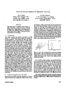
17.1 Introduction A time series is an ordered sequence of observations made through time, whereas a time series prediction problem is the prediction of future data R(t0 + h) at horizon h > 0, given historical data R(t), t = 1, · · · , t0 , in the form of a vector or a scalar. Time series predictions have been used in many areas of science, industry, and commercial and financial activities, such as financial forecasts on stock prices and currency exchange rates, product sale and demand forecasting, population growth, and earthquake activities. In general, a time series may exhibit nonlinearity, non-stationarity, and possibly periodic behavior such as seasonality. More often than not, observations were contaminated by noise that makes a time series noisy. Figure 17.1 illustrates a noisy nonstationary periodic time series. These four characteristics are described as follows. 1. Linearity. A time series is linear if R(t + h) can be expressed as a linear function of some or all of its historical values f (R(t), R(t − 1), · · ·); otherwise, it is nonlinear. In this chapter, we are interested in developing general models that can represent nonlinear time series with a continuous function f .

404

B.W. Wah and M.L. Qian 16 14 12

periodicity

10 8

noise

6

nonstationarity

4 2 0 −2

0

10

20

30

40

50

60

70

80

90

100

Fig. 17.1. An example of a nonstationary, periodic and noisy time series

2. Stationarity. A time series is stationary if it has constant mean and variance; otherwise, it is nonstationary. Nonstationarity is hard to model, as its future behavior may be unpredictable. In this chapter, we are interested in stationary time series as well as a special class of nonstationary time series called piecewise chaotic time series. A time series is piecewise chaotic if it consists of several regimes in which each regime corresponds to a chaotic process, and the overall time series is a collection of multiple chaotic regimes. 3. Periodicity. A time series with dominant periodic components will exhibit regular periodic variations. Such behavior is displayed, for example, in annual electricity consumption and merchandise sales. Since periodicity is a well studied property and can be eliminated effectively by differencing techniques [17.7], we do not consider it in this chapter. 4. Random noise can be present in the entire or some parts of the frequency spectrum of a time series. Since random noise cannot be predicted, we only study time series with high frequency noise and the prediction of their low frequency components. In the next section, we survey briefly existing work for handling nonlinearity, piecewise chaos and noise in time series. Section 17.3 discusses our newly proposed constrained formulations, along with our violation-guided backpropagation developed to solve the constrained formulations. Section 17.4 presents methods to handle noisy time series using constrained formulations, and illustrates them on the prediction of the low-frequency components of stock prices. Finally, conclusions are drawn in Sect. 17.5.

17.2 Previous Work in Time Series Modeling A variety of time series models have been proposed and studied in the last four decades. In this section, we review briefly some existing models and present their potential problems when applied to handle nonlinear piecewise chaotic time series with and without noise.

17. Constraint-Based Neural Network Learning

405

Time Series Models Nonlinear Models

Linear Models

ARMA & variants [17.4]

state−space models [17.1]

General nonlinearity (Machine learning)

Pre−defined nonlinearity

TAR bilinear AR [17.43] [17.16] Statistic Unsupervised time−varying parameter models Reinforcement [17.39] clustering [17.24]

kNN [17.11] Q−learning [17.53]

Supervised Decision tree learning [17.40]

neural network [17.19]

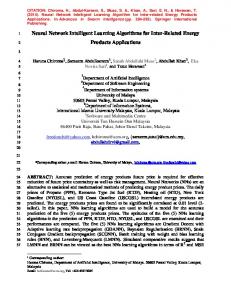
Fig. 17.2. A classification of time-series models for handling nonlinearity

17.2.1 Linearity Figure 17.2 classifies existing time-series models into linear and nonlinear [17.8]. Linear models work well for linear time series but may fail otherwise. There are three types of linear models. 1. Box-Jenkins ARIMA [17.4] and its variations, such as autoregression (AR), moving average (MA), and autoregressive moving average (ARMA), describe future data as a linear combination of historical data and some random processes. 2. Exponential smoothing [17.6] models smoothed data S(t) as a function of raw data R(t) by S(t + 1) = αR(t) + (1 − α)S(t),

0 < α ≤ 1,

(17.1)

where α is the only parameter in the model. 3. State-space models [17.1] represent inputs as a linear combination of a set of state vectors that evolve over time according to some linear equations. Such vectors and their dimensions are usually hard to choose in practice [17.8]. Nonlinear models can be classified into models with predefined nonlinearity assumptions and general models. The first class includes bilinear autoregression [17.16], time-varying parameter models [17.39], and threshold autoregressive models [17.43]. They are not effective for modeling time series with unknown nonlinear behavior. Machine learning can handle nonlinear time series because it learns a model without nonlinearity assumptions. Specific methods that can model temporal sequences include statistic learning (such as k-nearest-neighbors (kNN) [17.11]), reinforcement learning (such as Q-learning [17.53]), unsupervised learning (such as clustering methods [17.24]), and supervised learning (such as decision trees [17.40] and artificial neural networks (ANNs) [17.19]).

406

B.W. Wah and M.L. Qian

In general, these methods learn using a single nonlinear objective on a training set. As a result, they do not use individual patterns to help escape from local optima, especially when gradient-based methods are used [17.42, 17.45]. In this chapter, we propose constrained formulations for ANN learning that add constraints on individual patterns and that use violated constraints to help guide learning. Such formulations are general and can be applied to other learning methods. 17.2.2 Piecewise Chaos Time series with piecewise chaotic regimes have been studied extensively. One approach is to identify local regimes first, before performing learning/predictions on each identified regime. Models using this approach include regime switching models [17.10] and hidden Markov Models [17.26, 17.27]. These approaches are limited because they do not work well unless the changeover points can be correctly identified, and the prediction of changeover points may be as hard as the prediction problem itself. Without separating the process into two steps, machine learning can learn regime changes by reserving patterns in each regime change to be verified in a cross-validation set. However, traditional learning approaches using a single objective may have difficulties in handling cross validations for multiple regime changes because the single objective containing the sum of the errors in all the cross-validation sets does not provide guidance for refinements when it exceeds a preset threshold. To address this issue, a formulation can be used to constrain the error in each validation set to be satisfied during learning. We show such an approach later, applied to ANN learning and its successful prediction of regime changes in testing.

R(t+L)

q −1 g(-L)

R(t+L-1)

q −1

R(t+L-2) g(-L+2)

g(-L+1)

+

+

q −1

R(t-L) g(L)

+

S(t)

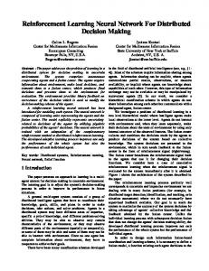
Fig. 17.3. A symmetric FIR filter with 2L taps

17.2.3 Random Noise Random noise is uncorrelated, has zero mean, and is not predictable due to its uncorrelated nature. As its presence in a time series distracts a model from learning useful clean information, especially when the signal-to-noise ratio is relatively low, it is always desirable to eliminate noise before learning.

17. Constraint-Based Neural Network Learning

407

Autocorrelations 1

54 52

0.9

50 48

0.8

46 44

low pass

0.6

40 38

0.5

36 34

1.2

55

0.7

42

32

0.4 0

100

150

Lag by 10 days

0.8 45 0.6

high pass

40 0.4 35 0.2 30

50

0

0

50

100

150

200

IBM stock prices

0

Today

1

0.3

0.8

0.2

0.6 0.5

1

1.5

2

2.5

3

3.5

Frequency responses of a 20−tap FIR filter bank

10

15

20

15

20

lag period

0.1

0.4 0

5

200

1

50

0

0.2 −0.1

0

−0.2

−0.2

−0.3

−0.4 −0.6 −0.8

−0.4

0

50

100

150

0

5

10

200

lag period

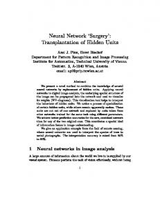
Fig. 17.4. An illustration of a filtering process on a time series of noisy IBM daily closing prices using a 20-tap symmetric low-pass FIR filter to de-noise the time series. Both the low-pass and high-pass data have a 10-day lag. The right two panels show the autocorrelation plots for both filtered time series

In the literature, de-noising is usually done by low-pass filtering or wavelet transforms [17.33, 17.58]. Figure 17.3 illustrates the use of a symmetric FIR filter to generate de-noised data S(t): S(t) =

L X

R(t + l)g(j),

(17.2)

j=−L

where g(j) is the j th filter coefficient, 2 L is the number of filter taps, and R(t) is the raw data in the noisy time series. A symmetric FIR filter is a non-causal filter because its current filtered output depends on future inputs. For example, the filtered output of a 2Ltap symmetric filter ends at t0 − L because it depends on raw data that ends at t0 . Such dependencies on future data lead to a lag (sometimes called an edge effect) in the filtered data. Figure 17.4 shows a 10-day lag in both the low-pass and high-pass data of the closing stock prices of IBM, when filtered by a 20-tap symmetric FIR filter. The edge effect is not a unique artifact of non-causal filters but also occurs when causal filters are used. Although the outputs of causal filters do not depend on future inputs, they reflect a delayed behavior of the original time series and amount to a lag similar to that in non-causal filters. To overcome edge effects in a time series, a predictor has to first predict missing filtered data in the lag period before predicting into the future. In a time series with high frequency random noise, such predictions will be limited to those of low-pass data, as the autocorrelations between high frequency samples at distances longer than the lag period will be low (Fig. 17.4). As a result, we focus on the predictions of low-pass data in this chapter. Existing approaches on predicting missing low-pass data in a lag period typically impose some assumptions on the future raw data. Figure 17.5 show some example approaches [17.33, 17.38, 17.57]. Here, flat extension assumes

408

B.W. Wah and M.L. Qian Mirror extension

Wraparound

Zero extension

Flat extension

0

Average absolute errors

Fig. 17.5. Four techniques for handling edge effects in order to compensate for missing data in the lag period. Solid lines represent actual raw data, and dashed lines stand for extended data 1.2

Mirror extension Flat extension

1 0.8 0.6 0.4 0.2 0 1

2

3

4 5 6 7 8 Day index in the lag period

9

10

Fig. 17.6. The average absolute errors diverge quickly when predicting missing low-pass data in the lag period of ten days

that future raw data R(t0 +j), j = 1, 2, . . . , is the same as the latest observed raw data R(t0 ); mirror extension assumes that future raw data is a mirror image of history data, that is, R(t0 +j) = R(t0 −j +1); wrap-around assumes that after a period of T , the time series repeats itself; and zero extension assumes future data R(t0 + j) to be zero. Using the extended raw data, lowpass filtering is then applied to obtain the de-noised data in the lag period. In this chapter, we do not consider wrap-around and zero extension, as they are applicable only when the time series is stationary and has zero mean. Figure 17.6 shows the mean absolute errors between the true low-pass data of the closing stock prices of IBM and its corresponding predicted lowpass data using flat and mirror extensions. Although flat extension performs slightly better than mirror extension in this case, both show that the average errors of low-pass data in one part of the lag period (specifically, the last three days) are considerably larger than those in the rest of the lag period. As the low-pass values in the first seven days of the lag period are quite accurate, they can be used as training patterns as if they were true low-pass values. In our approach described in Sect. 17.4.2, we use de-noised data in the first part of the lag period as training patterns, and predict patterns in the latter part of the lag period and beyond. We further use constraints on the raw data in the lag period in order to have more accurate predictions in the lag period.

0.08

0.8

0.06

0.4

Pattern Error

MSE

17. Constraint-Based Neural Network Learning

0.04 0.02 0

409

target training training error

0 -0.4 -0.8

0

2000 4000 6000 Number of Training Iterations

8000

0

50

100 150 Pattern Number

200

b) Training errors on individual patterns after 2000 iterations Fig. 17.7. Sunspots time series trained by backpropagation using an unconstrained formulation of (17.3) a) Progress of mean squared errors

17.2.4 Artificial Neural Networks It is well known that ANNs are universal function approximators and do not require knowledge of the process under consideration. ANNs for modeling time series generally have special structures that store temporal information either explicitly, using time-delayed structures, or implicitly, using feedback structures. Examples of the first class include timedelayed neural networks (TDNNs) [17.29] and FIR neural networks (FIRNN) [17.51, 17.52], whereas examples of the latter include recurrent neural networks (RNNs) [17.13, 17.55]. Other architectures, such as radial-basis function network (RBF) [17.36] and supporting vector machines [17.37], store approximate history information in either radial-basis functions or the socalled supporting vectors. Time-series predictions using ANNs have traditionally been formulated as unconstrained optimization problems that minimize the mean squared errors (MSE) defined as follows: min E(w) = w

No n X X

(oi (t) − di (t))2

(17.3)

t=1 i=1

where No is the number of output nodes in the ANN, o(t) and d(t) are, respectively, the actual and desired outputs of the ANN at time t, w is a vector of all the weights, and the training data consists of patterns observed at t = 1, · · · , n. Extensive past research has been conducted on designing learning algorithms using an unconstrained formulation in order to lead to ANNs with a small number of weights that can generalize well. However, such learning algorithms have limited success because little guidance is provided in an unconstrained formulation when a search is stuck in a local minimum of the weight space. In this case, the unconstrained objective in Eq. (17.3) does not indicate which patterns are violated and the best direction for the trajectory to move.

410

B.W. Wah and M.L. Qian

Figure 17.7 illustrates the lack of guidance when an unconstrained formulation is used. In this example, an ANN was trained by backpropagation to predict the Sunspot time series. Figure 17.7a shows that the MSE in training decreased quickly in the first 1,000 iterations but had little improvement after 2,000 iterations. Further examination of the weights shows that they were almost frozen after 2,000 iterations, and the gradients in all the iterations thereafter were very small. Yet the pattern errors in Fig. 17.7b shows that there were still considerably large errors for some patterns, and that these violated patterns were not identified in an unconstrained formulation. To this end, we propose in the next section a constrained formulation with a constraint on each pattern, and an efficient algorithm for searching in constrained space. Besides minimizing training errors, cross validations have been used to prevent overfitting in ANN training. Traditional learning involving cross validations generally divides the available historical data into two disjoint training and validation sets and uses the MSE of the validation set as the sole objective. The reason for using only one validation set is due to the limitation of unconstrained formulations that can handle only one objective function. A problem faced in traditional validations is in choosing a proper crossvalidation set. Although there is no defined way on how long and where the validation set should be, one prefers to reserve the last portion of the historical data for validation in order for the ANN to generalize well into the future. Since the training and validations sets are disjoint, the use of the last portion of patterns as a validation set prevents them from being used as training patterns. As a result, the ANN learned does not have access to the most recent patterns in a time series, which are usually the most important for predicting into the future. This is a dilemma in traditional cross validations used in time series predictions. Another problem faced in traditional validations is related to piecewise chaotic time series. Since piecewise chaotic time series behave differently at changeover points, these points need to be learned specifically in order for the learned system to generalize well. For example, the Laser time series [17.54] in Fig. 17.8 is a piecewise chaotic time series with two changeover points at 180 and 600, respectively. To learn these changeover points, we like to have one validation set at the segment around 600 and another at the segment around 1,000, right before the end of the training set. Such multi-objective learning cannot be handled by traditional single-objective formulations, but can be modeled in a constrained formulation that considers the error of each cross-validation set as an additional constraint. In the rest of this chapter, we describe ANN solutions for predicting time series. We first present, in the next section, constrained formulations and learning algorithms for accurately predicting stationary and piecewise chaotic nonlinear time series. We then present, in Sect. 17.4, the design of efficient

17. Constraint-Based Neural Network Learning

411

Fig. 17.8. Laser is a piecewise chaotic time series that requires at least two validation sets: one for the regime changeover section and another at the end of training

learning algorithms for predicting missing low-pass data of noisy time series in the lag period and beyond.

17.3 Predictions of Noise-Free Stationary and Piecewise Chaotic Time Series The predictions of a noise-free time series by an ANN are generally carried out by single-step (or iterative) predictions in which the inputs to the ANN in each prediction step are the true observed (or predicted) outputs of the previous prediction step. In both approaches, we adopt a widely used evaluation metric, the normalized mean square error (nM SE), defined as follows: nM SE =

t1 1 X (o(t) − d(t))2 , σ 2 N t=t

(17.4)

0

where σ 2 is the variance of the true time series in period [t0 , t1 ], N is the number of patterns tested, and o(t) and d(t), respectively, are the actual and desired outputs at time t. In this section, we describe the recurrent FIR ANN architecture used, the constraints developed, the learning algorithm, and our experimental results. 17.3.1 Recurrent FIR Neural Networks Although a variety of ANN architectures for modeling time series have been studied in the past, there was no consensus on the best architecture to use. For example, Horne and Giles concluded that “recurrent networks usually did better than TDNNs except on the finite memory machine problem” [17.23]. Yet, Hallas and Dorffner stated that “recurrent neural networks do not seem

412

B.W. Wah and M.L. Qian

w(0) x(t)

q −1 q −1

q −1

Unit delay +

q −1

w(1)

x(t − 1)

q −1

recurrent node

y(t)

+

w(2)

x(t)

regular node

x(t − 2)

FIR filter

x(t + 1)

q −1

a) Recurrent FIR ANN

+

Bias node with input 1

w(T )

x(t − T )

b) FIR filter

Fig. 17.9. Structure of a three-layer RFIR: Double concentric circles in (a) indicate recurrent nodes; other circles are non-recurrent nodes; and small boxes are bias nodes with constant input 1. q −1 is a one unit time delay

to be able to do so (prediction) under the given conditions” and “a simple feedforward network significantly performs best for most of the nonlinear time series”[17.18]. However, many do agree that the best architecture is problem dependent and that “the efficiency of the learning algorithm is more important than the network model used” [17.28]. Since neither recurrent nor non-recurrent ANNs are found to be superior, we propose a hybrid recurrent ANN called recurrent FIR neural network (RFIR). In RFIR, each feedback link has a non-zero delay, and the link between any two nodes has an explicit memory modeled by a multi-tap FIR filter (Fig. 17.9b) for storing history information. Figure 17.9a shows a simple three-layer RFIR in which each feedback link has an associated unit delay. The advantage of this architecture is that it can store more historical information than both RNN and FIR-NN. The concept of RFIR can be generalized easily to existing recurrent ANNs, such as Elman’s neural network [17.13], fully recurrent neural networks (FRNN) [17.19], and nonlinear autoregressive networks with exogenous inputs (NARX) [17.9]. 17.3.2 Constrained Formulations for ANN Learning A constrained formulation consists of a learning objective, similar to (17.3) used in a traditional unconstrained formulation, and multiple constraints, each enforcing a learning criterion. We describe two types of constraints considered, although others may be added as needed.

17. Constraint-Based Neural Network Learning

Training Set V1

V2

change of regime

413

Test Set V3 end of training

Fig. 17.10. Three validation sets V1 , V2 and V3 defined in a training set. Validation sets V1 and V2 can be used to cover regime changes in a piecewise chaotic time series

Constraints on individual patterns. To address the lack of guidance in search, we have recently proposed new constraints that account for the error on each training pattern in a constraint [17.45, 17.46, 17.47, 17.48, 17.49]. The resulting optimization problem is as follows: minw

E(w) =

No n P P t=1 i=1

φ((oi (t) − di (t))2 − τ )

(17.5)

subject to hi (t) = (oi (t) − di (t))2 ≤ τ for all i and t, where φ(x) = max{0, x}. Constraint hi (t) ≤ τ prescribes that the error of the ith output unit on the tth training pattern be less than τ , a predefined small positive value on the learning accuracy to be achieved. Note that E(w) is modified from (17.3) in such a way that when all the constraints are satisfied, the objective will be zero and learning stops. A constrained formulation is beneficial in difficult training scenarios because violated constraints provide additional guidance during a search, leading a trajectory in a direction that reduces overall constraint violations. It can overcome the lack of guidance in Fig. 17.7 when the gradient of the objective function in an unconstrained formulation is very small. A search algorithm solving a constrained formulation has information on all pattern errors and on exactly which patterns have large errors. Hence, it may intentionally modify its search direction by increasing gradient contributions from patterns with large errors. Constraints on cross validations. Our constrained formulation leads to a new method for cross validations [17.46], shown in Fig. 17.10, that defines multiple validation sets in learning and that includes the error from each validation set in a new constraint. The validation error for the ith output unit from the k th , k = 1, · · · , v, validation set is accounted for by nM SE in both singlestep and iterative validations. The advantage of this new approach is that training can be performed on all historical data available, without excluding validation patterns from training as in previous approaches. It considers new constraints on errors in iterative validations, thereby avoiding overfitting of the ANN learned. Further, it allows a new validation set to be defined for each regime transition region in the training data of a piecewise chaotic time series, leading to more accurate predictions of regime changes in the future. Denote the iterative (or single-step) validation-constraint function for the ith output node in the k th validation set as hIk,i (or hSk,i ). The constrained

414

B.W. Wah and M.L. Qian

formulation of (17.5) becomes minw Eav (t0 , t1 ) =

No t1 P P t=t0 i=1

φ((oi (t) − di (t))2 − τ )

subject to hi (t) = (oi (t) − di (t))2 ≤ τ, I hIk,i = eIk,i ≤ τk,i , S S S hk,i = ek,i ≤ τk,i ,

(17.6)

where eI (or eS ) is the nM SE of the iterative (or single-step) validation I S error, and τk,i and τk,i are predefined small positive constants. Eq. (17.6) is a constrained nonlinear programming problem (NLP) with non-differentiable function hIk,i . Hence, existing Lagrangian methods that require the differentiability of functions cannot be applied. Existing methods based on penalty formulations have difficulties in convergence when penalties are not chosen properly. Yet, algorithms that sample in real space and that apply the recently developed theory of Lagrange multipliers for discrete constrained optimization [17.50, 17.56] are too inefficient for solving large problem instances. To this end, we describe next an efficient learning algorithm called violation-guided backpropagation (VGBP) [17.47, 17.48]. 17.3.3 Violation-Guided Backpropagation Algorithm Assuming that w is discretized, we first transform (17.6) into an augmented Lagrangian function: ¶ No µ n X X 1 L(w, λ) = E(w) + λi (t)φ(hi (t) − τ ) + φ2 (hi (t) − τ ) (17.7) 2 t=1 i=1 ¶ No µ v X X X 1 j j λjk,i φ(hjk,i − τk,i ) + φ2 (hjk,i − τk,i ) . + 2 i=1 j=I,S k=1

The discretization of w will result in an approximate solution to (17.6) because a discretized w that minimizes (17.6) may not be the same as the true optimal w. With fixed error thresholds, (17.6) may not be feasible with a discretized w but feasible with a continuous w. This is not an issue in ANN learning using (17.6) because error thresholds in learning are adjusted from loose to tight, and there always exist error thresholds that will lead to a feasible discretized w. According to the theory of Lagrange multipliers for discrete constrained optimization [17.50], a constrained local minimum in the discrete w space of (17.6) is equivalent to a saddle point in the discrete w space of (17.7), which is a local minimum in the w subspace and a local maximum in the λ subspace. To look for the saddle points of (17.7) by performing descents in the w subspace and ascents in the λ subspace [17.44], we have proposed in Fig. 17.11 the violation guided back-propagation algorithm [17.47, 17.48].

17. Constraint-Based Neural Network Learning

Start

E) Initailizations: candidate point and λ; set initial parameters

w loop

Y N Stop training and do prediction

F) Reset parameters? using R&T

Search in λ subspace

B) Accept candidate point (annealing rules)

A) Generate new candidates in the w subspace (gradient-based by BP)

N

N Stopping conditions met?

Y

415

C) Generate new candidate in the λ subspace (greedy rules)

λ loop D) Update Lagrangian values (deterministic rules)

Y

Fig. 17.11. VGBP: an iterative search procedure employing relax-and-tighten (R&T) to solve a discrete constrained formulation for ANN time-series predictions. The shaded box represents the routine to look for saddle points in discretized w subspace and continuous λ subspace

The λ loop carries out ascents in the λ subspace by generating candidates in that subspace in Box (C) and by accepting them using deterministic rules in Box (D). Box (C) increases λ if the violation of the corresponding constraint is found to be larger than a certain threshold. In this way, a training pattern with a large error will have a larger Lagrange multiplier λ. For a learning problem with a large number of weights and/or training patterns, it is essential that the points generated in Box (A) be likely candidates to be accepted in Box (B). Since (17.7) is not differentiable, we compute an approximate gradient direction by ignoring single-step and iterative validation errors in (17.6) and use BP [17.48] to find the gradient of Pn PNo the approximate Lagrangian function t=1 i=1 (1 + λi (t))(hi (t) − τ ). We then generate a trial point using the approximate gradient and step size η. In this way, a training pattern with a large error will contribute more in the overall gradient direction because of its larger Lagrange multiplier, leading to an effective suppression of constraint violations. Since the gradient direction computed by BP is based on a heuristic step size and does not consider constraints due to cross validations, a search based on that direction may not always lead to a reduced Lagrangian function value and may get stuck in infeasible local minima of the w subspace. Although restarts can help escape from those local minima, our experimental results have shown that uncontrolled restarts from those points may lead to the loss of valuable local information collected during a search. To address this issue, we propose an annealing strategy in Box (B) that decides whether to go from current point (w, λ) to (w0 , λ) according to the Metropolis probability [17.47, 17.48] n o 0 + )) AT (w0 , w)|λ = exp (L(w)−L(w , (17.8) T where x+ = min{0, x}, and T is introduced to control the acceptance probability. Tolerances τ, τ I and τ S are set by the relax-and-tighten strategy proposed in [17.47]. This strategy is based on the observation that looser constraints are easier to satisfy, while achieving larger violations at convergence, and that tighter constraints are slower to satisfy, while achieving smaller violations at

416

B.W. Wah and M.L. Qian

Table 17.1. Single-step and iterative test performance of VGBP in nM SE on Laser as compared to other published results. The test set consists of patterns from 1,001 to 1,100. As a comparison, we also show the test performance on patterns from 1001 to 1050. Boxed numbers indicate the best results; N/A stands for data not available. Both runs of VGBP were done on an RFIR with one input node, 20 hidden nodes, one output node, feedbacks from output to hidden layers and from hidden to input layers, but without RFIR on each link Method

# of weights

FIR1105 NN [17.52] ScaleNet N/A [17.15] VGBP 461 (Run 1) VGBP 461 (Run 2)

0.00044

Single-step 10011050 0.00061

predictions 10011100 0.023

Iterative predictions 100110011050 1100 0.0032 0.0434

0.00074

0.00437

0.0035

N/A

0.00043

0.0034

0.0054

0.00036

0.00107

250 Laser Intensity

Training 100-1000

0.00030

0.00276

N/A

0.0030

0.0194

0.0294

expected intensity predicted intensity

200 150 100 50 0 1000

1020

1040

1060

1080

1100

Pattern Index in Iterative Predictions

Fig. 17.12. Iterative predictions starting at Pattern 1001 made by an ANN trained by VGBP on a constrained formulation (Run 1 in Table 17.1)

convergence. By using loose constraints at the beginning and by tightening the constraints gradually, learning converges faster with tighter tolerances. 17.3.4 Experimental Results We have tested our formulations and algorithms on several benchmarks, including Laser, Sunspots, and five chaotic time series. We present only partial results here [17.46, 17.47, 17.48]. Laser is taken from the Sante Fe time series competition [17.54], in which Wan’s FIR-NN [17.52] won the first place on this time series. Table 17.1 shows that VGBP improves Wan’s result in terms of both single-step and iterative

17. Constraint-Based Neural Network Learning

417

Table 17.2. A comparison of single step-prediction performance in nM SE on five methods: Carbon copy (CC), linear [17.52], FIR-NN [17.52], DRNN [17.2], and VGBP. Carbon copy simply predicts the next time-series data to be the same as the proceeding data (x(t + 1) = x(t)). The training (resp. testing) set shows the patterns used in learning (resp. testing). Lorenz attractor has two data streams labeled by x and z, respectively, whereas Ikeda attractor has two streams – real (Re(x)) and imaginary (Im(x)) parts of a plane wave Bench- TrainingTestingPerformance Mark

Set

MG17 1500 MG30 1500 Henon 15000

Lorenz 14000

Set

Metrics

CC

501-

nM SE

0.6686

Linear FIRDRNN VGBP NN 0.320 0.00985 0.00947 0.000057

2000 501-

# of weights nM SE

0 0.3702

N/A 0.375

196 0.0279

197 0.0144

121 0.000374

2000 # of weights 5001nM SE

0 1.633

N/A 0.874

196 0.0017

197 0.0012

121 0.000034

10000 # of weights 4001- nMSE x

0 0.0768

N/A 0.036

385 0.0070

261 0.0055

209 0.000034

5500

0.2086

0.090

0.0095

0.0078

0.000039

0 2.175

N/A 0.640

1070 0.0080

542 0.0063

527 0.00023

1.747

0.715

0.0150

0.0134

0.00022

0

N/A

2227

587

574

z

# of weights 10001-nMSE Re(x) Ikeda

Design Methods

111500 10000

Im(x) # of weights

predictions, using less than half of the weights. Figure 17.12 further shows that VGBP gives accurate iterative predictions for over 60 steps, predicting precisely the regime changeover point and some phase shift afterwards. We have also tested five more nonlinear chaotic time series: Mackey-Glass 17 (MG17), Mackey-Glass 30 (MG30), Henon, Lorenz, and Ikeda. Table 17.2 compares our results with four other predictors and shows that our ANNs trained by VGBP on constrained formulations use less weights and achieve nM SEs that are one to two orders of magnitude smaller.

17.4 Predictions of Noisy Time Series with High Frequency Random Noise As most financial time series have been found to be noisy and behave like random walks [17.12, 17.58, 17.22], we use daily closing stock prices as ex-

418

B.W. Wah and M.L. Qian

amples of noisy time series to illustrate how such series can be learned using constrained formulations. As mentioned earlier, a de-noised low-pass filtered time series lags behind the original series, and a predictor needs to predict the missing low-pass data in the lag period before predicting into the future. 17.4.1 Review on Financial Time Series Predictions Models for financial time-series forecasting can be classified into linear, nonlinear, and expert system-based. Linear models are still popular in financial time-series predictions, the most popular of which are exponential smoothing, ARIMA models [17.31, 17.32, 17.35, 17.25], and GARCH models (linear in mean and nonlinear in variance) [17.5, 17.34]. Nonlinear models consist mainly of the k-nearest-neighbor methods and ANN methods [17.3, 17.34, 17.41]. Expert systems employ a collection of models (including exponential smoothing methods, ARIMA methods, and moving average), develop a set of rules for selecting a specific method [17.14, 17.35], and select one method for activation when certain conditions are satisfied. In the past twenty years, there were three Makridakis competitions (also known as M-Competitions [17.30], M2-Competitions [17.31], and M3Competitions [17.32]) held to test forecasting accuracy, including financial and economic time series. A variety of models, including those aforementioned, were tested. The conclusions reached were rather consistent. We list below some related conclusions drawn from these competitions and the literature [17.17, 17.21, 17.34]. – No single method is clearly superior to other methods in most time series tested. – Existing methods do not outperform random walk models significantly and statistically in terms of both prediction accuracy and prediction directions (up/down trends). In some cases, they are even worse than random walks. – Prediction quality is measurement dependent. 17.4.2 Constraint in the Lag Period In our approach, we first apply flat extensions to generate future raw time series data, obtain low-pass data in the first part of the lag period using the extended raw data, and train an RFIR by VGBP, while including the low-pass data in the first part of the lag period as learning patterns and as additional constraints on raw data . After the RFIR is trained, we use it to predict low-pass data in the latter part of the lag period and into the future. In order to improve prediction accuracy, we include a special constraint in the lag period by utilizing the available raw data. Let R(t) be the raw data, ˆ S(t) be the low-pass data, and S(t) be the ANN output at time t (where t can occur during learning or during prediction). Since the low-pass curve is a smoothed version of the raw data curve, the raw data in the lag period

Low−frequency filtering ended

17. Constraint-Based Neural Network Learning

PRICE

419

Low frequency target Network output Actual raw data

DAY Today Lag

Fig. 17.13. Illustration of an additional constraint in the lag period. The raw data should center around the low-pass data as well as the ANN outputs iterative predictions

training

t0 +1

t0 -10 t0 -3

Fig. 17.14. Predictions beyond the lag period using a 20-tap filter

generally centers around the true low-pass curve and, consequently, the curve of the ANN outputs (Fig. 17.13). This observation motivates us to add a new constraint in (17.6) on the difference between the raw data and the ANN outputs in the lag period: hlag =

t0 X

ˆ − R(t) ≤ τ lag . S(t)

(17.9)

t=t0 −m+1

The new constrained formulation for ANN learning of noisy time series can now be solved by VGBP. 17.4.3 Experimental Results We have conducted experiments by low-pass filtering of time series using a 20-tap filter that incurs a 10-unit lag. After extending the raw data by flat extensions and low-pass filtering of the extended data, we have found experimentally that the last three low-pass values in the lag period have considerably large errors (Fig. 17.6). Figure 17.14 shows the use of the first seven low-pass values in the lag period in training RFIR and the iterative predictions from t0 − 2. True predictions start from t0 + 1. To test whether our approach will lead to more accurate predictions on future data, we have used the daily closing prices of IBM (symbol IBM), Citigroup (symbol C) and Exxon-Mobil (symbol XOM) between April 1, 1997

420

B.W. Wah and M.L. Qian

and March 31, 2002. We have also constructed the following five predictors: CC: AR(30): NN:

LNN:

IP:

Carbon copy that simply copies the most recently available data; Autoregression with an order of 30, using the TISEAN implementation [17.20]; Unconstrained formulation trained by BP on RFIR with one input node, two hidden nodes, one output node, feedbacks from hidden to input layers and from output to input layers, and one-tap FIR structure on each feedback link; Constrained formulation, with constraints on the lag period and using seven predicted data values in the lag period, trained by VGBP using the same RFIR structure as NN; Ideal predictor, same as LNN but using seven true values in the lag period.

IP establishes an approximate upper bound for prediction accuracy, as it uses seven error-free low-pass data in the lag period that are not available otherwise. To compare prediction accuracy, we use nM SE, as well as the widely used metric called hit rate in financial time series predictions. Let D(t + h) = sign(S(t + h) − S(t)) be the actual direction of change for S(t), and let ˆ + h) = sign(S(t ˆ + h) − S(t)) ˆ D(t be the predicted direction change. We call ˆ + h) × D(t + h) > 0, and a prediction for horizon h a hit if and only if D(t we define the hit rate H(h) as follows: ¯ ¯ ¯ ˆ + h) > 0}¯¯ ¯{t where D(t + h)D(t ¯, t = 1, · · · , n, (17.10) H(h) = ¯¯ ˆ + h) 6= 0}¯¯ ¯{t where D(t + h)D(t where |E| represents the number of elements in set E. Figure 17.15a shows the nM SEs of the five predictors for the period between April 1, 1997, and March 31, 2002. (Predictions did not start on April 1, 1997, as an initial window of 200 days were used for training before the first prediction was made.) AR(30) and NN do not perform well because they need to predict iteratively in the 10 day lag period before predicting into the future. LNN improves significantly over CC and AR(30), especially for small horizons, and outperforms traditional NN over all horizons. It also shows that LNN has errors closest to those of IP over small prediction horizons, and achieves slightly better nM SE at longer horizons. (Note that IP only gives an approximate upper bound on accuracy.) Figure 17.15b plots the hit rates for the five predictors. It shows that CC, AR(30) and NN behave like random walks over the 10 day horizons, as they always have around a 50% chance to predict the correct direction of price

17. Constraint-Based Neural Network Learning Citigroup

CC AR(30) NN LNN IP

0

Rate %

nMSE

Citigroup 0.3 0.25 0.2 0.15 0.1 0.05 0

2

4

6

8

75 70 65 60 55 50 45 40

CC AR(30) NN LNN IP

0

10

2

4

nMSE

0.7 0.6 0.5 0.4 0.3 0.2 0.1 0

Rate %

CC AR(30) NN LNN IP

0

2

4

6 Horizon Exxon Mobil

8

2

4

6 Horizon

8

75 70 65 60 55 50 45

8

10

10

CC AR(30) NN LNN IP

0

10

CC AR(30) NN LNN IP

0

6 Horizon IBM

Rate %

nMSE

Horizon IBM 0.6 0.5 0.4 0.3 0.2 0.1 0

421

2

4

6 Horizon Exxon Mobil

80 75 70 65 60 55 50 45

8

10

CC AR(30) NN LNN IP

0

2

4

6

8

10

Horizon

a) nM SE b) Hit rate Fig. 17.15. Performance of five predictors tested on the daily closing prices of Citigroup, IBM and Exxon-Mobil

changes. On the other hand, LNN can achieve hit rates significantly higher than 50% over small horizons (one to five days). Finally, IP performs better than LNN for small horizons (one to five days), but performs statistically the same as LNN for large horizons (six days and beyond). Figure 17.16 plots the predictions of LNN on the next day closing prices of IBM over 1,100 days, as compared to the actual low-pass data. The results show that the predictions track well with the actual low-pass data. Finally, we analyze the probability that a random walk can achieve the same level of prediction accuracy as LNN, and conclude that it is very unlikely that LNN is a random walk. Since a random walk has a probability of p = 0.5 to achieve a hit for each prediction, the probability for it to achieve k hits out of n predictions is governed by a binomial probability: n! Prob(Hits = k|n predictions) = pk (1 − p)n−k k!(n − k)! n! = 0.5n . (17.11) k!(n − k)! It can be shown that the probability for a random walk to achieve 660 hits in 1,100 predictions (hit rate of 0.6) is only 1.15 × 10−11 , and that the probability for it to achieve more than 605 hits (hit rate of 0.55) is 4.05 × 10−4 .

422

B.W. Wah and M.L. Qian 140

Price

120 100 80 Low-pass target Prediction

60 40 0

200

400

600 Day Index

800

1000

Fig. 17.16. Next-day predictions on IBM’s low-pass daily closing prices

Hence, it is very unlikely that a random walk can achieve the same level of prediction accuracy as LNN. Further, considering that results in the literature on financial time series forecasting achieve next day hit rates below 55% [17.17, 17.21, 17.34], our results are very competitive.

17.5 Conclusions We have studied the predictions of noise-free as well as noisy time series using ANNs. For noise-free and possibly piecewise chaotic time series, we have proposed new constrained formulations for ANN learning that allow multiple learning criteria and prior knowledge to be included. Such criteria include testing errors on multiple validation sets that can model regime changes in piecewise chaotic time series, and the error of the ANN learned when validated on the objective used in testing. We have further proposed a new RFIR architecture that combines a recurrent structure and a memory-based FIR structure, and incorporates a violation-guided backpropagation algorithm based on the theory of Lagrange multipliers for discrete constrained optimization. For noisy time series with high frequency random noise, we have studied systematically the edge effect due to low-pass filtering of noisy time series. To predict missing low-pass data in the lag period, we have developed an approach that estimates low-pass values in the lag period using raw data extended by flat extensions, and that incorporates new constraints on predicted low-pass data in the lag period. The new constraints enable active training in the lag period that greatly improves the prediction accuracy in that period.

References 17.1 M. Aoki: State Space Modeling of Time Series (Springer-Verlag, Nerlin, 1987)

17. Constraint-Based Neural Network Learning

423

17.2 A. Aussem: Dynamical recurrent neural networks towards prediction and modeling of dynamical systems. Neurocomputing, 28, 207-232 (1999) 17.3 S.D. Balkin, J.K. Ord: Automatic neural network modeling for univariate time series. Int’l J. of Forecasting, 16, 509-515 (2000) 17.4 G.E.P. Box, G.M. Jenkins: Time Series Analysis: Forecasting and Control, 2nd ed. (Holden-Day, San Francisco, 1976) 17.5 C. Brooks, S.P. Burke, G. Persand: Benchmarks and the accuracy of GARCH model estimation. Int’l J. of Forecasting, 17, 45-56 (2001) 17.6 R.G. Brown: Smoothing, Forecasting and Prediction (Prentice Hall, Englewood Cliffs, NJ, 1963) 17.7 C. Chatfield: The analysis of time series-an introduction (Chapman & Hall, London, 5 edition, 1996) 17.8 C. Chatfield: Time-series forecasting (Chapman & Hall/CRC, Boca Raton, Florida, 2001) 17.9 S. Chen, S. Billings, P. Grant: Non-linear system identification using neural networks. Int’l J. of Control, 51, 1191-1214 (1990) 17.10 D. Drossu, Z. Obradovic: Regime signaling techniques for non-stationary time series forecasting. In: Proc. 30th Hwaii Int’l Conf. on System Sciences (Wailea, HI, USA, 1997) 5, pp. 530-538 17.11 R.O. Duda, P.E. Hart: Pattern Classification and Scene Analysis (John Wiley and Sons, 1973) 17.12 R.D. Edwards, J. Magee: Technical Analysis of Stock Trends (John Magee, Springfield, MA, 5 edition, 1966) 17.13 J.L. Elman: Finding structure in time. Cognitive Science, 14, 179-211 (1990) 17.14 B.E. Flores, S.L. Pearce: The use of an expert system in the M3 competition. Int’l J. of Forecasting, 16, 485-496 (2000) 17.15 A.B. Geva: ScaleNet - multiscale neural-network architecture for time series prediction. IEEE Trans. on Neural Networks, 9 (5), 1471-1482 (1998) 17.16 C.W.J. Granger, A.P. Andersen: Introduction to Bilinear Time Series Models (Vandenhoeck & Ruprect, G¨ oittingen, 1978) 17.17 S. Gutjahr, M. Riedmiller, J. Klingemann: Daily prediction of the foreign exchange rate between the us dollar and the german mark using neural networks. In: Proc. of SPICES pp. 492-498 (1997) 17.18 M. Hallas, G. Dorffner: A comparative study on feedforward and recurrent neural networks in time series prediction using gradient descent learning. In: Proc. of 14th European Meeting on Cybernetics and Systems Research 2, pp. 644-647 (1998) 17.19 S. Haykin: Neural Networks: A Comprehensive Foundation (Prentice Hall, NJ, 2 edition, 1999) 17.20 R. Hegger, T. Schreiber: The TISEAN software package. http://www.mpipks-dresden.mpg.de/ tisean (2002) 17.21 T. Hellstrm: Predicting a rank measure for stock returns. Theory of Stochastic Processes, 6(20), 64-83 (2000) 17.22 T. Hellstrom, K. Holmstrom: Predicting the Stock Market. Technical Report Series IMa-TOM-1997-07, Malardalen University, Vasteras, Sweden, 1997 17.23 B.G. Horne, C.L. Giles: An experimental comparison of recurrent neural networks. In: G. Tesauro, D. Touretzky, T. Leen (eds.), Neural Information Processing Systems (MIT Press, Cambridge, MA, 1995) pp. 697-704 17.24 A.K. Jain, M.N. Murty, P.J. Flynn: Data clustering: A review. ACM Computing Surveys, 31 (3), 264-323 (1999) 17.25 E.S. Gardner Jr., E.A. Anderson-Fletcher, A.M. Wicks: Further results on focus forecasting vs. exponential smoothing. Int’l J. of Forecasting, 17, 287-293 (2001)

424

B.W. Wah and M.L. Qian

17.26 B.H. Juang, L.R. Rabiner: Hidden Markov models for speech recognition. Technometrics, 33, 251-272 (1991) 17.27 J. Kohlmorgen, K.R. M¨ uller, K. Pawelzik: Analysis of drifting dynamics with neural network hidden markov models. Advances in Neural Information Processing Systems, 10 (1998) 17.28 T. Koskela, M. Lehtokangas, J. Saarinen, K. Kaski: Time series prediction with multilayer perceptron, FIR and Elman neural networks. In: Proc. of the World Congress on Neural Networks pp. 491-496 (1996) 17.29 K.J. Lang, G.E. Hinton: The development of the time-delayed neural network architecture for speech recognition. Technical Report #CMU-CS-88-152, Carnegie-Mellon University, Pittsburgh, PA, 1988 17.30 S. Makridakis, A. Andersen, R. Carbone, R. Fildes, M. Hibon, R. Lewandowski, J. Newton, E. Parzen, R. Winkler: The accuracy of extrapolation (time series) methods: results of a forecasting competition. Int’l J. of Forecasting, 1, 111-153 (1982) 17.31 S. Makridakis, C. Chatfield, M. Hibon, M. Lawrence, T. Mills, K. Ord, L.F. Simmons: The M2-Competition: a real-time judgementally based forecasting study. Int’l J. of Forecasting, 9, 5-23 (1993) 17.32 S. Makridakis, M. Hibon: The M3-Competition: results, conclusions and implications. Int’l J. of Forecasting, 16, 451-476 (2000) 17.33 T. Masters: Neural, Novel and Hybrid Algorithms for Time Series Prediction (John Wiley & Sons, Inc., NY, 1995) 17.34 N. Meade: A comparison of the accuracy of short term foreign exchange forecasting methods. Int’l J. of Forecasting, 18, 67-83 (2002) 17.35 G. Melard, J.M. Pasteels: Automatic arima modeling including interventions, using time series expert software. Int’l J. of Forecasting, 16, 497-508 (2000) 17.36 J. Moody, C. Darken: Fast learning in networks of locally-tuned processing units. Neural Computation, 1(2), 281-294 (1989) 17.37 K. M¨ uller, A. Smola, G. R¨ atsch, B. Sch¨ olkopf, J. Kohlmorgen, and V. Vapnik: Predicting time series with support vector machines. In: ICANN pp. 999-1004 (1997) 17.38 F. Murtagh, A. Aussem: Using the wavelet transform for multivariate data analysis and time series forecasting. In: C. Hayashi, H.H. Bock, K. Yajima, Y. Tanaka, N. Ohsumi, Y. Baba, editors, Data Science, Classification and Related Methods pp. 617-624 (Springer-Verlag, 1998) 17.39 D.F. Nicholls, A.R. Pagan: Varying coefficient regression. In: E.J. Hannan, P.R. Krishnaiah, M.M. Rao (eds.), Handbook of Statistics (North-Holland, Amsterdam, 1985) pp. 413-449 17.40 J.R. Quinlan: Induction of decision trees. Machine Learning, 1, 81-106 (1986) 17.41 S. Ramaswamy: One-step prediction of financial time series, BIS Working Paper No. 57. Technical report, Bank for Interal Settlements, Basle, Switzerland, 1998 17.42 Y. Shang, B.W. Wah: Global optimization for neural network training. IEEE Computer, 29, 45-54 (March 1996) 17.43 H. Tong: Nonlinear Time Series: A Dynamical System Approach (Oxford University Press, Oxford, 1990) 17.44 B.W. Wah, Y.X. Chen: Constrained genetic algorithms and their applications in nonlinear constrained optimization. In: Proc. Int’l Conf. on Tools with Artificial Intelligence (IEEE, November 2000) pp. 286-293 17.45 B.W. Wah, M.L. Qian: Constrained formulations for neural network training and their applications to solve the two-spiral problem. In: Proc. Fifth Int’l Conf. on Computer Science and Informatics 1, pp. 598-601 (February 2000)

17. Constraint-Based Neural Network Learning

425

17.46 B.W. Wah, M.L. Qian: Time-series predictions using constrained formulations for neural-network training and cross validation. In: Proc. Int’l Conf. on Intelligent Information Processing, 16th IFIP World Computer Congress (Kluwer Academic Press, August 2000) pp. 220-226 17.47 B.W. Wah, M.L. Qian: Violation-guided learning for constrained formulations in neural network time series prediction. In: Proc. Int’l Joint Conference on Artificial Intelligence (IJCAI, Aug. 2001) pp. 771-776 17.48 B.W. Wah, M.L. Qian: Violation guided neural-network learning fo constrained formulations in time-series predictions. Int’l Journal on Computational Intelligence and Applications, 1(4), 383-398 (December 2001) 17.49 B.W. Wah, M.L. Qian: Constrained formulations and algorithms for stock price predictions using recurrent FIR neural networks. In: Proc. 2002 National Conf. on Artificial Intelligence (AAAI, 2002)(accepted to appear) 17.50 B.W. Wah, Z. Wu: The theory of discrete Lagrange multipliers for nonlinear discrete optimization. Principles and Practice of Constraint Programming, pp. 28-42 (October 1999) 17.51 E.A. Wan: Temporal backpropagation for FIR neural networks. IEEE Int’l Joint Conf. on Neural Networks, 1, pp. 575-580 (San Diego, CA., 1990) 17.52 E.A. Wan: Finite Impulse Response Neural Networks with Applications in Time Series Prediction. Ph.D. Thesis, Standford University, 1993 17.53 C.J. Watkins: Models of Delayed Reinforcement Learning. Ph.D. thesis, Cambridge University (Cambridge, UK, 1989) 17.54 A.S. Weigend, N.A. Gershenfeld (eds.): Time Series Prediction: Forecasting the future and understanding the past (Addison-Wesley, 1994) 17.55 R.J. Williams, D. Zipser: A learning algorithm for continually running fully recurrent neural networks. Neural Computation, 1, 270-280 (1989) 17.56 Z. Wu: The Theory and Applications of Nonlinear Constrained Optimization using Lagrange Multipliers. Ph.D. Thesis, Dept. of Computer Science, Univ. of Illinois, Urbana, IL (May 2001) 17.57 B.L. Zhang, R. Coggins, M.A. Jabri, D. Dersch, B. Flower: Multiresolution forecasting for future trading using wavelet decompositions. IEEE Trans. on Neural Networks, 12, 766-775 (2001) 17.58 G. Zheng, J.L. Starck, J.G. Campbell, F. Murtagh: Multiscale transforms for filtering financial data streams. J. of Computational Intelligence in Finance, 7, 18-35 (1999)