Non-parametric identification of Higher Order Sinusoidal Output ...

Non-parametric identification of Higher Order Sinusoidal Output Describing Functions P. Nuij, M. Steinbuch, O. Bosgra, Eindhoven University of Technology, Department of Mechanical Engineering, Building Wh-1.133, PO Box 513, 5600 MB Eindhoven, The Netherlands. e-mail: [email protected]

Abstract In this paper the concept of the Higher Order Sinusoidal Output Describing Functions (HOSODF) is presented. HOSODF can be defined for the class of causal, stable, time invariant non-linear systems which give a sinusoidal response to a specific harmonic excitation. The HOSODF relate the magnitude and phase of the individual harmonics, which together compose that specific input signal, to the sinusoidal output signal of such a system. HOSODF are the dual of the Higher Order Sinusoidal Input Describing Functions (HOSIDF). Like the HOSIDF, the HOSODF are the results of an extension of linear techniques towards non-linear systems analysis. Using the HOSODF, the non-linear systems under investigation can be modeled as a cascade of the HOSODF and a Virtual Harmonics Compressor (VHC). The VHC is defined as a non-linear component which transforms a harmonic input signal y˘(t) into a sinusoidal output signal y(t) with frequency ω, amplitude a ˆ and phase ϕ. This input signal y˘(t) consists of an infinite amount of harmonics of the output signal y(t) with frequency nω, amplitude a ˆ and phase nω with n = 0, 1, ...∞. Special attention is paid to the non-parametric identification of the HOSODF. The identification requires control of the frequency and amplitude of the sinusoidal output of the system within its domain of possible sinusoidal output signals. This specific state of these non-linear systems can be reached by incorporating the system under test in a feedback loop. In this loop the desired sinusoidal output is defined as the control objective of a dedicated repetitive controller consisting of a memory loop with positive feedback. The design of the learning filter required for stability is also addressed. As a spinoff of the identification technique, the authors see opportunities for advanced non-linear control of shaker systems aimed at sinusoidal excitation of non-linear systems.

1 Introduction In the analysis and synthesis of dynamic systems, frequency domain based techniques are well established. These techniques are based on the concept of the Frequency Response Function (FRF). A limitation of using FRFs is the imperative assumption of linearity of the system behavior. Due to the increasing demands on system performance in for example mechanical positioning systems, non-linear behavior has to be addressed both in the mechanical and the control design. The frequency domain based techniques for the analysis of non-linear systems mentioned in literature can roughly be classified in three groups: • Identification of the linear system In weakly non-linear systems the true linear system can be identified by minimizing the influence of the non-linear distortion using odd multisine excitation signals with minimized crest factor and with an amplitude kept as small as possible [1, 2, 3]. For non-linear systems which can be approximated by Volterra series the Related Linear Dynamic System can be identified using multi-sine based signals [2, 4, 5, 6, 7]. Apart from leakage free measurements, these multi-sine based signals also provide qualitative and quantitative information about the non-linear distortions.

• Identification of the Generalized Frequency Response Function For the class of causal, stable, time-invariant, non-linear systems with fading memory1 , the convolution integral description of the linear system can be generalized to an infinite series called the Volterra series [9, 10, 11]. The n-dimensional Fourier transform of the n-th order Volterra kernel yields the n-th-order FRF, the Generalized Frequency Response Function (GFRF) [12, 13]. GFRFs can be estimated with non-parametric methods if the system can be described by a low order (truncated) Volterra kernel. The high numerical cost however limits these methods to the identification of GFRFs up to a maximum order of three [14, 15]. Parametric identification techniques ease the numerical requirements and allow analytical expressions for GFRFs up to any order [16]. The GFRFs have their limitations: systems with non-fading memory, like non-local memory hysteresis as seen in friction, can not be described with GFRFs and GFRFs are difficult to interpret due to their multidimensional nature [17, 18]. • Describing Functions The Describing Function concept extends the FRF in the way that identification of amplitude dependency becomes possible [19, 20]. Its recently formulated generalization, the Higher Order Sinusoidal Input Describing Functions (HOSIDF) also describes the generation of harmonics as function of excitation frequency and amplitude [21, 22, 23]. The HOSIDF relate the magnitude and phase of individual harmonics in the output signal to the sinusoidal input signal causing this harmonic response. All nonlinear systems with a harmonic response to a sinusoidal excitation can be described with HOSIDF. The HOSIDF are easy to interpret but do not describe non-linear phenomena like desensitization and intermodulation [18, 24, 25]. In this paper the Higher Order Sinusoidal Output Describing Functions (HOSODF) will be introduced. These higher order describing functions are dual to the HOSIDF in the sense that they are based on a sinusoidal output state. The paper starts with the definition of the class of systems under consideration. Subsequently the Virtual Harmonics Compressor is introduced as the dual to the Virtual Harmonics Expander. The mathematical framework of the HOSODF is presented, as well as a practical non-parametric measurement method for HOSODF. For the identification of the HOSODF it is necessary to control the state of the system under test to generate a sinusoidal output as a response to a harmonic excitation. A feedback loop is presented incorporating a repetitive controller able to force a sinusoidal output from that system.

2 Definition of the class of systems under consideration The systems under consideration belong to the class O of causal, stable, time invariant non-linear systems which have a sinusoidal response to a harmonic excitation. This class is a subset of the class I of causal, stable, time invariant non-linear systems which have a harmonic response to a sinusoidal excitation and can be described with HOSIDF. As an example of a system which belongs to class I and not to class O one can think of a system with output saturation. Unless stated otherwise, non-linear systems mentioned in the sequel of this paper are assumed to belong to O .

3 Virtual Harmonics Compressor Consider a stable, non-linear time invariant system belonging to class O as defined in Section. 2. Let y(t) = a ˆcos(ω + ϕ) be the output signal. The system excitation u(t) is considered to consist exclusively of harmonics of the fundamental frequency ω of the output signal y(t), i.e. it is assumed that the transient behavior has vanished. The input signal u(t) can be written as a summation of harmonics of the output signal y(t), each with an amplitude An and phase ϕn , which are a function of the amplitude a ˆ and frequency ω of the output signal (Fig. 1). This system can be modeled as a cascade of a (non)linear system and a Virtual 1 A system has fading memory if two input signals which are close in the recent past, but not necessarily close in the remote past yield present outputs which are close( [8], p.1152)

¥

u (t ) = å An (aˆ , w ) cos(nwt + j n (aˆ , w ))

Non-linear system

n =0

y (t ) = aˆ cos(wt + j )

Figure 1: General sinusoidal output-input relation. Harmonics Compressor (Fig. 2). The Virtual Harmonics Compressor is defined as a non-linear component which transforms a harmonic input signal y˘(t) into a sinusoidal output signal y(t) with frequency ω, amplitude a ˆ and phase ϕ, (Eq. 1). This input signal y˘(t) consists of an infinite amount of harmonics of the output signal y(t) with frequency nω, amplitude a ˆ and phase nϕ with n ∈ N: y(t) = a ˆ cos(ωt + ϕ) y˘(t) =

∞ X

(1)

a ˆ cos(n(ωt + ϕ))

(2)

n=0

By defining a separate block for the compression of harmonics in modeling this class of non-linear systems, the complexity of the preceding (non)linear block will be significantly less and linear approaches may become feasible depending upon the remaining non-linear behavior. The resulting model structure has strong similarities with a Wiener model. This structure however is not a Wiener model since the first block is not necessarily linear [26]. ¥

u (t ) = å An (aˆ , w ) cos(nwt + j n (aˆ , w ))

y (t ) = aˆ cos(wt + j ) Non-linear system

n =0

u (t ) ¥

å A (aˆ, w ) cos(nwt + j n

n =0

n

(aˆ , w ))

(Non)linear system

y (t ) ¥

å aˆ cos(n(wt + j ))

Virtual harmonics compressor

y (t ) aˆ cos(wt + j )

n =0

Figure 2: Virtual Harmonics Compressor as separate block in the model of a non-linear system with sinusoidal response.

4 Higher Order Sinusoidal Output Describing Functions Consider a non-linear system belonging to class O as defined in Section 2 with u(t) the input signal and y(t) the system response after the transient behavior has vanished (Fig. 1). The sinusoidal output describing function R(ˆ a, ω) of the system is defined as the complex ratio of the output sinusoid y(t) and the fundamental component of the system excitation u ˜(t) (Fig. 3).

u (t ) = A1 (aˆ ,w ) cos(wt + j + j1 (aˆ ,w ))

y (t ) = a cos(wt + j ) R(aˆ ,w )

Figure 3: Sinusoidal output describing function representation. The sinusoidal output describing function R(ˆ a, ω) can be calculated as: R(ˆ a, ω) =

a ˆejωt+ϕ a ˆ = j(ωt+ϕ+ϕ (ˆ a ,ω)) 1 b1 (ˆ a, ω) + ja1 (ˆ a, ω) A1 (ˆ a, ω)e

(3)

The Fourier coefficients a1 and b1 are calculated as in Eq.4, 5 with T = 2π/ω: Z 2 t0 +T a1 = u ˜(t) cos(ωt)dt T t0 2 b1 = T

Z

(4)

t0 +T

u ˜(t) sin(ωt)dt

(5)

t0

In Fig. 4 the block representation of the non-linear system with sinusoidal response is redrawn by separating the Virtual Harmonics Compressor from the system. The remaining system can be represented as a parallel connection of (non)linear subsystems in series with a filter-bank. Each subsystem relates a specific input harmonic component, which is separated from the input signal by the filter bank, to the corresponding harmonic component at the input of the Virtual Harmonics Compressor. The subsystem R1 (ˆ a, ω) is the sinusoidal ¥

u (t ) = å An (aˆ , w ) cos(n(wt + j ) + j n (aˆ , w ))

Nonlinear system

n =0

y (t ) = aˆ cos(wt + j )

¥

å A (aˆ,w) cos(n(wt + j) + j (aˆ,w)) = n

n

n=0

u(t )

0 (

u0 (t ) = A0 (aˆ , w )

Filter bank

R0(â,ω)

( y0 (t ) = aˆ

R1(â,ω) ( y1 (t ) = u1 (t ) = A1 (aˆ , w ) cos(wt + j + j1 (aˆ , w )) aˆ cos(wt + j ) . .

1 (

n

Virtual Harmonics Compressor

aˆ cos(wt + j ) = y (t )

Rn(â,ω)

( un (t ) = An (aˆ , w ) cos(nwt + nj + j n (aˆ , w ))

( yn (t ) = aˆ cos(nwt + nj )

Figure 4: Higher order sinusoidal output describing function representation. output describing function of the system. This describing function can be interpreted as the second element of a set of higher order sinusoidal output describing functions Rn (ˆ a, ω). These functions can be defined as th the complex ratio between the virtual n harmonic signal y˘n (t) derived from the response signal y(t) and the nth harmonic component u ˘n (t) in the input signal u(t). This virtual harmonic y˘n (t) has equal amplitude as the fundamental sinusoid of the output signal but its starting-phase is n times the starting phase of the

response signal. Like the first order sinusoidal output describing function (Eq. 3), the higher order sinusoidal output describing functions are calculated from the corresponding Fourier coefficients (Eq. 6). Rn (ˆ a, ω) = =

a ˆejn(ωt+ϕ) An (ˆ a, ω)ej(n(ωt+ϕ)+ϕn (ˆa,ω)) a ˆ a ˆ = j(ϕ (ˆ a ,ω)) bn (ˆ a, ω) + jan (ˆ a, ω) An (ˆ a, ω)e n

(6)

Rn (ˆ a, ω) can be interpreted as a descriptor of the individual harmonic distortion components at the input of a time invariant non-linear system required for the system to generate a sinusoidal response, as function of the amplitude and frequency of that sinusoidal response. The functions Rn (ˆ a, ω) will be referred to as the Higher Order Sinusoidal Output Describing Functions (HOSODF).

5 Non-parametric identification of HOSODF 5.1 Repetitive control of the output state Identification of HOSODF requires a sinusoidal output of the non-linear system within its domain of possible sinusoidal output signals. This specific state can be forced upon the system by incorporating the system under test in a feedback loop and defining the desired sinusoidal output as the control objective of a dedicated controller. Since the dominant signals in the control loop are all harmonically related, repetitive control can be applied. Consider the ideal repetitive control system shown in Fig.5. The repetitive controller M is an ¥

u (t ) = å Rn cos(nw 0 t + Jn )

p(t ) = aˆ cos(w 0 t + j 0 )

n =0

y(t)

e(t)

-

H

+

+

Σ

Σ +

M -

C

Σ +

r (t )=0

Figure 5: Layout of the feedback system for the identification of HOSODF. add-on device which generates infinite amplification at the harmonics of the excitation frequency ω0 [27]. The function relating the input signal e(t) of the memory loop to the excitation signal p(t) is given by: T =−

CH 1 + CH + M

(7)

If the excitation signal p(t) is chosen a sinusoid with a frequency equal to the operating frequency of the memory loop, the output signal e(t) of the summing node will be zero for this frequency and all its harmonics since the loop gain will be infinite at these frequencies. As a result of this, the output y(t) of the non-linear system must be equal to the excitation signal p(t).

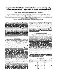
5.1.1 Repetitive controller In its basic layout, the repetitive controller M consists of a delay of length T0 = 2π/ω0 and positive feedback. The positive feedback in the memory loop generates infinite gain at the harmonics of the operating frequency. The time period of this operating frequency is equal to the total internal delay in the memory loop. In Fig. 6 a block diagram of the applied repetitive controller is shown. The controller consists of two delays, a robustness filter Q(z), constant gain blocks γ, γ −1 , DC reconstruction filter DC(z) and learning filter L(z). The delays are implemented as discrete time FIFO shift registers. Their total length is N − q − l and l respectively with N = T0 · fs , fs being the sampling frequency of the memory loop. The constants q and l are the delays caused by the linear phase lowpass filter Q(z) and the learning filter L(z) required for stability. The DC reconstruction filter is required for canceling the gain at 0Hz in the memory loop. Without this filter, the DC amplification in the memory loop will be infinite so there will be no feedback at 0Hz in a repetitive control system. This is undesirable in applications where DC feedback is required for the system to function like for example positioning systems subjected to gravity. The output of the DC reconstruction filter, which equals the DC level of the memory loop, is subtracted from the memory loop signal (Fig. 6). The transfer function of the DC reconstruction filter is given by the following comb-filter: DC(z) =

1 z N −1 + z N −2 + ... + z 0 N N z

(8)

The upper trace of Fig. 7 shows the magnitude of the Frequency Respons Function (FRF) of the ideal memory loop without DC reconstruction. The FRF of the memory loop with DC reconstruction filter is shown in the lower trace of Fig. 7. +

z-(N-q-l)

Ó

Q(z) +

+

ã z-l

L(z)

Ó ã-1

-

DC(z)

Figure 6: Memory loop with positive feedback and DC reconstruction filter.

Mag [dB]

400 200 0 −200 0

2

4 6 Harmonic number

8

10

2

4 6 Harmonic number

8

10

Mag [dB]

400 200 0 −200 0

Figure 7: Magnitude of the FRF of the memory loop, without (upper trace) and with DC reconstruction filter (lower trace).

5.1.2 Stability In order to successfully apply the memory loop as an add-on device under measurement conditions, overall system stability must be preserved [28, 29, 30]. The transfer function of the memory loop M is given by: M (z) =

Qz −(N −q−l) (1 − DC)L 1 − Qγz −(N −q)

(9)

Assuming linearity of H, Eq. 7 can be rewritten as: T =−

CH CH =− Ms 1 + CH + M 1 + CH

(10)

Ms is the modifying complementary sensitivity function and describes the modification of the complementary sensitivity function of the original system without repetitive control. Substituting Eq. 9 in Eq. 10 yields: Ms (z) =

1 − Qγz −(N −q) 1 − Qz −(N −q) {γ − SLz l (1 − DC)}

(11)

where S is the sensitivity:

1 1 + CH From Eq. 11 a sufficient condition for stability based upon small gain assumptions can be derived: S=

|Qz −(N −q) {γ − SLz l (1 − DC)}| < 1

(12)

(13)

for all z with |z| = 1. Since |Q| ≤ 1, the stability criterion (Eq. 13) can be reduced to |γ − SLz l (1 − DC)| < 1

(14)

At 0Hz |1 − DC| = 1, for all other frequencies |1 − DC| < 1. So stability is guaranteed if |γ| = 1 − ǫ and L = S −1 . The learning filter L can be designed with the ZPETC algorithm [31] and the resulting phase delay of l samples is absorbed in the two delay blocks. Depending upon the characteristics of S, an additional notch-filter may be required to reduce the DC gain of the L filter in order to maintain DC feedback in the main system. The notch should not be positioned inside the memory loop since it does not exhibit a linear phase characteristic like the robustness filter Q. As a result its delay can not be compensated resulting in a significant reduction of the gain at the harmonics of the excitation frequency. Since the gain block γ does not exhibit phase shift, its influence on the memory loop gain is significantly less.

5.2 Signal processing The Fast Fourier Transform (FFT) will be applied for the transformation of the time-domain data into frequency-domain information. This transformation guarantees infinite selectivity for harmonically related signals if the record length Tb is chosen correctly with respect to the signals to be analyzed. Both the input signal u(t) and output signal y(t), (Fig. 1) are Fourier transformed with a transform size of 2m. The resulting single sided spectra contain m + 1 frequency lines each with 0Hz in frequency line zero. The frequency spacing is ∆f = 1/Tb with Tb the length of the data block. Tb is chosen a multiple p times the period T = 2π/ω of the output signal y(t). This assures that all the power of the output signal is concentrated in frequency-line p. The power of the excitation signal u(t) is fully concentrated in the frequency lines n.p with n ∈ N, so leakage is absent. In Fig. 8 the filter bank, the Virtual Harmonics Compressor and the kth order HOSODF are highlighted. Let us consider the calculation of the kth order HOSODF. According to Eq. 6 this HOSODF is calculated from the kth harmonic component y˘k (t) of the VHC of the system divided by the kth harmonic component u ˘k (t) of the input signal u(t). The signal y˘k (t) however cannot be measured but has to be derived from the measurable output signal y(t). Using Eq.1, 2 the frequency nω, amplitude a ˆ and phase

¥

å A (aˆ,w) cos(n(wt + j) + j (aˆ,w)) = n

n

n=0

u(t )

R0(â,ω)

0

. . .

Filter bank

FFT

k

Rk(â,ω) . .

n

Rn(â,ω)

Virtual Harmonics Compressor

y (t ) = aˆ cos(wt + j )

FFT

( uk (t ) = Ak (aˆ , w ) cos(k (wt + j )) = Ak (aˆ , w ) cos(kwt + j k ) in

kp w akp, bkp

( yk (t ) = aˆ cos(k (wt + j )) = aˆ cos(kwt + j k )

akp2 + bkp2 = Ak (aˆ , w ) tan(j k ) = in

out

- bkp

a 2p + b p2 = aˆ tan(j ) =

akp

w

p a p, b p

- bp ap

Figure 8: Determination of the kth order HOSODF. nϕ of every component n at the input of the VHC can be calculated. In the spectrum of y(t), the frequency line with number p and complex value ap + jbp represents the output signal. The square root of the power in this frequency line is the amplitude a ˆ: q a ˆ=

a2p + b2p

(15)

The phase angle of this frequency line equals: −bp ap ) −bp arctan( ap ) +

ϕ = arctan( ϕ=

π

if

ap ≥ 0

if

ap < 0

(16)

In the frequency spectrum of u(t) the frequency line k · p with complex value akp + jbkp represents the harmonic component under consideration of the input signal. The square root of the power in this frequency line is the amplitude Ak (ˆ a, ω) and the phase angle of this frequency line equals phase ϕkin : q (17) Ak (ˆ a, ω) = a2kp + b2kp −bkp akp ) −bkp arctan( akp ) + π

ϕkin = arctan(

if

akp ≥ 0

ϕkin =

if

akp < 0

(18)

with ϕkin = kϕ + ϕk (ˆ a, ω) From Eq. 15, 17 the magnitude of the

(19)

kth

order HOSODF can be calculated as: q a2p + b2p |Rk (ˆ a, ω)| = q a2kp + b2kp

(20)

The phase ϕk (ˆ a, ω) of the kth order HOSODF can be calculated from Eq. 16, 18, 19: −bkp −bp ap )]mod2π − arctan( akp ) −b −b [k{arctan( app ) + π}]mod2π − arctan( akpkp ) −b −b [k arctan( app )]mod2π − arctan( akpkp ) − π −b −b [k{arctan( app ) + π}]mod2π − arctan( akpkp ) − π

ϕk (ˆ a, ω) = [k arctan( = = =

if

ap ≥ 0, akp ≥ 0

if

ap < 0, akp ≥ 0

if

ap ≥ 0, akp < 0

if

ap < 0, akp < 0

(21)

6 Conclusion and future work A new description of the dynamic behavior of a specific class of non-linear systems was presented. It was shown that causal, stable, time-invariant systems with a sinusoidal response to a harmonic excitation can be modeled as a parallel connection of non-linear subsystems in series with a Virtual Harmonics Compressor. The dynamic behavior of these non-linear subsystems was described with the Higher Order Sinusoidal Output Describing Functions (HOSODF), a generalization of the theory of the Describing Functions. A repetitive control loop consisting of a digital memory loop with positive feedback was proposed in order to force the output of the non-linear system to be sinusoidal. A stability analysis of the learning filter based on small gain assumptions resulted in a sufficient condition for stability. A practical methode for the non-parametric identification of Higher Order Sinusoidal Output Describing Functions was presented. This method was based on the Fast Fourier Transform and allows leakage free measurements. The proposed method of using repetitive control for the nonparametric identification of HOSODF possibly has an interesting mechanical application. In particular mechanical testing situations, like normal mode testing [32], a sinusoidal excitation force is required. Conventional sine testing instrumentation employs linear feedback techniques to compensate for the influence of the linear dynamics of the system under test on the shaker system. The actual shaker force signal is fed back to a controller which is implemented as a linearized, inverse model of the system under test. This allows the magnitude of the required excitation frequency component to be controlled. However, the true system under test is non-linear, and its non-linear mechanical impedance will force the sinusoidal excitation signal to become harmonic. By employing the HOSODF approach, a data-based inverse representation of the non-linear system H is incorporated in the control loop. If the shaker force is considered the output y(t) of a non-linear system H (Fig. 5), implementing the repetitive control loop M will result in a sinusoidal output of the shaker if the non-linear system H belongs to class O . Future work will concentrate on designing a calibration experiment from which the learning filter can be determined automatically. An additional research question is the investigation of the properties a non-linear system must have in order to belong to the class O .

References [1] C. Evans and D. Rees. Non-linear distortions and multisine signals - part ii: Minimizing the distortion. IEEE Transactions on Instrumentation and Measurement, 49(3):610–616, June 2000. [2] R. Pintelon and J. Schoukens. System Identification: A Frequency Domain Approach. John Wiley&Sons Inc, 2001. [3] M. Solomou, C. Evans, and D. Rees. Crest factor minimisation in the frequeny domain. In Conference Proceedings of the IEEE Instrumentation and Measurement Technology Conference, pages 1375–1381, Budapest, Hungary, May 2001. [4] J. Schoukens, T. Dobrowiecki, and R. Pintelon. Parametric and nonparametric identification of linear systems in the presence of non-linear distortions- a frequency domain approach. IEEE Transactions on Automatic Control, 43:176–190, 1998.

[5] C. Evans and D. Rees. Non-linear distortions and multisine signals - part i: Measuring the best linear approximation. IEEE Transactions on Instrumentation and Measurement, 49(3):602–609, June 2000. [6] M. Solomou, D. Rees, and N. Chiras. Frequency domain analysis of non-linear systems driven by multiharmonic signals. IEEE Transactions Instrum. Meas., 53:243–250, 2004. [7] J. Schoukens, R. Pintelon, T. Dobrowiecki, and Y. Rolain. Identification of linear systems with nonlinear distortions. Automatica, 41:491–504, 2005. [8] S. Boyd and L.O. Chua. Fading memory and the problem of approximating non-linear operators with volterra series. IEEE Transactions on Circuits and Systems, CAS-32(11):1150–1161, Nov. 1985. [9] V. Volterra. Theory of functionals and of integral and integro-differential equations. S.I., Dover, 1959. Reprint from the 1931 Macmillan edition. [10] M. Schetzen. The Volterra and Wiener Theories of Non-linear Systems. John Wiley, Chichester, 1980. [11] W.J. Rugh. Non-linear System Theory: the Volterra/Wiener Approach. Johns Hopkins University Press, Baltimore, Maryland, USA, 1981. [12] D.A. George. Continuous non-linear systems. Technical Report 355, MIT Research Laboratory of Electronics, Cambridge, Mass., July 1959. [13] E. Bedrosian and S.O. Rice. The output properties of volterra systems (non-linear systems with memory) driven by harmonic and gaussian inputs. In Proceedings IEEE, volume 59, pages 1688–1707, 1971. [14] S. Boyd, Y.S. Tang, and L.O. Chua. Measuring volterra kernels. IEEE Transactions Circuits Syst., CAS-30-8:571–577, 1983. [15] L. Chua and Y. Liao. Measuring volterra kernels (ii). International J. of Circuit Theory and Applications, 17:151–190, 1989. [16] S.A. Billings and K.M. Tsang. Spectral analysis for non-linear systems, part1: Parametric non-linear spectral analysis. Mechanical Systems and Signal Processing, 3(4):319–339, 1989. [17] J.C. Peyton Jones and S.A. Billings. Interpretation of non-linear frequency response functions. International J. Control, 52(2):319–346, 1990. [18] R. Yue, S.A. Billings, and Z.Q Lang. An inverstigation into the characteristics of non-linear frequency response functions. part 1: Understanding the higher dimensional frequency spaces. International Journal of Control, 78(13):1031–1044, 2005. [19] A. Gelb and W.E. Vander Velde. Multiple input describing functions and non-linear system design. McGraw Hill, New York, 1968. [20] J. Taylor. Electrical Engineering Encyclopedia: Describing Functions. John Wiley & Sons Inc., New York, 1999. [21] P.W. Nuij, O.H. Bosgra, and M. Steinbuch. Higher-order sinusoidal input describing functions for the analysis of non-linear systems with harmonic responses. Mechanical Systems and Signal Processing, 20(8):1883–1904, 2006. [22] P.W.J.M. Nuij, M. Steinbuch, and O.H. Bosgra. Experimental characterization of the stick/slip transition in a precision mechancal system using the third order sinusoidal input describing function. Mechatronics, 18(2):100–110, 2007.

[23] P.W.J.M. Nuij, M. Steinbuch, and O.H. Bosgra. Measuring the higher order sinusoidal input describing functions of a non-linear plant oprating in feedback. Control Engineering Practice, 16(1):101–113, 2007. [24] S.A. Billings and K.M. Tsang. Spectral analysis for non-linear systems, part ii: interpretation of nonlinear frequency response functions. Mechanical Systems and System Processing, 3(4):341–359, 1989. [25] M. Solomou, C. Evans, D. Rees, and N. Chiras. Frequency domain analysis of non-linear systems driven by multiharmonic signals. In IEEE Instr. and Meas. Techn. Conf. Anchorage, pages 799–804, 2002. [26] K. Narendra and P. Gallman. An iterative method for the identification of non-linear systems using a hammerstein model. IEEE Transactions Automat. Control, 11:546–550, 1966. [27] M. Steinbuch. Repetitive control for systems with uncertain period-time. Automatica, 38(12):2103– 2109, 2002. [28] M. Tomizuka, T.C. Tsao, and K.K. Chew. Discrete-time domain analysis and synthesis of repetitive controllers. In Proc. 1988 American Control Conference, pages 860–866, 1988. [29] G. Hillerstr¨om. Adaptive suppression of vibrations–a repetitive control approach. IEEE Transactions on Control Systems Technology, 4(1):72–77, 1996. [30] K.K. Chew and M. Tomizuka. Digital control of repetitive errors in disk drive systems. In Proceedings of the American Control Conference, pages 540–548, 1990. [31] M. Tomizuka. Zero phase error tracking algorithm for digital control. Journal of dynamic systems, measurement and control, 109:65–68, 1987. [32] B.S. Gabri and J.T. Matthews. Normal mode testing using multiple exciters under digital control. Journal of the Society of Environmental Engineers, 19(1):25–34, 1980.