International Journal of Robotics and Automation, Vol. 17, No. 2, 2002
NONCOMMENSURATE SYSTEMS IN ROBOTICS E. Schwartz,∗ R. Manseur,∗∗ and K. Doty∗∗∗
Abstract
to interaction between physical units is necessary in any control system. Other examples of mishandling of physical units in the mathematical development of systems in the area of robot manipulator control are given below. This article also discusses the physical inconsistency of some noncommensurate systems and presents results and techniques for ensuring that mathematical developments involving noncommensurate systems are physically consistent. One type of noncommensurate systems familiar to the authors is the control of robot manipulators where position with units of distance combines with orientation with units of angle, and prismatic mechanical joints and revolute joints are parts of the same robotic structure. The theory of hybrid control of robot manipulators developed by Mason in 1978 [3] and further expanded by Raibert in 1981 [4] has been shown to introduce inconsistencies [5–8]. Although the aim of hybrid control is to produce an optimal solution based on some optimality criterion, the end result is a solution that is nonoptimal with respect to any fixed criteria and is in fact quite arbitrary. One major problem is due to the assumption and use of orthogonality in vector spaces with vectors that include elements of different physical nature. Such nonhomogeneous vectors do not have a physically consistent Euclidian norm. The robotics literature [9–14] uses mathematical developments based on the eigenvalues, eigenvectors, or singular values of matrices that represent robotic systems with physical quantities of different nature. The results of this article indicate the invalidity, in terms of physical consistency, of such mathematical developments. In particular, it is shown that systems that combine different physical units have inconsistent eigenvalues, eigenvectors, and singular values. Robot manipulability theory, based on the product of the manipulator Jacobian and its transpose (JJ T ) has now taken hold within a robotics research community largely unaware of the physical inconsistency and the arbitrary nature of this theory in the case of noncommensurate systems [16–19]. Advanced robotics textbooks teach and discuss manipulator manipulability, manipulability ellipsoids, manipulability indexes, and their applications without discussing the arbitrary nature of such control measures [20, 21]. This article clearly establishes the arbitrariness and physical inconsistency of manipulability measures based
In certain areas of science and technology, physical quantities of different natures are combined in a variety of involved mathematical processes that obscure the interaction of these physical units and sometimes lead to unreliable results. Noncommensurate systems are those in which either the input vector or the output vector contains elements with different physical units. An example is the control of robot manipulators where position with units of distance and orientation with units of angle must be combined. Unless proper care is taken, control systems based on current optimization techniques may yield inaccurate and misleading results. This article examines properties of noncommensurate systems and develops several algebraic properties and requirements for the physical units involved in the control methods for such systems.
Key Words Noncommensurate, units, robotics, control
1. Introduction Control systems that combine physical quantities with different units present an additional challenge over those that concern quantities with similar physical units. Recent developments in control theory have shown that certain mathematical techniques based on eigensystems, singular value decomposition, and pseudo-inverses may lead to inconsistent and erroneous results [1, 2]. Although the rules for combining physical quantities of different units are considered largely trivial, many recent advances and mathematical processes have become complex enough to obscure the interaction of variables of different units, and in some cases have led researchers astray. The unfortunate loss of the Mars Climate Observer spacecraft in September 1999 was officially blamed on a mismatch of units between two separate research centres by the National Aeronautical and Space Agency (NASA). This incident comes as a costly reminder of the importance of the physical units in system analysis and development and shows that, although considered by many as a trivial exercise, careful attention ∗
Machine Intelligence Laboratory, Electrical and Computer Engineering, University of Florida, Gainesville, FL 32611-6200, USA ∗∗ Robotics and Image Analysis Lab, Electrical and Computer Engineering, University of West Florida, Gainesville, FL 326116200, USA; e-mail:
[email protected] ∗∗∗ Mekatronix Corporation, 316 NW 17 Street, Suite A, Gainesville, FL 32603, USA (paper no. 206-2014)
1
on JJ T and also proposes rules and guidelines for the mathematical manipulations required to maintain physical consistency in nonhomogeneous systems. Noncommensurate systems are introduced and formally defined in this work. It is shown that eigenvalues and vectors and singular values of noncommensurate systems are not physically consistent, as they require addition of quantities of different units. Tests for physical consistency of a system are established and presented. In robotics in particular, the manipulator Jacobian, a central analysis and control tool, is examined in light of the physical units attached to its elements, and the consequences of using the Jacobian in robot control and manipulability studies are discussed. For ease of reference, we start with a definition of noncommensurate systems.
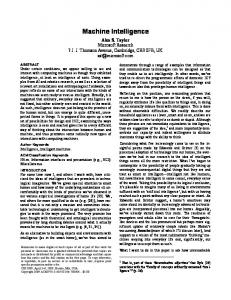
proper choice of units for the elements of the system matrix J. To illustrate this point, consider the following example. Example 1. The robot manipulator defined by the Denavit-Hartenberg parameters [15] in Table 1 and described in Fig. 1 is redundant if only position is considered in the task space. Table 1 DH Parameters Joint d
2. Noncommensurate Systems We define noncommensurate systems as those involving physical quantities with different units that are nonetheless described and controlled by physically consistent equations. Physical consistency refers here to the physical validity of all system equations in the sense of combining quantities of different units in a meaningful way. Empirically, it is about making sure that "oranges are added to oranges" and avoiding adding "apples to oranges." In general, systems fall within one of three broad categories: 1. Commensurate systems: These are systems that involve only quantities of similar units, whereby the input vector elements as well as the output vector elements are all expressed in the same physical unit. Ensuring physical consistency in these systems is trivial since a single unit is involved. 2. Noncommensurate systems: These are the topic of interest of this work. They involve different physical quantities and therefore combine different units in a physically consistent way. It is important to understand that we include in this category only those systems with mixed physical units but with equations that are all physically consistent 3. Non-physically consistent systems: Systems that have vectors with mixed units and are modelled by equations that are physically inconsistent. In other words, the equations that describe the system violate the "apples added to apples" rule. Non-physically consistent systems arise from mathematical developments that inadvertently and incorrectly combine different units and are, in general, not intended. As a simple example of a noncommensurate system, the velocity vector V of the end-effector of a robot manipulator is related to the joint rates vector q by the manipulator Jacobian matrix J in the linear equation V = J q. ˙ The velocity vector, also known as the twist, V = [v, ω]T , is composed of the linear velocity vector v, with units of distance/time, and the angular velocity vector ω, with units of angle/time. Vector q˙ may have elements of angular velocity for revolute joints and elements of linear velocity for prismatic joints. Physical consistency is achieved by
a
α
θ
1
0 a1 0 θ1
2
d2 0 90 0
3
0 a3 90 θ3
4
0 a4 0 θ4
Figure 1. Redundant robot.
Forward kinematics computations yield the endeffector position vector: px p = py = pz
a4 (c1 c3 c4 + s1 s4 ) + a3 c1 c3 + a1 c1 a4 (s1 c3 c4 − c1 s4 ) + a3 s1 c3 + a1 s1 a4 s3 c4 + a3 s3 + d2
where we used the customary notation ci = cos(θi ) and si = sin(θi ). As position is determined by a minimum of three degrees of freedom, the robot under consideration, with its four joints, is redundant with respect to position. This robot is chosen because it contains prismatic and rotational joints. The velocity vector of the end-effector frame is given dpz T x dpy ˙ ˙ ˙ ˙ T by v = J q˙ where v = dp dt , dt , dt , q˙ = [θ1 d2 θ3 θ4 ] is the joint velocity vector and J is the Jacobian matrix of the robot. The Jacobian matrix is expressed as:
insert Matrix as figure.
In terms of units, all elements of matrix J have units of length except for the second column, whose elements are unitless numbers. This makes (1) physically consistent, as all elements of vector q˙ are in units of inverse time (time−1 ) except for the second element, which has units of velocity (length/time). Manipulability studies rely on the product JJ T , whose elements are listed here: T JJ11 = (−s1 (c3 a4 c4 +a3 c3 )+c1 a4 s4 −a1 s1 )2 +c21 (−s3 a4 c4 − a3 s3 )2 + (−c1 c3 s4 + s1 c4 )2 a24 T JJ12 = (−s1 (c3 a4 c4 + a3 c3 ) + c1 a4 s4 − a1 s1 )(c1 (c3 a4 c4 + a3 c3 ) + s1 a4 s4 + a1 c1 ) + c1 (−s3 a4 c4 − a3 s3 )2 s1 + (−c1 c3 s4 + s1 c4 )(−s1 c3 s4 − c1 c4 )a24
2
T JJ12 = c1 (−s3 a4 c4 − a3 s3 )(c3 a4 c4 + a3 c3 ) − (−c1 c3 s4 + s1 c4 )s3 s4 a24 T JJ21 = (−s1 (c3 a4 c4 + a3 c3 ) + c1 a4 s4 − a1 s1 )(c1 (c3 a4 c4 + a3 c3 ) + a1 a4 s4 + a1 c1 ) + c1 (−s3 a4 c4 − a3 s3 )2 a1 + (−c1 c3 s4 + s1 c4 )(−s1 c3 s4 − c1 c4 )a24 T JJ22 = (c1 (c3 a4 c4 +a3 c3 )+s1 a4 s4 +a1 c1 )2 +s21 (−s3 a4 c4 − a3 s3 )2 + (−s1 c3 s4 − c1 c4 )2 a24 T JJ23 = s1 (−s3 a4 c4 − a3 s3 )(c3 a4 c4 + a3 c3 ) − (−s1 c3 s4 − c1 c4 )s3 s4 a24 T JJ31 = c1 (−s3 a4 c4 − a3 s3 )(c3 a4 c4 + a3 c3 ) − (−c1 c3 s4 + s3 s4 a24 T JJ32 = s1 (−s3 a4 c4 − a3 s3 )(c3 a4 c4 + a3 c3 ) − (−s1 c3 s4 − c1 c4 )s3 s4 a24 T JJ33 = 1 + (c3 a4 c4 + a3 c3 )2 + s23 a24 s24
yi =
aij xj
(2)
j=1
For consistency, we require that: units(yi ) = units(aij ) units(xj )
(3)
for all i, j. Using two distinct terms of the sum (2), for two elements of y, we get:
Careful examination of the units involved in the above equations indicates that each element of JJ T is actually the sum of a quantity of length-squared added to a unitless quantity. The unitless quantity is 0 in all elements of JJ T T except in JJ33 , where it is equal to 1. This example shows that the matrix JJ T does not make physical sense and represents a non-physically consistent system. The determinant of JJ T (or its square root) is typically used as a measure of manipulability at the current robot configuration. Choosing rotational joint values of θ1 = π π π 6 , θ3 = 6 , and θ4 = − 6 rather arbitrarily and computing the determinant of the matrix JJ T defined above yields:
zi = aij xj + aik xk
(4)
zl = aij xj + alk xk
(5)
for all i, j, k, l, where units(zi ) = units(yi ). Manipulating equations (4) and (5) yields: aik zl − alk zi = (aik alj − aij alk )xj
(6)
Physical consistency demands that: units(aik ) units(alj ) = units(aij ) units(alk )
(7)
alk aik ] = units[ ], for aij 6= 0 and alj 6= 0 aij alj
(8)
or:
d= 1.125 a4 a1 a23 +.6495a4 a33 +.75a34 a23 a1 +.3248a34 a33 + .7307a34 a3 + .25a21 a23 a24 + .433a33 a1 + .1406a44 a23 + .1875a24 a43 + 1.172a24 a23 + .375a24 a21 + .1875a43 + .25a21 a23 + .2578a44 + .433a33 a1 a24 + .4330a21 a34 a3 + .3248a44 a3 a1 +.1875a34 a1 +1.299a24 a1 a3 +.4330a21 a4 a3
units[
In other words, if m-2 columns and n-2 rows are eliminated, the determinant of the remaining 2x2 matrix must be physically consistent for the system to be noncommensurate. This result is summarized in a theorem as a verification test for the commensurate or noncommensurate nature of a matrix A. Theorem 1. The linear equation y = Ax, where x and/or y are noncommensurate vectors, describes a noncommensurate system if and only if the determinant of any 2x2 matrix obtained by eliminating all but two rows and all but two columns of A is physically consistent. Using three terms from the sum (2) for three elements of vector y, we get three equations of the form of (4) and (5). Manipulating these three equations leads to the result that physical consistency requires that the determinant of any 3x3 matrix obtained by the elimination of m-3 rows and n-3 columns be physically consistent for the system to be noncommensurate. By induction, we provide that a condition for the system of (1) to be noncommensurate is that the determinant of any ixi matrix obtained by eliminating (m − i) rows and (n − i) columns must be physically consistent. Another requirement may be obtained by partially expanding (1) as follows:
as the determinant. Again, examination of the units involved shows that d is not physically consistent, as terms of units length-to-the-sixth-power are added to terms with units of length-to-the-fourth-power. Manipulability theory applied to redundant robots does not lead to consistent results, as shown in this example. The goal of this article is to examine the problems associated with systems involving physical quantities of different units and establish a few ground rules for such systems. 3. Linear Noncommensurate Systems A vector of elements of unlike physical units is defined as a noncommensurate vector, also known as a compound or nonhomogenous vector. A linear system is described by a linear equation of the form: y = Ax
m X
(1)
where x = [x1 , x2 , . . . , xn ]T and y = [y1 , y2 , . . . , ym ]T are vectors and A = {aij }i=1,...,n;j=1,...,m is an n × m matrix. Let us assume that x and y in (1) are noncommensurate vectors. In this section we will determine conditions on the coefficient matrix A for the system (1) to be physically consistent. The ith component of vector y is given by:
u1 m X .. = .
a1j .. . xj
un
anj
j=1
3
(9)
It follows that the units of any two columns of A must be proportional for consistency. This is another expression of the result of (8) and a simple way to visually evaluate the possible noncommensurate nature of matrix A. Corollary 1.1. A matrix A, with elements of different units, is noncommensurate if and only if the units of any two columns of the matrix are proportional. Note that in the case of commensurate matrices, all elements have the same unit; therefore Corollary 1.1 essentially indicates that a matrix A, whose columns have proportional units, will lead to a physically consistent system described by (1).
5. Singular Value Decomposition Many processes in system control rely on a singular value decomposition. In this section, the physical consistency of singular values in noncommensurate systems is examined. The singular values of matrix A are the non-negative square roots of the non-zero eigenvalues of the square matrices AAT and AT A. A test similar to those discussed above on these matrix products will determine if the SVD of matrix A is physically consistent. Let B = AAT or B = AT A and x and λ be an eigenvector and eigenvalue of B, respectively. From Theorem 1 above, physical consistency requires that:
4. Eigenvalues in Noncommensurate Systems units[bkj ] units[xj ] = units[λ] units[xk ] The treatment of (1) in many applied fields requires computation and use of eigenvalues and eigenvectors. In this section, the physical consistency of eigenvalues and eigenvectors is examined and conditions on the coefficient matrix A are established for physical consistency. Let e be an eigenvector of matrix A, and λ the corresponding eigenvalue; then:
where B = biji=row index, j=column index . For diagonal elements of B, (12) yields units[bkk ] = units[λ], which indicates that all diagonal elements of B must have the same units. If A is an n × m matrix, then the diagonal elements of B are given by: Pm
a11 a12 . . . a1n e1 a21 a22 . . . a2n Ae = . .. .. .. .. . . .
e2 .. = λe .
bkk = Pj=1 n
a2kj , for B = AAT
2 T j=1 ajk , for B = A A
(10)
for all k
(13)
Therefore, all the elements in the kth row (for B = AAT ) or the kth column (for B = AT A) must have identical units. As all diagonal elements must also have the same units, the singular value decomposition is physically consistent only for commensurate systems. Theorem 3: Noncommensurate systems do not have a physically consistent singular value decomposition. Theorem 3 indicates that any development based on the singular value decomposition of a matrix with different units is invalid in the sense of physical consistency. Example 2: The field of robotics offers an example of the invalid use of the eigensystem and SVD. Consider a redundant robot manipulator described by the DH parameters of Table 2. This robot has three positional prismatic joints and a four-joint wrist. The Jacobian matrix J for this robot is not square, and the pseudo inverse is typically used in solving kinematic equations. The matrix JJ T is used in the computation of the pseudoinverse of J, [Ben-Israel 1974] and a manipulability measure is defined by:
an1 an2 . . . ann en Expanding: a11 e1 + a12 e2 + · · · + a1n en = λe1 a21 e1 + a22 e2 + · · · + a2n en = λe2 .. .
(12)
(11)
an1 e1 + an2 e2 + · · · + ann en = λen As meaningful addition must be with terms of identical units, the following theorem on the units involved must hold. Theorem 2: The equation Ax = λx is physically consistent if and only if: units[akj ] units[xj ] = units[xk ] for all j and k Direct consequences of this theorem are: Corollary 2.1: The equation Ax = λx is physically consistent only if units[λ] = units[aii ] for all i. Corollary 2.2: The equation Ax = λx is physically consistent if and only if units[akj ]units[ajk ] = units[a2ii ] for all i, j, and k. From Corollary 2.1, any matrix A with a physically consistent eigenvalue equation must have diagonal elements with the same physical units and all its eigenvalues must have those same units.
ρ=
q det(JJ T )
(14)
Further, Yoshikawa [14] and others [11, 12] define a manipulability ellipsoid with principal axes in the direcT tions of the given a p eigenvectors of JJ . Each axis is length of 1/λi where λi is an eigenvalue of JJ T . Table 2 DH Parameters for a 3P-4R Robot 4
Joint Type d a
θ
α
0
π/2
1
P
d1 0
2
P
d2 0 π/2 π/2
3
P
d3 0
4
R
0 0 θ4 π/2
5
R
0 0 θ5 π/2
6
R
0 0 θ6 π/2
7
r
0 0 θ7
0
shown in Figure 2 in a configuration where θ1 = 120◦ , θ2 = −75◦ , and d3 = 0.04.
Figure 2. Redundant planar robot.
0
Table 3 Joint d
0
For an all-revolute manipulator, the matrix JJ T is a 6x6 matrix that is physically consistent and can be viewed as formed with 3x3 block matrices B11 , B12 , B21 , and B22 , that is:
JJ T =
B11 B12
a
α
θ
0
θ1 rotational
Note
1
0 0.1
2
0 0.1 90◦ θ2 rotational
3
d3
0
0
0 prismatic
This robot is redundant if the end-effector position is the only task requirement. The position is readily computed as:
(15)
a2 c1 2 + d3 s12 + a1 c1 x p= = a2 s12 − d3 c1 2 + a1 s1 y
B21 B22 Each block matrix has its own physical units. For an allrevolute robot arm, B11 has elements with units of lengthsquared (length2 ), B12 and B21 have units of length, and B22 is unitless. Let L stand for units of length and U for unitless. Then the units of the main diagonal of JJ T are represented by [L2 , L2 , L2 , U, U, U ]. As the units of the elements of the main diagonal are not all the same, Corollary 1 of Theorem 1 above states that JJ T does not support a physically consistent eigensystem. This invalidates any development based on the eigensystem of the matrix JJ T . If the manipulator is not all revolute, then the JJ T matrix is itself physically inconsistent because B11 , defined in (15), has units of [L2 + U ]. Example 1 discussed above supports this discussion.
The manipulator Jacobian is:
J =
−a2 s12 + d3 c12 − a1 s1 − a2 s12 + d3 c12 s12
a2 c12 + d3 s12 + a1 c1 a2 c12 + d3 s12 − c12
Note that the first two columns of J have units of distance whereas the third column has no units. Fig. 3 shows two manipulability ellipsoids. The ellipse on the left is obtained if the structure of the robot is described using meters (i.e., a1 = a2 = 0.1 m and d3 = 0.0707 m). The ellipse on the right results from using centimeters as the units of length (i.e., a1 = a2 = 10 cm, and d3 = 7.07 cm). In this experiment, the rotational joints values are θ1 = π/4, θ2 = -π/4 which locates the end-effector close to the x-axis.
6. Robot Manipulability The possibility of circumventing the inherent physical inconsistencies of the manipulator Jacobian by use of weight matrices is discussed in [8], and application to robot manipulability is developed in [10]. The use of unit-adjusting weights on the vectors and matrices of a system to eliminate the inconsistencies caused by different units is established, but all results derived from manipulability ellipsoids such as direction of axes and their lengths become dependent, not only on the robot structure and configuration, but also on the chosen weights. Therefore, all manipulability studies and results should be specified as valid not only for the current robot configuration and the unit-adjusting weights but also for the physical units used to describe the robot structure. A simple example proves this point. Example 3: A robot manipulator described in Example 1.1 in [2] is used here to illustrate the arbitrary nature of manipulability measures in the case of redundant manipulators with mixed rotational and translational joints. The DH parameters of this robot are given in Table 3 and
Figure 3. Manipulability ellipsoids.
It is quite clear that the ellipses are very different and measures derived from them will be equally different, yet the robot is the same and so is the configuration. The only difference is the (rather arbitrary) choice of units of length. Others using inches or feet will get different results as well. The same ellipses will be obtained assuming that the units have all been adjusted by using unity weights. As discussed in [10], the choice of unit adjusting weights only adds another level of arbitrariness to the manipulability ellipsoids. 7. Conclusion This article has addressed the problem of noncommensurate systems from the point of view of physical consistency. 5
An analysis of the units involved in the mathematical derivations routinely performed in the control of noncommensurate systems provides a few tests for physical consistency that can be readily applied to linear hybrid systems where physical quantities of different nature are combined in the controls equations. In particular, the use of eigenvalues, eigenvectors, and singular values in the control of noncommensurate systems is shown to lead to physically inconsistent results. This work uses examples in robotics to illustrate the concepts discussed and presented, but the results apply to any control algorithm based on equations derived through the use of eigenvalues, eigenvectors, or singular values of matrices whose elements have different units.
[19] J. Kovecses, R.J. Fenton, & W.L. Cleghorn, Effects of joint dynamics of the geared robot manipulators, Mechatronics 11, 2001, 43–58. [20] Y. Nakamura, Advanced robotics, redundancy and optimization (New York: Addison-Wesley, 1991). [21] L. Sciavicco & B. Siciliano, Modeling and control of robot manipulators (New York: McGraw-Hill, 1996).
References [1] E.M. Schwartz & K.L. Doty, The weighted generalized-inverse applied to mechanism controllability, Sixth Annual Conference on Recent Advances in Robotics, Gainesville, FL, 1993. [2] E.M. Schwartz, Algebraic properties of noncommensurate systems and their applications in robotics, doctoral diss., University of Florida, Gainesville, FL, 1995. [3] M.T. Mason, Compliance and force control for computer controlled manipulators, master’s thesis, Massachusetts Institute of Technology, Cambridge, MA, 1978. [4] Nf. H. Raibert. & J.J. Craig, Hybrid position/force control of manipulators, ASME. Dynamic Sys. Aleas. Contr., 102, 1981, 126–133. [5] H. Lipkin & J. Duffy, The elliptic polarity of screws, ASME Journal of Mechanisms, Transmissions, and Automation in Design, 107, 1985, 377–387. [6] H. Lipkin & J. Duffy, Hybrid twist and wrench control for a robotic manipulator, ASME Journal of Mechanisms, Transmissions, and Automation in Design, 110, 1988, 13 144. [7] A. Abbati-Marescotti, C. Bonivento, & C. Melchiorri, On the invariance of the hybrid position/force control, J. Intelligent and Robotic Systems, 3, 1990, 23 250. [8] K.L. Doty, C. Melchiorri, & C. Bonivento, A theory of generalized inverses applied to robotics, Int. J. Robotics Research, 12(1), 1993, 1–19. [9] P. Chiacchio, S. Chiaverini, L. Sciavicco, & B. Siciliano, Global task space manipulability ellipsoids for multiple-arm systems, IEEE J. Robotics and Automation, (5), 1991, 678–684. [10] K.L. Doty, C. Melchiorri, E.M. Schwartz, & C. Bonivento, Robot manipulability, IEEE Trans. on Robotics and Automation, 11(3), 1995, 462–468. [11] C.A. Klein & B.E. Blaho, Dexterity measures for the design and control of kinematically redundant manipulators, Int. J. Robotics Research, 6(2), 1987, 72–82. [12] Y.C. Park & G.P. Starr, Optimal grasping using a multifingered robot hand, IEEE Conf. on Robotics and Automation, Cincinnati, OH, 1990, 689–694. [13] C.W. Wangler II, Manipulator inverse kinematic solutions based on vector formulations and damped least-squares methods, IEEE Trans. on Systems, Man, and Cybernetics, SMC16(1), 1986, 9 101. [14] T. Yoshikawa, Manipulability of robotic mechanisms, Int. J. of Robotics Research, 4(2), 1985, 3–9. [15] J. Denavit & R.S. Hartenberg, A kinematic notation for lowerpair mechanisms based on matrices, Trans. of the ASME J., Appl. Mech., 77, 1955, 215–221. [16] A. Bicchi & D. Prattichizzo, Manipulability of cooperating robots with unactuated joints and closed-chain mechanisms, IEEE Trans. on Robotics and Automation, 16(4), 2000, 336– 345. [17] J.T.Y. Wen & L.S. Wilfinger, Kinematic manipulability of general constrained rigid multibody systems, IEEE Trans. on Robotics and Automation, 15(3), 1999, 558–567. [18] R.G. Roberts & A.A. Maciejewski, A local measure of fault tolerance for kinematically redundant manipulators, IEEE Trans. on Robotics and Automation, 12(4), 1996, 543–552.
6