Mar 3, 1994 - IEEE, Benno H. Krabbenborg, and Ton J. Mouthaan, Member, IEEE ...... N. Ha& D. Gat, R. Sadon, and Y. Nissan-Cohen, âMeasurement of.
IEEE TRANSAaIONS ON COMPUTER-AIDEDDESIGN OF INTEGRATED CIRCUITS AND SYSTEMS, VOL. 13. NO. 3, MARCH 1994
293
Nonisothermal Device Simulation Using the 2-D Numerical Process/Device Simulator TRENDY and Application to SOI-Devices Philip B. M. Wolbert, Member, IEEE, Gerhard K. M. Wachutka, Member, IEEE, Benno H. Krabbenborg, and Ton J. Mouthaan, Member, IEEE
Abstruct- The electrical characteristics of modern VLSI and ULSI device structures may be significantly altered by self-heating effects. The device modeling of such structures demands the simultaneous simulation of both the electrical and the thermal device behavior and their mutual interaction. Although, at present, a large number of multi-dimensional device simulators are available, most of them are based on physical models which do not properly allow for heat transport and other nonisothermal effects. In this paper, we demonstrate that the numerical process/device simulator TRENDY provides a solid base for nonisothermal device simulation, as a physically rigorous device model of carrier and heat transport has been incorporated in the TRENDY program. With respect to the boundary conditions, it is shown that inclusion of an artificial boundary material relaxes some fundamental physical inconsistencies resulting from the assumption of ideal ohmic contact boundaries. The program TRENDY has been used for studying several nonisothermal problems in microelectronics. As an example, we consider an ultra-thin SO1 MOSFET showing that the negative slopes in the V d s - l d s characteristics are caused by the temperature-dependenceof the electron saturation velocity.
I. INTRODUCTION
I
N THE PAST, nonisothermal device simulation was particularly important for power device development. One of the first serious efforts to model and simulate nonisothermal phenomena was taken by Gaur and Navon [ 11. They predicted the steady-state behavior of self-heated power transistors by solving the full system of continuity equations on a discretized 2-D domain, however, without including the temperature gradient in the constitutive current relations. Another more recent approach in simulating both electrical and thermal behavior of power devices was made by Walker er al. [2], [3], using physically sound and state-of-the-art device models. These attempts are among the few [4]-[7] that solve thefull system Manuscript received June 15, 1992. This work was supported in part by the Dutch Innovative Research Program (IOP-IC Technology). This paper was recommended by Associate Editor D. Scharfetter. P. B. M. Wolbert was with the IC-Technology and Electronics Department, University of Twente, Enschede, The Netherlands. He is now with Philips Semiconductors B.V., MOS3-Reliability Engineering, 6534 AE Njmegen, The Netherlands. G. K. M. Wachutka is with the Institute of Quantum Electronics, ETHHonggerberg, HPT, CH-8093 Zurich, Switzerland. B. H. Krabbenborg and T. J. Mouthaan are with the IC-Technology and Electronics Department, MESA Research Institute, University of Twente, 7500 AE Enschede, The Netherlands. IEEE Log Number 9213667.
of coupled continuity equations on a discretized general multidimensional domain. In most cases dealing with nonisothermal device modeling however, analytical methods [8], [9] or special programs [lo]-[18] were used to tackle a selected problem. Until recently, there was little interest in electro-thermal behavior from those involved in the development of VLSI devices, simply because electro-thermal effects seemed to have negligible influence on the device characteristics. However, with the continuous down-scaling of the minimum device dimensions and the emergence of more “exotic” device structures such as Silicon on Insulator (SOI), as well as with the increased sensitivity of small silicon MOSFET’s to damage from Electro Static Discharge Events (ESD’s), nonisothermal device simulation has become an important issue. The device characteristics may be significantly altered by electro-thermal effects. This has been reported for “normal” submicron MOSFET structures [19], [20] in the case of strong biasing, but the effect is even more pronounced in the case of ultra-thin SO1 MOSFET’s [21], due to the high thermal resistance of the buried oxide layer. Local self-heating has also turned out to be a crucial effect in the operation of certain optoelectronic devices. For instance, the maximum optical output power of laser diodes, is limited by the thermal damage along the mirror facets caused by a large temperature peak having an increase of more than 100 K within the distance of only a few micrometers [22], [23]. It is obvious that an electro-thermal analysis of these devices will provide valuable help in finding an optimum design. In addition to the above-mentioned problems in the field of “classical” microelectronics, we expect growing interest in electrothermal phenomena from the research and development activities in the rather novel branch of “IC compatible microtransducers” [24]. Examples include thermal sensors [25], integrated cooling (Peltier) elements [26], and generally any sensor type where the measurand is transformed into an electronic signal via an intermediate thermal signal [27]. A particularly interesting subject for simulation arises from &e problem of how the sensor response is affected by thermal perturbations (see, for instance, [28]), since “any sensor is a temperature sensor.” We recognize that the continuous trend towards smaller feature sizes leads to an increasing need for 3-D process and device simulation. TRENDY has been developed as a 2-D
027&0070/94$04.00 0 1994 IEEE
IEEE TRANSACTIONS ON COMPUTER-AIDED DESIGN OF INTEGRATED CIRCUITS AND SYSTEMS, VOL. 13, NO, 3. MARCH 1994
294
I
Applications: Process diffusion models * Viscous oxidation * Deposition models * Ion implantation * Device models * Hot carrier models * Thermodynamic models
*
tages over the conventional “integrated” approaches. It allows inclusion of user-supplied modules, while still making use of existing numerical routines and physical models. The modules, distinguished in Fig. 1 are:
PDE: GM: MC: Fig. 1.
Basic program organization of TRENDY.
simulator, but a future extension to 3-D has always been kept in mind. There are several reasons for the present 2D approach. First, most of today’s simulation problems can still be treated by a 2-D approach without significant loss of accuracy. Second, one still struggles worldwide with the problem of accurate and reliable 2-D process simulations, which imposes a serious restriction on the practicality of 3-D device simulation programs. Third, 3-D device simulations imply large memory requirements and still take an excessive amount of CPU time, even on modem computers. For nonisothermal device simulations the situation is even worse. When compared with isothermal device simulation, the inclusion of temperature as a dynamic variable demands considerably more CPU time to find a consistent solution.
OPT: GRD: USR:
The partial differential equation solver, used to solve any system of flux-conservative partial differential equations. It is the main module for device simulation. The module for geometrical manipulations, used in the process simulation part of TRENDY. The module for Monte Carlo simulations of ion implantation processes. The module for general-purpose parameter optimization. Intended to assist the processldevice developer in tailoring doping profiles for optimum device performance. The grid manipulation module. The User Interface.
In the context of this article, a brief description of the PDE solver suffices. A special feature of our PDE solver is its flexibility. This is realized by allowing nearly any solution strategy, either coupled, decoupled (Gummel) or partly decoupled. Moreover, the calculation of the discrete fluxes and recombination terms in the PDE’s is realized by using pointers to functions which can be easily set by the user. Device simulation problems (and a part of the process simulation problems) are generally described by a system of coupled continuity equations of the following general form.
11. THE PROGRAM TRENDY A few years ago, the first proposals for integrated process and device simulation were made [29], [30]. There are several arguments (see, for instance [53]) why such an integrated approach is superior to the separate handling of process and device simulation. The possibilities of the process/device simulator TRENDY go beyond the more or less “standard” device simulation capabilities of other integrated programs, since TRENDY is designed such that the implementation of almost any system of coupled flux-conservative partial differential equations is allowed. The basic organization of the TRENDY program is shown in Fig. 1. The central data structure is situated in the center of the figure. This structure contains information about the present state of the device, such as doping concentrations, potential, carrier concentration, lattice temperature, carrier energies, etc. Moreover, the geometry of the device is an integral part of this data structure. The shell in Fig. 1 surrounding the kernel contains application functions. These functions link the numerical algorithms and the physical models such as, for instance, carrier mobility, carrier generation, heat generation, etc. The numerical methods themselves are designed to be independent of the physical models. For example, the numerical method that solves a system of coupled continuity equations is not aware of the physical conservation law underlying the continuity equation that is presently solved. Such a strict separation between numerical methods and physical models has significant advan-
where:
ck y
Hk
=Concentration or temperature, respectively, of the kth species. =O (steady-state) or 1 (transient). =O (reaction equation) or 1 (continuity equation). For device simulations, X always equals 1. =“Capacity” term (e.g., heat capacity in heat flow equation). =Flux related to the kth species, generally a functional of
Jk
Cl...,CN .
Rk
=Recombination/generation rate of the kth quantity. =Equation number.
k
In TRENDY, the standard device equations, the energybalance equations [31], and the equations used in the thermodynamic device model (Section 111), are all casted in the form of (1). After appropriate scaling of the variables, the PDE’s are discretized in both space and time to obtain a (large) system of nonlinear equations. For the spatial discretization a rectangular finite difference grid is used. The time discretization is performed using a method proposed by Gear with automatic time-step selection and polynomial order selection [32], [33]. We extended this method in a straightforward way to allow for a time-dependent “capacity” term Hk [34]. The system of nonlinear equations is solved by either a damped Newton method or a multigrid method [35]. Although the latter method promises significant (potential) advantages especially
295
WOLBERT et al.: NONISOTHERMAL DEVICE SIMULATION
for large (3-D) problems, lack of generality in the restriction and prolongation operators have, at present, restricted the use to process simulation (i.e., diffusion problems) only. However, recent results from mathematics have shown strong progress in the application of multigrid methods to semiconductor device simulations [36]. The linear system resulting from a Newton iteration cycle is then solved by either a direct method or the BI-CGSTAB [37] method. The latter one is an improved version of the CGSTAB method which is gaining increasing popularity due to its smooth convergence behavior [38]. 111. THE THERMODYNAMIC MODEL
The basic equations underlying the thermodynamic model may be deduced from a momentum expansion of Boltzmann’s transport equation supplemented by an empirical ansatz for the heat flow equation [34]. A more general and physically rigorous derivation of the model equations make use of the laws of phenomenological irreversible thermodynamics applied to the composite thermodynamic system of electrons, holes and host lattice [39], [40]. Although the resulting final system of equations shows the same formal structure, the second approach avoids many disputed ambiguities in the formulation of the heat generation terms, and yields the proper dynamical equations also in the transient case. The full equation system reads
V . (CO$)= -q(p - n dn
where h is Planck’s constant, m: and my, are the effective masses of the conduction and valence bands, respectively, 7, and 7, are the degeneracy factors [41] accounting for Fermi-Dirac statistics where the approximation by Boltzmann statistics fails, and Eg is the effective band gap as obtained by correcting for heavy doping effects [42] or heteromaterials. One should note that all these quantities are temperaturedependent and, besides, may also be explicitly or implicitly position-dependent. This must be taken into account when the gradients of the quasi-Fermi levels in (6) and (7) are evaluated in order to express the current densities in terms of the basis variables ($, n , p ,T ) .The resulting relations are
+
J , = qp,nEn
qDnVn 3 - - qnD,V In 2
+ qnDTVT
(2)
with the effective drift fields E, and E, defined as
E,=-V
(
E, = -V
(1c,
+N )
$+-lnyn kqT
1
_ - - V - J n =-R at Q
- - In
+-2q1 Eg +
dT G-+V.S=H at
rP
kqT 3 kT - - In 4 q
(2))
(15)
mo is an arbitrary mass unit, conveniently chosen as the free where the dependent variables are the electrostatic potential electron mass. The diffusion coefficients D, and D, obey the $, the electron concentration n, the hole concentration p and “Einstein relations” the lattice temperature T . Here, E , q, N , R, and C are absolute permittivity,elementary charge, net doping concentration, recombination/generation rate and heat capacity, respectively. kT The electron and hole current densities are given by Dp = 7 p p J n = -qpnn(V& PnVT) (6) (note that this is a consequence of the constitutive relations (6) (7) J , = -QP,P(V4Jp + P,VT) and (7) rather than a hypothesis), and the “thermal” diffusion where pn and p, denote the mobilities of electrons and coefficients 0,’ and DT come out as holes, respectively, Pn and P, are the absolute thermoelectric powers, and 4, and 4, are the cacrier quasi-Fermi potentials. The latter are related to the state variables ($, n,p , T ) by the equations of state
+
(8)
where N , and N , denote the effective density of states in the conduction and the valence band, respectively. The fourth term (9) in (12) and (13) accounts for variations in effective mass due Here, is the Boltzmam constant, and the effective intrinsic to temperature-dependence or explicit position-dependence. One should realize that the decomposition of the driving concentrations nie,n and n;,,, are modeled as forces for carrier flow, according to (12) and (13), is very 27rkT 3/2 convenient for computational reasons, as it allows the applicanie,n = 2’Yn (mLm;)3/4 (lo) tion of a modified Scharfetter-Gummel discretization method
(r )
(-&)
-
IEEE TRANSACTIONS ON COMPUTER-AIDED DESIGN OF INTEGRATED CIRCUITS AND SYSTEMS, VOL. 13. NO. 3, MARCH 1994
296
(see next section). However, this decomposition is somewhat arbitrary in the sense that the first and the fourth term may also contribute to thermal diffusion through the temperaturedependence of the expressions under the V-operator. Likewise, the degeneracy factors yield a contribution to particle diffusion when differentiating the In ?-terms in (14) and (15), expressing thereby the physical fact that Einstein’s relations are no longer exactly valid in the case of a degenerate carrier distribution. Hence, it is somewhat imprecise and misleading to denote D, and D, as diffusion coefficients, even though this has become common practice, because the corrections are usually small. It is also worthwhile to note that the sum of the third and fourth terms in the effective drift fields (14) and (15) may be interpreted as the gradient of the respective band edges due to both the explicit position-dependence (e.g., band gap narrowing or variation of the material type) and the temperature-dependence. The variation of the band curvatures caused by these influences is accounted for by the fourth term in (12) and (13). From a thermodynamic point of view, the mobilities and the thermopowers have to be regarded as independent transport coefficients, which must be supplied to the modelist, either from measured data [43], [44] or from transport theory [45]. Neglecting low-temperature phenomena such as the phonondrag and other size effects, and assuming nondegenerate conditions, a practical and well-known expression for the thermoelectric power is [46] 4
where s, (a = n , p ) sensitively depends on the kind of underlying electron-lattice scattering mechanism. For pure acoustic phonon scattering, we have s, = -1/2, while for pure ionized impurity scattering s, = +3/2 holds. Inserting (20) and (21) together with (16) and (17) into the relations (18) and (19) gives
in agreement with previous work by Stratton [47]. Dorkel [48] proposed an analytical function for the numerical evaluation of s,. We simplified the calculations even further by using the following analytical function which approximates Dorkel’s result to within a 1.0% RMS error:
Here, a, b, and c are fitting parameters having the values 1.97, -0.039, and 0.907 respectively, and the variable X , is defined as
X,
= ~ ~ P I , ~ / P ~( ,a,= n, P)
(25)
with PI,, and pi,, denoting the acoustic phonon and ionized impurity scattering mobility of carrier type a, respectively.
The flux S in (5) originates from conductive heat flow given by S = -K(T)VT
(26)
where K ( T )is the sum of the thermal conductivities of the lattice K L ! and those of the electrons and holes, K, and K,. An apriori estimate [39] shows that K, and K, can be neglected in nearly all practically relevant semiconductor problems. Hence we may set K = K L . From the thermodynamic approach results an explicit expression of the heat generation term H in (5). H can be decomposed into a sum of three components [39]
H = Hjoule + Hrec + HPt-Th
(27)
where Hjouleis the Joule heat, given by:
Hre, is the recombination heat Hrec = qR(4p - 4 n + T(Pp - Pn)), and
Hpt-Th
(29)
includes Peltier and Thomson heat
H p t - ~ h=
-T(Jn . VP,
+ J,
. VP,).
(30)
The latter expression gives a contribution whenever an electric current traverses a gradient of the thermopowers. This may occur either due to local variations of temperature (VP, = (dP,/dT)VT, Thomson effect), or due to rapidly varying carrier concentrations (VP, = (dP,/dn)Vn, VP, = (dP,/dp)Vp, Peltier effect along pn-junctions), or due to discontinuous changes of the thermopowers along material interfaces (classical Peltier effect). It has been disputed whether or not it is adequate to denote (28) as Joule heat. An alternative suggestion would be to define the Joule heat in a semiconductor in analogy to the situation in a metal; that is as the inner product of the electric field E and the total current J. In our opinion, this is just a matter of terminology. Joule heat was defined in the late 19th Century, when no difference was made between electron and hole conduction. A “natural” way to include the Joule heat in the total heat generation H is using (28). If, instead, somebody prefers to stick at the definition J.E, then one still has to assign a proper name to the difference between (28) and J . E :
Ji J2 -+ 2- J . E . 4Pnn
4PpP
We feel that such an artificial splitting up of terms is not very helpful for the intuitive understanding of the physical content of (27). The expression (29) of the recombination heat Hrec is, strictly speaking, only valid under steady-state conditions [39]. In practice, however, as long as the carrier concentrations show a quasi-stationary behavior on the time scale typical of thermal transients, and provided that we do not deal with very fast switching times (510 ns), (29) can still be used in transient problems without introducing a significant error.
WOLBERT et al.: NONISOTHERMAL DEVICE SIMULATION
297
e Initial estimation
The relative weight of the individual contributions (28)-(30) to the total heat generation, strongly depends on the device type considered and the respective operating conditions. In the simulations discussed in Section V of this paper, we encountered only situations where Joule heating was predominant whenever a significant temperature increase occurred.
Solve ~ , np ,
IV. IMPLEMENTATION ASPECTS A general remark on the numerical implementation of the No thermodynamic model concerns the hierarchy of time constants. As already mentioned, electrical transients are usually Yes much faster than thermal transients, and this fact makes it impractical to simulate both electrical and thermal behavior in Fig. 2. Solution process for the nonisothermal device equations. transient mode. Instead, it is, in most cases, sufficient to simulate thermal transients when the electrical state variables have already settled to steady-state conditions. Only at very short where: pulse rise times (