Nonlinear Behavioral Models of HEMTs using Response Surface Methodology (Invited Paper) Paweł Barmuta∗† , Gian Piero Gibiino∗‡ , Francesco Ferranti§ , Arkadiusz Lewandowski† and Dominique Schreurs∗ ∗ Department
of Electrical Engineering KU Leuven, B-3001 Leuven, Belgium Email:
[email protected] † Institute of Electronic Systems Warsaw University of Technology, 00-665 Warsaw, Poland ‡ Department of Electrical, Electronic and Information Engineering ”Guglielmo Marconi” University of Bologna, 40136 Bologna, Italy § Department of Information Technology Ghent University, B-9050 Ghent, Belgium Abstract—In this paper, the response surface methodology is proposed to model nonlinear microwave devices using different sampling techniques. Each of the methods represents a distinct approach: exploration-oriented (Voronoi tessellation), nonlinearity-exploitation-oriented (LOcal Linear Approximation) and model-error-minimization-oriented. This allows to build accurate and compact global behavioral models of drain voltage at different harmonics of a 0.15 µm GaAs HEMT transistor with only few hundreds of samples. After choosing the best sampling technique, two types of global models are compared: Radial Basis Function and Kriging. It is shown that the modeling convergence depends on the model type, and better results are obtained using the Kriging model. Index Terms—behavioral modeling, response surface, experimental design
I. I NTRODUCTION Behavioral models are often used to describe nonlinear microwave devices. Contrary to empirical models such as Chalmers [1] model, behavioral models are cheap to extract and can describe any kind of devices. Their usage has been shown both for research and design purposes [2],[3]. However, since they provide very limited extrapolation capabilities, they can require a large number of samples, as the variables space should cover the interpolation domain. As a result, simple tabular models may take several hundreds of MB, which is usually unacceptable when one wants to distribute the model. Therefore, one may consider limiting the model size by introducing linearization assumptions as in X-parameters [4], but at the same time one loses some amount of information. Another approach is to model a nonlinear device with an arbitrary global function like in Artificial Neural Networks (ANN), Radial Basis Function (RBF) or State Space models. These models are usually constructed as a combination of a parametrized set of basis functions. This allows to significantly reduce the model size, thus producing compact and easy-todistribute models. The use of global behavioral models can be combined with adaptive sampling schemes to optimize the trade-off between
the model accuracy and the size of data samples needed for the model generation. One can make use of the fact, that not every data sample brings the same amount of information. Therefore, it is possible to bind the model extraction and the sampling method, in order to achieve compact but accurate models. This can be achieved using the response surface methodology. It is based on intermediate models, which then serve in an iterative process of selecting next samples for evaluation (called adaptive sampling). The response surface methodology is well known for over 70 years and has been proven useful in a number of applications such as mechanics, power devices design, VLSI design etc. [5]. In the microwave field it is mainly used in costly electromagnetic simulations [6] and signal integrity [7]. However, microwave measurements and simulations were relatively cheap for a long time. As a result, the response surface methodology is almost not present in the modeling of the nonlinear active devices. In this paper the response surface methodology is used to model the 0.15 µm GaAs HEMT transistor described by the Chalmers model [8]. In Sec. II, we briefly describe the response surface methodology with particular emphasis on the adaptive sampling methods. In Sec. III, the results for different sampling techniques using an RBF model are shown. Then, the best RBF models are compared with the Kriging ones. II. R ESPONSE S URFACE M ETHODOLOGY This work is based on SUrrogate MOdelling (SUMO) Toolbox [9]. It contains a set of methods, which are able to automatically build global behavioral models using the response surface methodology. It provides a wide range of Matlab classes, from which one can easily form a desired modeling procedure. A. Modeling process The flow chart of the response surface methodology in behavioral model building is shown in Fig. 1. The first step is to generate the initial Design of Experiment (DoE), which
Fig. 1. Flow chart of the response surface methodology in the model extraction.
is a set of samples to be evaluated in order to build a model in the first iteration. In the case of the transistors, the samples are sometimes referred to as Large Signal Operating Points (LSOPs), which are combinations of variables’ values such as bias voltages, frequency, input power etc. Some of the well-established initial designs are factorial, central composite, latin-hypercube, etc. [10]. Then, the samples are evaluated using simulations or measurements. In this work, a dedicated Matlab wrapper around the Agilent’s hpeesofsim simulator was used. After evaluating the samples, the global behavioral model is built. It is worth mentioning that one can choose any behavioral modeling technique, as long as they provide global models. Therefore, the same response surface methodology can be used with various model-extraction tools. After the model extraction, the model is validated using some measures (e.g. cross validation, error with respect to a set of validation data). Then, if the model satisfies the predefined requirements, the whole modeling process finishes and the best model is returned. One can also provide additional stop criteria such as modeling time, number of evaluated samples, etc. However, if none of the criteria is met, then new samples are generated for the evaluation. This step, called adaptive sampling, may use information about the already evaluated samples and models with the corresponding values and scores. The adaptive sampling algorithm is a very important part of the response surface methodology, as it provides the feedback needed to choose the optimal samples. Therefore, it assures that the problem is not oversampled, whereas the modeling stop criteria prevent from undersampling. B. Adaptive sampling algorithm As stated before, the adaptive sampling is key feature of the response surface methodology. The first step is to generate candidates for the samples. Afterwards, the candidates are
scored by a candidate ranker. Finally, the ones with the highest scores are proposed for the evaluation. The simplest candidate rankers are based purely on the variable space filling criteria. In those methods, the candidates are scored via some distance measure (for example euclidean distance) to the already evaluated samples. This allows to sequentially fill-up the whole variable space in a uniform manner. One of such space-exploration adaptivesampling algorithms is based on the Voronoi tessellation [11]. It first identifies the undersampled regions and then it generates there a dense set of additional candidates. Finally the score is calculated as the minimal distance between the candidates and already evaluated samples. The candidates with the highest minimum distances are thus chosen for evaluation. Another class of the candidate rankers are oriented towards the problem exploitation. Contrary to the space-exploration ones, those are using also information from the model itself to score the candidates. One of such algorithms is LOcal Linear Approximation (LOLA) [11]. In this method the local gradient estimates are used to identify the nonlinear regions of the model. This allows to score better the candidates in more nonlinear regions. The last class of candidate rankers is based on model error measures. One way to compute the scores is to evaluate all the candidates using the M (M is an arbitrary integer number) models from the previous modeling iterations. Then, one can compute the error in the selected measure using the differences in the model values. One can also merge the sample rankers in order to combine their features. One way to do it is to simply calculate the weighted sum of the scores. However, in this method one has to assure that the scores from different candidate rankers are properly normalized. This approach can be applied to combine LOLA-Voronoi candidate rankers, but not the one based on the model error measure [11],[12]. To include the model errorbased candidate ranker in the ranker combination, one can use a random selection. Each time a new set of candidates must be ranked for evaluation, the corresponding candidate ranker is selected randomly among a set of rankers using a uniform distribution. In this case, a probability of choosing a specific ranker is being defined instead of weights. III. R ESULTS AND DISCUSSION As a data source we have used the empirical Chalmers model [1] of the GaAs HEMT transistor. The model was extracted from on-wafer measurements of a 0.15 µm GaAs pHEMT device [8]. The schematic incorporating this model was created using ADS, and the corresponding netlist was used as a hpeesofsim input [13], which allowed to evaluate the samples. The output of the simulation were the real and imaginary parts of the drain voltage Vd at different harmonics. In order to cover the nonlinearities of the device, the samples were chosen in the following range: input signal frequency f ∈ [2, 4] GHz, input signal power Pin ∈ [0, 20] dBm, gate voltage Vg DC ∈ [−5, −1] V, and drain voltage Vd DC ∈ [2, 12] V.
(a) (a)
(b) Fig. 2. Best error score as a function of the number of samples used to build drain voltage Vd models at different harmonics. Solid lines denote models for the fundamental frequency, dotted - 2nd harmonic, dashed - 3rd harmonic. (a) - real part, (b) - imaginary part. (b)
A. Comparison of adaptive sampling methods Different adaptive sampling techniques have been combined with RBF models based on multiquadric basis functions. The modeling stop condition was a CPU time budget limited to 30 minutes. The modeling process was evaluated using a cross-validation approach with the root relative square error as the error measure. The results are shown in Fig. 2. One can see that the modeling process converges, as the errors become smaller over the algorithm iterations. One can also see, that the worst results are obtained using only the Voronoi tesselation. Therefore, using only space-exploration-oriented techniques (which are also the basis for the tabular models) may result in a worse model accuracy. However, if one takes into account also the nonlinearity-exploitation methods like in LOLA-Voronoi combination, the procedure converges much faster. Going one step further, namely by taking into account also the modeling error, allows even faster convergence, and therefore the most compact models. The only case when the pure Voronoi sampling achieves better results, is the model of the real part of Vd at fundamental frequency. It is caused by a much more linear behavior of this quantity than the other models, especially the 3rd harmonic. A comparison of the real parts of the drain voltage Vd at different frequencies, as calculated by RBF models created with the LOLA-Voronoierror sampling method, is shown in Fig. 3. As one can see
Fig. 3. Drain voltage (Vd ) model (RBF with LOLA-Voronoi-error sampling) slices at three different input power levels as a function of bias voltages at frequency 3 GHz. (a) - real part of Vd at fundamental frequency, (b) - real part of Vd at 3rd harmonic.
the output for the 3rd harmonic is much more corrugated, and thus more nonlinear. Therefore, the space-exploration technique (Voronoi) achieves better results in Vd model at the fundamental frequency, as it does not try to exploit the nonlinear regions. B. Comparison of model types The best adaptive sampling technique discovered in the RBF modeling case was also applied to the Kriging model. The modeling convergence results are shown in Fig. 4. One can see that the modeling using Kriging gives significantly better results, as achieving the same error level requires much less samples than for RBF models. The better convergence can be explained by the fact that the Kriging models use Gaussian correlation functions contrary to multiquadric basis functions of RBFs. The Gaussian functions better mimic the exponential characteristics of the transistor’s physical processes. It shows that one has to consider always the object’s behavior prior to setting-up the modeling process. Nevertheless, good model accuracy can be achieved within less than 1000 samples for both models. For the sake of clarity, RBF models can use different basis functions and are not limited to only
(a)
(b) Fig. 4. Best error score as a function of the number of samples used to build drain voltage Vd models at different harmonics. Solid lines denote models for the fundamental frequency, dotted - 2nd harmonic, dashed - 3rd harmonic. (a) - real part, (b) - imaginary part.
multiquadric functions. For example Gaussian functions can be also used in RBF models. IV. C ONCLUSIONS In this paper, the response surface methodology has been proposed to model nonlinear microwave devices using different sampling techniques, which are Voronoi tessellation, LOLA and model error based. A 0.15 µm GaAs HEMT transistor described by the Chalmers model is used as a data source to generate the samples needed to build RBF and Kriging models. The best results are obtained when the adaptive sampling technique takes into account a combination of space exploration, nonlinearity exploitation and modeling error. High model accuracy can be achieved with only few hundreds of samples. However, better results are obtained using Kriging model with exponential correlation functions, as it better mimics the physical behavior of the transistor. ACKNOWLEDGMENTS This work was supported by the Research Foundation Flanders (FWO-Vlaanderen). Francesco Ferranti is a Post-Doctoral Research Fellow of FWO-Vlaanderen. R EFERENCES [1] I. Angelov, H. Zirath, and N. Rosman, “A new empirical nonlinear model for HEMT and MESFET devices,” IEEE Trans. Microw. Theory Tech., vol. 40, no. 12, pp. 2258–2266, 1992.
[2] D. Xiao, D. Schreurs, W. De Raedt, J. Derluyn, K. Balachander, J. Viaene, M. Germain, B. Nauwelaers, and G. Borghs, “GaN power amplifier design based on artificial neural network modelling,” in Microwave Integrated Circuit Conference, 2007. EuMIC 2007. European, 2007, pp. 40–43. [3] T. Nielsen, U. Madsen, and M. Dieudonne, “High-power, high-efficiency power amplifier reference design in iii-v wide bandgap gallium nitride technology using nonlinear vector network analyzer and x-parameters,” in IEEE International Conference on Microwaves, Communications, Antennas and Electronics Systems (COMCAS), 2011, 2011, pp. 1–4. [4] J. Verspecht, D. Williams, D. Schreurs, K. Remley, and M. Mckinley, “Linearization of large-signal scattering functions,” IEEE Transactions on Microwave Theory and Techniques, vol. 53, no. 4, pp. 1369–1376, 2005. [5] J. Sacks, W. J. Welch, T. J. Mitchell, and H. P. Wynn, “Design and analysis of computer experiments,” Statistical science, vol. 4, no. 4, pp. 409–423, 1989. [6] J. W. Bandler, R. M. Biernacki, S. H. Chen, P. A. Grobelny, and R. H. Hemmers, “Space mapping technique for electromagnetic optimization,” Microwave Theory and Techniques, IEEE Transactions on, vol. 42, no. 12, pp. 2536–2544, 1994. [7] C. Gazda, D. Ginste, H. Rogier, I. Couckuyt, T. Dhaene, K. Stijnen, and H. Pues, “Efficient optimization of the integrity behavior of analog nonlinear devices using surrogate models,” in Signal and Power Integrity (SPI), 2013 17th IEEE Workshop on, 2013, pp. 1–4. [8] G. Avolio, A. Raffo, I. Angelov, G. Crupi, G. Vannini, and D. Schreurs, “A novel technique for the extraction of nonlinear model for microwave transistors under dynamic-bias operation,” in Proceeding of International Microwave Symposium 2013, 2013, pp. 1–3. [9] D. Gorissen, K. Crombecq, I. Couckuyt, T. Dhaene, and P. Demeester, “A surrogate modeling and adaptive sampling toolbox for computer based design,” Journal of Machine Learning Research, vol. 11, pp. 2051–2055, 2010. [10] T. J. Santner, B. J. Williams, and W. I. Notz, The Design and Analysis of Computer Experiments. Springer. [11] K. Crombecq, D. Gorissen, D. Deschrijver, and T. Dhaene, “A novel hybrid sequential design strategy for global surrogate modeling of computer experiments,” SIAM Journal on Scientific Computing, vol. 33, no. 4, pp. 1948–1974, 2011. [Online]. Available: http://epubs.siam.org/doi/abs/10.1137/090761811 [12] K. Crombecq, L. De Tommasi, D. Gorissen, and T. Dhaene, “A novel sequential design strategy for global surrogate modeling,” in Proceedings of the Winter Simulation Conference (WSC), 2009, 2009, pp. 731–742. [13] ADS simulator input syntax. [Online]. Available: http://edocs.soco.agilent.com/display/ads2011/doc