Nonlinear Filtering in a Simulated Three-Axis Testbed for ... - Inpe

VI CONGRESSO NACIONAL DE ENGENHARIA MECÂNICA VI NATIONAL CONGRESS OF MECHANICAL ENGINEERING 18 a 21 de agosto de 2010 – Campina Grande – Paraíba - Brasil August 18 – 21, 2010 – Campina Grande – Paraíba – Brazil

NONLINEAR FILTERING IN A SIMULATED THREE-AXIS TESTBED FOR SATELLITE ATTITUDE ESTIMATION AND CONTROL Ronan Arraes Jardim Chagas, [email protected] Jacques Waldmann, [email protected] 1

Instituto Tecnológio de Aeronáutica, Depto. de Sistemas e Controle, Divisão de Engenharia Eletrônica, 12228-900 São José dos Campos, SP, Brasil.

Abstract: Nonlinear estimation based on both extended Kalman and unscented filtering are investigated to gauge the performance tradeoff among attitude and angular rate estimation accuracy, robustness to uncertain initial conditions, and computational workload. This investigation has been motivated by an experimental setup in LabSim at INPE, where a 3-axis, air-suspended table has been instrumented as a testbed for designing and testing of satellite attitude control systems. The experimental setup motivated the modelling of a similar testbed for evaluating the feasibility of nonlinear estimation algorithms for low-cost satellite attitude control systems. The simulated testbed neglects the actual mass unbalance and corresponding pendulous effect due to gravity torque. Simulation of a reference direction by a Sun sensor is accomplished by measuring the local vertical via specific force measurements by a pair of accelerometers. A 3D magnetometer measures on board the required additional reference direction, namely the local geomagnetic field, to be compared with the output of an external, horizontally aligned, ground-fixed 3D magnetometer. The actuator suite is composed of a momentum wheel for azimuth control about the local vertical and air nozzles for bang-bang torquing to within 0,5º relative to the local horizontal plane. An extended Kalman filter has been designed and tuned to estimate the angular rate vector, Euler angles, and momentum wheel speed. Inertia matrix uncertainty in off-diagonal entries, and momentum wheel dynamics along with friction, electromechanical parameters, and saturation levels have been considered to validate the attitude estimator. Accurate estimates have been obtained within tens of seconds. Keywords: Kalman Filtering; Nonlinear Filtering; Attitude Estimation; Simulation; Nonlinear Dynamics

1. INTRODUCTION In this work a 3-degree-of-freedom, air-suspended table is modelled after the satellite simulation testbed in LabSim at INPE. The testbed has two pneumatic actuators providing torque about the X and Y, orthogonal, in-plane table-fixed axes, and a reaction wheel for the orthogonal Z axis control. The sensor set consists of two accelerometers and two magnetometers, one being fixed to the table whereas the other remains fixed externally to the testbed. The accelerometers are used to estimate the local vertical and hence determine the table deviation with respect to the local horizontal plane, and the magnetometers provide a desired azimuth direction about the Z axis. The purpose of an attitude control system should be to align the table with the horizontal plane and point it to a desired azimuth direction. Due to the process nonlinearity, two nonlinear estimators have been designed: the Extended Kalman Filter (EKF), and the Unscented Kalman Filter (UKF). State feedback under the assumption of linearized dynamics has been used. Notice that the main focus here is on investigating and comparing performances attained by the EKF and UKF. Simulations of both estimators have been conducted and their respective performances compared with respect to estimation accuracy and computational load. 2. SYSTEM MODEL This section describes the mathematical models used for control law design and to simulate closed-loop attitude estimation and control of the air-suspended table. 2.1. Coordinate Frames Three coordinate frames have been used to derive an adequate model. The first one is the body-fixed coordinate frame, or {Xb, Yb, Zb}, which is attached to the table with the Z axis perpendicular to the table plane and points upward. The second coordinate frame is the reference frame, or {Xd, Yd, Zd}, which is in alignment with the external

VI Congresso Nacional de Engenharia Mecânica, 18 a 21 de Agosto 2010, Campina Grande - Paraíba

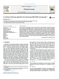
magnetometer axes. Both b and d frames are shown in Fig. 1. The rotation sequence has been parameterized by Euler angles ψ , θ and φ , respectively about body axes Zb, Yb, and Xb, thus rotating a vector representation from the reference frame basis to the body frame one. Note that here the inertial coordinate frame neglects Earth’s rotation rate. The reference frame has been useful for comparing the built-in magnetometer measurements with respect to the external magnetometer data. Additionally, a horizontal coordinate frame, or {Xh, Yh, Zh}, has resulted from rotating the body-fixed, table coordinate frame with Euler angles −φ and −θ about Xb, and Yb axes, respectively. The resulting horizontal frame is rotated by angle ψ about the local upward vertical with respect to the desired reference frame. This is also shown in Fig. 1.

Figure 1. Table frame (left), desired reference frame (middle) and horizontal frame (right). 2.2. Sensors The air-suspended table relies on three sensors for attitude estimation: two accelerometers and one magnetometer. The accelerometers are used to estimate the local vertical, and thus align the table with the horizontal coordinate frame. Data from the built-in magnetometer, called M1, has been compared with the output of the external magnetometer, called M2, to determine the error with respect to the reference azimuth direction about the local vertical. The two accelerometers measure the Xb ( Aspb ,1 ), and Yb ( Aspb, 2 ) components of gravity’s reaction specific force in the body-fixed, table coordinate frame, as in Eq. 1:

 Aspb,1   0   − 9,81. sin(θ )    b  Asp b =  Aspb ,2  = D d . 0  =  9,81. cos(θ ) sin(φ )   Aspb,3  9,81 9,81. cos(θ ) cos(φ )  

(1)

where D bd is the direction cosine matrix (DCM) that transforms a vector representation from the reference frame to the table coordinate frame. Accelerometer bias and measurement noise have not been considered in Eq. 1, but they have been added to validate the closed-loop control and the estimators. Both magnetometers have been assumed to be located in such way that the local magnetic field vector is practically the same at both locations. Otherwise, comparing their respective measurements would not be feasible for tracking the reference azimuth direction and the accuracy when estimating Euler angle ψ would be degraded. The magnetometer on board the air-suspended table output a vector measurement, M2b , which called for representation in the horizontal coordinate frame. That has been done with the estimated Euler angles φˆ and θˆ to approximate the DCM Dbh , as in Eq. 2.

M2 h ≈ D bd .M2b

(2)

One can compare M1h and M2b to approximate the desired Euler angle ψ , which is the angle about the local vertical that the horizontal frame must be rotated to be in alignment with the reference frame, thus yielding Eq. 3:

sin(ψ ) = M1d,2.M2 h,1 − M1d,1.M2 h,2

(3)

where Mxd , y is the y-th component of the unit-norm measurement vector produced by the x-th magnetometer. Therefore, the sensor suite described here allows for the measurement of the three Euler angles that rotate the reference coordinate frame to table frame. 2.3. Actuators A set of three actuators is used to control the air-suspended table about its three axes: two pneumatic actuators for the Xb and Yb axes, and one reaction wheel for Zb. The pneumatic actuators are controlled by a pulse width modulation


(PWM) signal that determine the on-off duty cycle. Additive white noise has been included in the actuator model to account for the small turbulence at the nozzles when torquing the table. Three parameters are called for in such a model: the torque magnitude that is applied on the table by the nozzles when the actuator is on, the frequency of the PWM carrier, and the actuator noise variance. The reaction wheel was modelled as in Sidi (1997). This model has included wheel motor dynamics, current and voltage limits, viscous friction, and the maximum angular rate limit. Zero-crossing dead-band has been discarded from this model because it can be easily avoided by assuming that the reaction wheel can be initialized with non-zero angular rate, hence becoming a biased momentum wheel, and such an initial condition does not affect the results. The corresponding block diagram can be seen at Fig. 2, where I m is the wheel inertia, I m,3 is the table inertia around the Zb axis, K m , K v , Rm and B are electromechanical wheel parameters, Tw is the commanded torque, and u3 is the real torque. The wheel angular rate with respect to the air-suspended table can be measured by an embedded tachometer in the device. This measurement is ωtac and it is composed of ωbwb ,3 plus white-noise.

Figure 2. Reaction wheel block diagram. 2.4. Dynamic system model The dynamic system model was adapted from Sidi (1997). The table inertia matrix without the reaction wheel I m, b , and the reaction wheel inertia matrix I w,b , both represented in the body-fixed table coordinate frame b, are shown in Eqs. 4.

I m,b

 I m,b,1  =  I m,b ,2,1  I m,b,3,1 

I m,b ,1,3   I m,b, 2,3  I m,b,3 

I m,b,1,2 I m,b, 2 I m,b,3, 2

I w,b

 I w,b ,1  =  I w,b ,2,1  I w,b,3,1 

I w,b,1,2 I w,b ,2 I w,b,3, 2

I w,b,1,3   I w,b, 2,3  I w,b,3 

(4)

The table angular rate vector with respect to the inertial frame represented in the b coordinate frame ω bi b , and the reaction wheel angular rate vector with respect to the table represented in the same coordinate frame ω bwb are shown in Eqs. 5:

[

bi bi bi ωbi b = ωb ,1 ωb , 2 ωb ,3

]

T

[

ωbwb = 0 0 ωbwb ,3

]

T

(5)

Based on a Newtonian approach, the dynamic model is represented in the table coordinate frame b as in Eq. 6:

ω& bbi,1   I m, b,1 + I w,b,1  bi   ω& b, 2  =  I m, b,2,1 + I w,b, 2,1 ω& bi   I +I  b,3   m, b,3,1 w,b,3,1

I m,b,1,2 + I w, b,1, 2 I m , b , 2 + I w, b , 2 I m, b,3,2 + I w, b,3,2

  −1 I m, b,1,3   0   I m,b, 2,3  .(−I w,b . 0  − ω bi b × H b + Tc , b + Td , b )  u3  I m, b,3   I w, b,3 

(6)

where Td ,b is the disturbance torque, Tc,b is the control torque output by the pneumatic actuators and shown in Eq. 7,

H b is the total angular momentum of the table and the reaction wheel as in Eq. 8, and u3 is the actual torque acting on the reaction wheel as shown at Fig. 2. Unbalance torque due to gravity has been disconsidered since the testbed is assumed to have undergone a balancing procedure to align the mass center with the table air bearing.

[

Tc,b = Tc,b,1 Tc ,b, 2

]

0T

(7)


wb H b = (I m, b + I w,b ).ω bi b + I w, b .ω b

(8)

The table angular rate vector ω bi b relates to the attitude kinematics given by the Euler angles ψ , θ , and φ time derivatives according to Eqs. 9:

& = ω bi + sin(φ ) tan(θ )ω bi + cos(φ ) tan(θ )ω bi Φ b ,1 b,2 b ,3

θ& = cos(φ )ωbbi, 2 − sin(φ )ωbbi,3 ψ& =

(9)

sin(φ ) bi cos(φ ) bi ωb, 2 + ωb,3 cos(θ ) cos(θ )

Hence, the complete model has been constructed using Eqs. 6, 8, 9, and the reaction wheel model seen in Fig. 2. 3. MODEL STATE AND MEASUREMENT VECTORS Analyzing the model equations in the previous section, a vector state with seven real components has been defined: the three Euler angles that rotate from the reference frame to the body-fixed table frame, the three components of the angular rate vector of the table with respect to the inertial frame, and the reaction wheel speed with respect to the table. Static friction torque in the vicinity of the reaction wheel zero speed yields a steady-state pointing error about the Zb axis. Therefore, the integral of such pointing error, shown in Eq. 10, has been selected to augment the state vector as the eighth state component as seen in Eq. 11.

ε=

t

∫ (ψ 0

ref

− ψ )dt → ε& = ψ ref − ψ

[

x= φ θ ψ

(10)

ωbbi,1 ωbbi, 2 ωbbi,3 ωbwb,3 ε

]

T

(11)

The reference state is given by Eq. 12. Thus, the controller should align the table with the local horizontal plane, and likewise the on-board magnetometer measurement components with those of the external magnetometer.

x ref = [0 0 0 0 0 0 0 0]T

(12)

Recalling Eq. 3, the measurement vector concatenates accelerometers, magnetometers and tachometer data as in Eq. 13.

 Aspb,1 y = −  9,81

Aspb, 2 9,81

 M1d,2.M2 h,1 − M1d,1.M2 h,2 ωtac  

T

(13)

4. CONTROL STRATEGY The main focus is to investigate and compare the performance of two nonlinear estimators. Consequently, a straightforward control technique based on state feedback has been used. Firstly, the system has been linearized around x ref . As a result, the horizontal plane dynamics given by state components φ , θ , ωbbi,1 and ωbbi, 2 has become decoupled from the vertical dynamics embedded in the remaining state components. Such decoupling allowed for the design of two separate state feedback control laws for the horizontal and vertical dynamics, respectively. Then, the closed-loop poles in Eqs. 14 have been located to avoid actuator saturation while still yielding an acceptable settling time.

p horizontal = [− 1 − 1 − 1,5 − 1,5]

p vertical = [− 0,2 + j 0,2 − 0,2 − j 0,2 − 0,15]

(14)

Additionally, each horizontal axis control is turned off when the corresponding Euler angle error norm is less than 0,25°, and the control is switched back on when this error is higher than 0,5°. This avoids high-frequency switching in actuators when the system is near the reference. 5. ESTIMATORS Given the nonlinear model, an Extended Kalman Filter (EKF) and an Unscented Kalman Filter (UKF) have been compared to gauge the performance in terms of estimation accuracy and computational load. This section describes


details about the implementation of both estimators. The filters assumed a set of model simplifications. The disturbance torques have been considered nonexistent, the inertia matrices of table and reaction wheel considered diagonal, i.e., without inertia products, and the reaction wheel dynamics have been neglected, i.e. Tw = u3 . 5.1. Extended Kalman Filter (EKF) The EKF performs the linearization of the dynamical equation about the updated state estimate and the linearization of the measurement equation about the propagated state estimate (Ristic et. al, 2007). The model dynamics and measurement equation, omitting model and measurement noise, can be written as in Eqs. 15:

x& = f (x, u )

y = h( x)

(15)

where u is a vector containing commanded torques for both pneumatic actuators and the reaction wheel, and f (.) is a function concatenating Eqs. 4 to 10 considering the aforementioned simplifications. The EKF has been implemented using the continuous-discrete approach. As a result, state estimate propagation method has been accomplished by integrating the model dynamics between measurement samples using xˆ k −1|k −1 as the initial condition, as in Eq. 16:

xˆ k | k −1 = xˆ k −1| k −1 +

∫

tk

f (x, u)dt

(16)

t k −1

The error estimation covariance is propagated as in Eq. 17 using Pk −1|k −1 as the initial condition:

Pk | k −1 = Pk −1| k −1 +

∫

tk

t k −1

(J f (x, u)P (t ) + P(t )J f (x, u)T + Q(t ))dt

(17)

where J f (x, u) is the Jacobian matrix of the function f (.) at the point (x, u) , and Q is the model noise covariance matrix. Both integrations have used the Runge-Kutta 4th-order algorithm. The update has been based on linearizing the measurement equation as in Eq. 18:

y k ≈ J h (xˆ k |k −1 ).(x − xˆ k|k −1 ) + h(xˆ k|k −1 ) = J h (xˆ k|k −1 ).x − J h (xˆ k|k −1 ).xˆ k|k −1 + h(xˆ k|k −1 )

(18)

Therefore, the Kalman update step can be summarized as in Eqs. 19:

xˆ k |k = xˆ k |k −1 + K k ( y k − h( xˆ k |k −1 )) K k = Pk |k −1 J h (xˆ k |k −1 ).(J h (xˆ k |k −1 )Pk |k −1 J h (xˆ k |k −1 ) T + R k ) −1

(19)

Pk |k = (I − K k J h (xˆ k |k −1 )).Pk |k −1 5.2. Unscented Kalman Filter (UKF) The UKF uses the unscented transform to achieve a better estimation than the EKF if the process is highly nonlinear. The unscented transform calculates a set of σ-points that are propagated using the nonlinear model and measurement equations to estimate the mean and covariance of the stochastic state vector (Ristic et. al, 2004). Unlike the EKF, it does not need computation of Jacobians. Nevertheless, the computing of σ-points requires a great amount of computational effort, which makes this method slower than the first in almost every practical situation. The UKF has been also used along the continuous-discrete approach (Särkkä, 2007). So, the state propagation uses the unscented integration with xˆ k −1|k −1 as the initial condition, as in Eqs. 20: tk

xˆ k|k −1 = xˆ k −1|k −1 +

[ γ (t ) = [f (σ (t ), u)

∫ γ(t ).W dt m

tk −1

]

[

σ (t ) = σ1 (t ) σ 2 (t ) ... σ 2.na +1 (t ) = [x(t ) x(t ) ... x(t )] + na + κ . 0 na x1 M

[

1

Wm = W1m W2m

f (σ 2 (t ), u) ... f (σ 2.na +1 (t ), u) ... W2m.na +1

]

T

W1m =

]

κ na + κ

Wi m =

P (t ) M − P(t )

1 → 1 < i ≤ 2na + 1 2.(na + κ )

]

(20)


where na is the number of states, κ is a tuning factor in which 3 is optimal for Gaussian noise, and P(t ) is the square root matrix of P (t ) computed as the lower triangular matrix in the Cholesky factorization. The covariance propagation is as in Eqs. 21, where Pk −1|k −1 is the initial condition (Särkkä, 2007): tk

∫

Pk|k −1 = Pk −1|k −1 +

(Ω(t ) + Ω(t )T + Q(t ))dt

Ω(t ) =

2.na +1

∑W

i

m

.(σ i (t ) − x(t )).(γ i (t ) − γ (t ).Wm )T

(21)

i =1

t k −1

The above integration uses the Runge-Kutta 4th-order algorithm, whereas the UKF update is given in Eqs. 22 (Ristic et. al, 2004):

[

]

σ k |k −1 = σ k | k −1,1 σ k |k −1,2 ... σ k | k −1, 2.n a +1 =

[

]

[

= xˆ k | k −1 xˆ k | k −1 ... xˆ k | k −1 + na + κ . 0 n a x1 M

[

γ k = h (σ k | k −1,1 ) h (σ k | k −1,2 ) ... h(σ k | k −1, 2.n a +1 ) yˆ k =

2.n a +1

∑W

m

i

i =1 2.n a +1

Pzz , k =

Pxz , k =

.γ k ,i

2.n a +1

∑W

m

i

]

Pk | k −1 M − Pk | k −1

]

.(σ k −1,i − xˆ k | k −1 ).(γ k , i − yˆ k |k −1 )T

(22)

i =1

∑W

m

i

.( γ k ,i − yˆ k | k −1 ).(γ k ,i − yˆ k | k −1 )T

S k = R k + Pzz , k

K k = Pxz , k S k−1

i =1

xˆ k | k = xˆ k | k −1 + K k (y k − yˆ k )

Pk | k = Pk | k −1 − K k S k K Tk

6. SIMULATIONS 6.1. Parameters The simulations have been carried out using table parameters from Carrara and Milani (2007), and XSens MTiG IMU specification sheet. Table 1 shows the used values. Ground-truth inertia matrices of the table and reaction wheel have included inertia products to account for a residual assembly mass unbalance. Equation 23 shows the measurement noise covariance matrix used in both filters: 2 2 2 2 R = diag (σ accel . / 9,81 σ accel . / 9,81 4.σ mag / 500 σ tac )

(23)

where diag (.) means a diagonal matrix. The model noise covariance needed to be separately tuned for each filter to avoid divergence during the simulation. The selected values for the EKF and UKF is in Eq. 24:

Q ext = 0,5.I 8 x8

Q usc = 0,45.I 8 x8

(24)

6.2. Filter performance Two metrics have been defined to gauge filter performance. The first computes the rotation angle about the Euler axis that is related to the attitude estimation error at each iteration as in Eq. 25. It has been used to ascertain the attitude estimation accuracy of each filter. The second computes the norm of the angular rate vector estimation error at each iteration as in Eq. 26.

1 ˆ b,T .Db ) − 1 ) Θ error , k = a cos( .trace(D d d , k |k 2 2

(25)

ˆ k|k − ωk ) t (ω ˆ k|k − ωk ) ωerror ,k = (ω

(26)

b ˆb where D d , k | k and D d are the estimated and true direction cosine matrices, respectively, at instant k that rotate from the

reference coordinate frame to the table coordinate frame, and ωˆ k |k and ω k are the estimated and true table angular rate vector, respectively, at instant k. These two metrics have been computed at each iteration over a large number N of Monte Carlo simulations. At the end, the mean and standard deviation have been computed.


Table 1. Parameters used at simulation. Symbol

h I m,b

I w, b

Bl

ε accel. 2 σ accel .

Description

Value General Sample time 0,01 s Table inertia matrix, without the reaction wheel,  0,4954 / 2 0,4954.0,1 − 0,4954.0,1 represented in table coordinate frame  0,4954.0,1 0,4954 / 2 0,4954.0,05  kg.m 2  − 0,4954.0,1 0,4954.0,05 0,4954  Reaction wheel inertia matrix represented in  1,5.10 −3 / 2 1,5.10 −3.0,1 − 1,5.10 −3.0,1 table coordinate frame   −3 −3 −3 2  1,5.10 .0,1 1,5.10 / 2 1,5.10 .0,05 kg.m − 1,5.10− 3.0,1 1,5.10 − 3.0,05 1,5.10 − 3    Local magnetic field represented in the [0,8729 − 0,4364 0,2182]T .500 mGauss reference coordinate frame Sensors Accelerometer bias 1 mg Accelerometer measurement noise variance (0,002. 30 ) 2 (m / s 2 ) 2

2 σ tac

Tachometer measurement noise variance

0,005 V 2

2 σ mag

Magnetometer measurement noise variance

(0,5. 10 ) 2 (mGauss ) 2

σ 2p

Actuators Maximum torque output by the pneumatic 0,1 N.m actuators Pneumatic actuator torque noise variance 0,1 / 1000 ( N .m) 2

fp

Pneumatic actuator PWM carrier frequency

2 Hz

ωbwb , max

Reaction wheel maximum angular rate

4200 rpm

Twmax

Reaction wheel maximum torque

0,05 N.m

Km

Reaction wheel motor constant

0,023 V / A

ic, sat

Reaction wheel current saturation

Twmax / K m A

Rm

Reaction wheel motor resistance

10 Ω

Vc, sat

Reaction wheel voltage saturation

Rm .ic, sat V

K c, pi

Proportional gain in reaction wheel PI controller

10

I c , pi

Integral gain in reaction wheel PI controller

2

Bw

Reaction wheel viscous friction coefficient

4,9.10 −6

K v, w

Reaction wheel K v back-emf coefficient

1.10 −3 V .s / rad

Tpmax

6.3. Results For each scenario described below, 100 Monte Carlo simulations have been carried out in a time interval from 0s to 100s. The initial state vector has been kept fixed and given in Eq. 27 with SI units. For each simulation, the filter initial estimate has been set equal to the initial state vector plus a random vector in which each component was a random Gaussian variable with zero mean and variance 0.1.

x 0 = [25.π / 180 − 30.π / 180 20.π / 180 3.π / 180 − 3.π / 180 − 2.π / 180 0 0]T [SI units]

(27)

An unexpected, deterministic disturbance torque has been applied at t=45s to investigate filter behavior and convergence. The applied torque vector is given in Eq. 28.

Td ,b = [− 0,7 0,7 0,3]T N .m

(28)

The first scenario used the EKF as the estimator. The results are plotted in Fig. 3. The second scenario used the UKF and the results are shown in Fig. 4. Figure 5 plots the mean errors of the first and second scenarios together. The


mean filter algorithm simulation time in the first approach was 4.8136s with a standard deviation of 1.096s. The mean filter algorithm simulation time in the second approach was 9.6889s with a standard deviation of 0.8601s. Figure 6 shows that the UKF has yields more accurate attitude estimates after the unexpected disturbance. At the first peak, the UKF error corresponded to only 64.6% error of the EKF’s. However, the corresponding computational load in the UKF was 101.3% higher. In steady state, the estimation error produced by the two filters was quite similar. Then, a third scenario was simulated in which the EKF is used during usual operation and switches to the UKF at t=46s using the updated state estimation and covariance from the EKF. This procedure attempts to reproduce a condition in which the control system embeds a fault detection, diagnosis, and reconfiguration scheme that takes 1s to identify the disturbance and then switch accordingly from the EKF to the UKF. The mean filter algorithm simulation time was 7.4007s with a standard deviation of 0,5088s. Finally, a comparison between the first and third scenarios is plotted in Fig. 6.

Figure 3. Scenario 01 results – Extended Kalman Filter.

Figure 4. Scenario 02 results – Unscented Kalman Filter.


7. CONCLUSIONS Two nonlinear estimation techniques have been investigated for use in a simulated air-suspended table subject to a straightforward, linearized state feedback law for attitude control. The table uses two pneumatic actuators for alignment with the local horizontal plane, and one reaction wheel for azimuth alignment. The sensors consist of two accelerometers to estimate the local gravity vector direction, and two magnetometers - one on board the table, and the other fixed to the inertial coordinate frame to provide azimuth alignment about the local vertical. The nonlinear system dynamics have been linearized around the desired state, thus decoupling horizontal and vertical dynamics. The state feedback control has successfully allocated the closed-loop poles in the desired locations for each of the decoupled dynamics. Three scenarios have been simulated with an unexpected deterministic torque disturbance. The first one used an Extended Kalman Filter, the second used an Unscented Kalman Filter, whereas the third used the EKF that switched to the UKF after the disturbance has been detected. The UKF showed more accurate attitude estimation after the disturbance in comparison with the EKF, but the estimation quality of both in steady-state was quite similar. Thus, since the UKF had a computational load 101.3% higher than the EKF, a switch from the EKF to the UKF was proposed in case a disturbance occurs after a steady-state interval. This hybrid EKF-UKF scenario produced an error very similar to the second scenario but with a computational load only 53.7% higher than the EKF-only approach. One should notice though that this investigation has not considered any fault detection and diagnosis scheme to automatically produce the aforementioned switching. Such scheme is definitely a factor to contribute to the computational load of the hybrid approach. The UKF exhibited a behavior less robust to parameter tuning than the EKF. When the filter tuning parameters were not fine tuned, numerical errors arise and remove the positive definiteness of the estimation error covariance matrix. This loss of positive definiteness causes the square root matrix computation in Eq. 22 unfeasible. The EKF approach also exhibited divergence when its tuning parameters filter were not appropriately tuned, though the acceptable intervals for variation of such parameters were found to be quite large. Finally, the UKF provided an estimation gain when compared to the EKF, and such can be an interesting feature in some applications. The heavier computational load can be reduced with a hybrid approach as described in the third scenario, though it calls for the additional computations in a fault detection and diagnosis algorithm. Future investigation should focus on finding ways to avoid the problem encountered regarding the covariance matrix square root calculation in the UKF, thus adding to filter robustness to numerical errors in a real application. Advancing further towards more recent nonlinear filtering, e.g. the particle filters, future investigation into filter performance under disturbance occurrences seems an attractive avenue, since the computational power of embedded computing resources is increasing each day and may render the usage of more sophisticated filters in real aerospace applications.

Figure 5. Comparison between the first and second scenarios.


Figure 6. Comparison between the first and third scenarios. 8. ACKNOWLEDGEMENTS The authors acknowledge the support provided by project FINEP/CTA/INPE SIA (Sistemas Inerciais para Aplicação Aeroespacial). We also thank INPE researchers Dr. Valdemir Carrara and Dr. Helio Koiti Kuga, for the information, data and help provided. 9. REFERENCES Carrara, V., Milani, P. G., 2007, “Controle de uma Mesa de Mancal a Ar de um Eixo Equipada com Giroscópio e Roda de Reação”, Proceeding of V Simpósio Brasileiro de Engenharia Inercial, Vol. 31, pp. 97-102. Ristic, B., Arulampalam, S., Gordon, N., 2004, “Beyond the Kalman Filter: particle filters for tracking applications”, Ed. Artech House, Boston, United States of America, pp. 3-32. Sidi, M. J., 1997, “Spacecraft Dynamics and Control: a practical engineering approach”, Ed. Cambridge University Press, New York, United States of America, pp. 160-164. Särkkä, S., 2007, “On Unscented Kalman Filtering for State Estimation of Continuous-Time Nonlinear Systems”, IEEE Transactions on Automatic Control, Vol. 52, No. 9, pp. 1631-1641. 10. RESPONSIBILITY NOTICE The authors are the only responsible for the printed material included in this paper.