Nonlinear Functions for Blind Separation and Equalization - CiteSeerX

Series in Signal and Information Processing Volume 7

Diss. ETH No 14313

Nonlinear Functions for Blind Separation and Equalization

A dissertation submitted to the Swiss Federal Institute of Technology, Zürich for the degree of Doctor of Technical Sciences

presented by

Heinz Mathis dipl. El.-Ing. ETH born on March 31, 1968 citizen of Küblis GR

Hartung Gorre Konstanz

accepted on the recommendation of Prof. Dr. Hans-Andrea Loeliger, examiner Prof. Dr. Scott C. Douglas, co-examiner Hartung-Gorre Verlag, Konstanz, November 2001

Für Franziska

Die Liebe ist langmütig, die Liebe ist gütig. Sie ereifert sich nicht, sie prahlt nicht, sie bläht sich nicht auf. Sie handelt nicht ungehörig, sucht nicht ihren Vorteil, lässt sich nicht zum Zorne reizen, trägt das Böse nicht nach. Sie freut sich nicht über das Unrecht, sondern freut sich an der Wahrheit. Sie erträgt alles, glaubt alles, hofft alles, hält allem stand. Die Liebe hört niemals auf. 1. Korinther 13,4–8

Acknowledgments I would like to thank Prof. G. S. Moschytz for providing such an excellent research environment with an academic freedom second to none and for inviting me to join his group. I would also like to thank his successor, Prof. H.-A. Loeliger, for acting as the referee of this thesis and for letting me continue with my ideas. Furthermore, I thank Prof. S. C. Douglas for acting as a co-referee and for hosting me as a guest researcher at the Southern Methodist University in Dallas during Summer 2001. The signal and information processing laboratory (ISI) is a fantastic group to be a member of. I learned a lot from many different people and would like to thank them all for sharing their experience with me. The biggest thanks I owe to Marcel Joho, who got me acquainted with the subject of blind separation and with whom I shared many interests, largely due to the similar pace at which our families were growing. But my thanks also goes to Thomas von Hoff, whose publications on the stability analysis greatly influenced the direction of this thesis, to Pascal Vontobel for solving many a mathematical puzzle, to Hanspeter Schmid, Felix Lustenberger, and Stefan Moser for working out solutions to my Latex problems, and to Max Dünki for providing a stable Unix environment. I would like to thank all the people who ran with me at lunch-times, in particular Markus Helfenstein, who really pushed me up that hill. I am also thankful to people with whom I could discuss non-work-related problems, in particular to Sigi Wyrsch and Dani Lippuner. The people who proof-read this thesis have earned special acknowledgment for their endurance: Elsabe van den Heever, and again Marcel Joho and Thomas von Hoff. My deepest thanks, however, goes to my family. I thank my parents for their constant support and encouragement throughout all the stages of my education. iii

iv

Acknowledgments

I also thankfully remember the times I spent studying up in the Alps with my lovable Grandmother, Nani, who sadly passed away during the time I wrote up this thesis. I am deeply grateful to my wife, Franziska, for all her love, patience, support, and encouragement, and to my two boys, Lars and Roman, for simply being there.

Abstract Nonlinear functions are an important part of blind adaptive algorithms solving filtering problems such as blind separation and blind equalization. Roughly speaking, they take over the role of a proper training reference signal, which is not available, hence the term “blind”. The common idea shared by stochastic gradient-search algorithms either separating or deconvolving signals (or both) is to cross-correlate the signals before and after a nonlinear function, which reveals any existing higher-order correlation among the signals or among different time lags of the same signal. Such higher-order correlations indicate mutual dependence, which is then formed into an error signal to drive the output signals toward a state of higher independence. The underlying higher-order statistics are implicitly produced by the nonlinear functions. These nonlinear functions are essentially defined by the probability density function of the original source signals to extract and the cost function (such as mutual independence, maximum-likelihood, etc.). In cases where the original distributions are unknown, change over time, or are of different nature, the nonlinearity has to adapt itself according to some estimate of the distribution, or be robust enough to cover a wide mismatch of the assumed model. Stability analyses reveal the stable regions of nonlinearities by determining the set of distributions for which a given nonlinearity results in local separation convergence. Unfortunately, no fixed nonlinearity can cover the entire universe of distributions. Although the exact form of the nonlinearity might not matter for an algorithm to converge, it may have an impact on the convergence time of the separation/deconvolution process. By investigating these stability and performance parameters, robust, optimal, and universal (parametric) nonlinearities can be found. If complexity is an issue, simple nonlinearities are preferable v

vi

Abstract

to nonlinearities employing hyperbolic or polynomial functions. The threshold nonlinearity is such a simple nonlinearity. It works directly for sub-Gaussian signals such as typically used in digital data communications. Moreover, by adjusting the threshold, it may be used to separate any non-Gaussian signal. Bias removal techniques, which remove any coefficient bias due to additive noise, are applicable to the threshold nonlinearity. The threshold nonlinearity is also well suited to blind equalization and blind carrier phase synchronization, a technique that is related to blind signal separation, and can hence be described within a common framework. On the other hand, many simple algorithms for blind deconvolution, such as Sato’s algorithm and the constant-modulus algorithm (CMA) can be extended to work for a wider class of distributions by adding a simple coefficient norm factor in the update equation.

Keywords: Blind signal separation, blind equalization, blind carrier phase synchronization, nonlinear functions, threshold nonlinearity.

Kurzfassung Nichtlineare Funktionen spielen eine bedeutende Rolle in der Lösung von Filterungsproblemen wie blinde Quellenseparierung bzw. blinde Egalisation mit adaptiven Algorithmen. Grob ausgedrückt übernehmen sie die Rolle eines Trainingssignales, welches bei blinden Methoden fehlt. Das fundamentale Prinzip von stochastischen Gradientensuchalgorithmen für die Separation oder die Rückfaltung von Signalen (oder beides gleichzeitig) beruht auf der Kreuzkorrelation der Signale vor und nach der Nichtlinearität, welche vorhandene Korrelationen höherer Ordnung unter den Signalen oder zu verschiedenen Zeitpunkten eines Signals aufzeigt. Solche Korrelationen höherer Ordnung weisen auf Abhängigkeiten hin und werden daher in ein Fehlersignal umgeformt, welches das System in einen Zustand höherer statistischer Unabhängigkeit führt. Die zu Grunde liegenden Statistiken höherer Ordnung werden implizit generiert durch die nichtlinearen Funktionen, die im wesentlichen gegeben sind durch die Wahrscheinlichkeitsdichtefunktionen der originalen Quellensignale und durch die gewünschte Kostenfunktion (wie z.B. statistische Unabhängigkeit, Maximum-Likelihood, usw.). In Fällen mit unbekannter oder wechselnder Quellenverteilung, oder unterschiedlicher Verteilung der verschiedenen Quellensignale, muss die Nichtlinearität an eine Schätzung der Quellenverteilung adaptierbar sein, oder sie muss robust genug sein, um eine grobe Abweichung des angenommenen Modells tolerieren zu können. Stabilitätsanalysen erlauben die Angabe einer Stabilitätsregion einer Nichtlinearität, indem sie die Menge der Quellenverteilungen ermitteln, für die eine gewisse Nichtlinearität lokale Konvergenz liefert. Keine fixe Nichtlinearität deckt die Gesamtheit aller Quellenverteilungen ab. Obwohl die genaue Form der Nichtlinearität nicht entscheidend für stabile Konvergenz sein muss, hat sie doch entscheidenden Einfluss auf die Konvii

viii

Kurzfassung

vergenzzeit des Separations- oder Rückfaltungsprozesses. Durch die Analyse von Stabilitätsbedingungen und Konvergenzverhalten können robuste, optimale und universelle (parametrisierbare) Nichtlinearitäten gefunden werden. Wenn Komplexität ein Designkriterium ist, sind einfache Nichtlinearitäten solchen die hyperbolische oder Polynomfunktionen verwenden, vorzuziehen. Die Schwellwert-Nichtlinearität ist eine solche einfache Nichtlinearität. Sie funktioniert direkt für sub-gauss’sche Signale, wie sie typischerweise in Kommunikationssystemen vorkommen. Mittels Adaption des Schwellwertes kann sie zur Separation eines beliebigen nicht-gauss’schen Signals verwendet werden. Techniken, die wegen additivem Rauschen eingehandelte Verschiebungen der Lösung (Bias) korrigieren, lassen sich kombinieren mit der SchwellwertNichtlinearität. Die Schwellwert-Nichtlinearität eignet sich ebenfalls für blinde Egalisation und für blinde Trägerphasensynchronisation, eine Technik die eng verwandt ist mit blinder Quellenseparierung und daher mit ähnlicher Notation beschrieben werden kann. Auf der anderen Seite können viele einfache Algorithmen für die blinde Egalisation, wie z.B. Sato’s Algorithmus oder der Constant-Modulus Algorithmus, mittels Hinzufügen eines Koeffizientennormterms in der Aufdatierungsgleichung auf eine breitere Klasse von Verteilungen angewendet werden.

Stichworte: Blinde Quellenseparation, blinde Kanalegalisation, blinde Trägerphasensynchronisation, nichtlineare Funktionen, Schwellwert-Nichtlinearität.

Contents Abstract

v

Kurzfassung

vii

1 Introduction 1.1 Motivation . . . . . . . . . . 1.2 Historical development . . . 1.2.1 Blind deconvolution 1.2.2 Blind separation . . 1.3 Contributions of the thesis . 1.4 Outline of the thesis . . . . .

. . . . . .

. . . . . .

. . . . . .

. . . . . .

. . . . . .

. . . . . .

. . . . . .

. . . . . .

. . . . . .

. . . . . .

. . . . . .

. . . . . .

1 1 2 3 4 5 6

2 Statistical prerequisites 2.1 Statistical moments and cumulants . . . . 2.1.1 Definitions . . . . . . . . . . . . 2.1.2 Kurtosis of a signal . . . . . . . . 2.2 Source distributions . . . . . . . . . . . . 2.2.1 Continuous distributions . . . . . 2.2.2 Discrete distributions . . . . . . . 2.2.3 Complex continuous distributions 2.3 Moment ordering . . . . . . . . . . . . . 2.4 Properties of the kurtosis . . . . . . . . . 2.4.1 Motivation . . . . . . . . . . . . 2.4.2 Minimum kurtosis . . . . . . . . 2.4.3 Sum kurtosis . . . . . . . . . . . 2.4.4 Influence of timing offsets . . . . 2.4.5 SNR estimation . . . . . . . . . . 2.5 Summary . . . . . . . . . . . . . . . . .

. . . . . . . . . . . . . . .

. . . . . . . . . . . . . . .

. . . . . . . . . . . . . . .

. . . . . . . . . . . . . . .

. . . . . . . . . . . . . . .

. . . . . . . . . . . . . . .

. . . . . . . . . . . . . . .

. . . . . . . . . . . . . . .

. . . . . . . . . . . . . . .

. . . . . . . . . . . . . . .

. . . . . . . . . . . . . . .

9 9 9 11 12 12 16 20 21 27 28 28 31 32 37 38

. . . . . .

3 Blind signal separation

. . . . . .

. . . . . .

. . . . . .

. . . . . .

. . . . . .

39 ix

x

Contents

3.1

Problem formulation . . . . . . . . . . . . . . . . . . . . 3.1.1 Model and assumptions . . . . . . . . . . . . . . 3.1.2 Performance measures . . . . . . . . . . . . . . . 3.1.3 Narrowband model . . . . . . . . . . . . . . . . . 3.1.4 Relationship to beamforming . . . . . . . . . . . . 3.2 Maximum-likelihood solution . . . . . . . . . . . . . . . 3.3 Accelerated update equation . . . . . . . . . . . . . . . . 3.3.1 Natural/relative gradient . . . . . . . . . . . . . . 3.3.2 Alternative derivation of the gradient modification 3.4 Convergence behavior . . . . . . . . . . . . . . . . . . . . 3.5 Equilibrium points . . . . . . . . . . . . . . . . . . . . . 3.6 Other cost functions . . . . . . . . . . . . . . . . . . . . . 3.6.1 Entropy maximization / information maximization 3.6.2 Negentropy . . . . . . . . . . . . . . . . . . . . . 3.6.3 Mutual information . . . . . . . . . . . . . . . . . 3.6.4 The EASI algorithm . . . . . . . . . . . . . . . . 3.6.5 CMA and kurtosis . . . . . . . . . . . . . . . . . 3.6.6 Semiblind signal separation . . . . . . . . . . . . 3.7 Stability conditions . . . . . . . . . . . . . . . . . . . . . 3.7.1 Stability analysis for complex-valued signals . . . 3.7.2 Stability regions of some nonlinearities . . . . . . 3.8 Overdetermined signal separation . . . . . . . . . . . . . 3.9 Other modifications . . . . . . . . . . . . . . . . . . . . . 3.10 Summary . . . . . . . . . . . . . . . . . . . . . . . . . . 4 Nonlinear functions 4.1 Introduction . . . . . . . . . . . . . . . . . . . . . . . 4.2 Gaussian sources . . . . . . . . . . . . . . . . . . . . 4.3 Scaling the nonlinearity . . . . . . . . . . . . . . . . . 4.4 Convergence speed of the BSS algorithm . . . . . . . 4.5 Monomial functions . . . . . . . . . . . . . . . . . . . 4.5.1 QAM signals . . . . . . . . . . . . . . . . . . 4.5.2 Monomials for complex baseband signals . . . 4.6 Optimal nonlinearities . . . . . . . . . . . . . . . . . 4.6.1 The form of the nonlinearity . . . . . . . . . . 4.6.2 Optimization of the nonlinearity . . . . . . . . 4.7 A proof of the nonexistence of a universal nonlinearity 4.7.1 The polynomial nonlinearity . . . . . . . . . . 4.7.2 Problem statement . . . . . . . . . . . . . . . 4.7.3 Stability analysis . . . . . . . . . . . . . . . . 4.7.4 Difficult distributions . . . . . . . . . . . . . . 4.8 Stabilizing blind separation algorithms . . . . . . . . .

. . . . . . . . . . . . . . . .

. . . . . . . . . . . . . . . .

. . . . . . . . . . . . . . . . . . . . . . . .

. . . . . . . . . . . . . . . . . . . . . . . .

40 40 43 43 44 44 47 47 48 49 51 52 53 55 56 57 57 58 62 62 66 69 71 71

. . . . . . . . . . . . . . . .

. . . . . . . . . . . . . . . .

73 74 74 75 77 77 79 80 82 82 83 85 85 85 86 90 93

Contents

xi

4.9

96

Summary . . . . . . . . . . . . . . . . . . . . . . . . . . . .

5 The Threshold Nonlinearity 97 5.1 Formal derivation of the score function for the uniform distribution . . . . . . . . . . . . . . . . . . . . . . . . . . . . . . 98 5.2 The threshold nonlinearity as a score function . . . . . . . . . 100 5.3 Stability analysis . . . . . . . . . . . . . . . . . . . . . . . . 101 5.3.1 Continuous distributions . . . . . . . . . . . . . . . . 101 5.3.2 Discrete distributions . . . . . . . . . . . . . . . . . . 108 5.3.3 Complex-valued baseband signals . . . . . . . . . . . 111 5.4 Computer simulations . . . . . . . . . . . . . . . . . . . . . . 112 5.4.1 Uniformly distributed signals . . . . . . . . . . . . . 112 5.4.2 M-QAM signals . . . . . . . . . . . . . . . . . . . . 112 5.5 The threshold nonlinearity as a universal parametric nonlinearity 115 5.6 Stabilization of arbitrary distributions . . . . . . . . . . . . . 119 5.6.1 Known methods . . . . . . . . . . . . . . . . . . . . 119 5.6.2 The adaptive threshold nonlinearity . . . . . . . . . . 122 5.6.3 Output normalization . . . . . . . . . . . . . . . . . . 122 5.6.4 Advantages of the new method . . . . . . . . . . . . . 126 5.6.5 Computer simulations . . . . . . . . . . . . . . . . . 126 5.7 Separating in an AWGN channel . . . . . . . . . . . . . . . . 129 5.7.1 Unbiased blind separation . . . . . . . . . . . . . . . 129 5.7.2 MMSE vs. zero-forcing solution . . . . . . . . . . . . 132 5.7.3 Computer simulations . . . . . . . . . . . . . . . . . 133 5.8 Summary . . . . . . . . . . . . . . . . . . . . . . . . . . . . 135 6 Blind equalization/deconvolution 6.1 Introduction . . . . . . . . . . . . . . . . . . . . . . . . 6.1.1 Motivation . . . . . . . . . . . . . . . . . . . . 6.1.2 Classification of algorithms . . . . . . . . . . . 6.2 Problem formulation . . . . . . . . . . . . . . . . . . . 6.2.1 Model and assumptions . . . . . . . . . . . . . 6.2.2 Performance measure . . . . . . . . . . . . . . . 6.3 Traditional Bussgang-type algorithms . . . . . . . . . . 6.3.1 The Sato algorithm . . . . . . . . . . . . . . . . 6.3.2 Godard’s algorithm . . . . . . . . . . . . . . . . 6.3.3 The constant-modulus algorithm (CMA) . . . . . 6.3.4 The Benveniste-Goursat-Ruget (BGR) algorithm 6.3.5 Benveniste-Goursat’s algorithm . . . . . . . . . 6.3.6 The Stop-and-Go Algorithm . . . . . . . . . . . 6.3.7 Other criteria . . . . . . . . . . . . . . . . . . . 6.3.8 Summary of algorithms . . . . . . . . . . . . .

. . . . . . . . . . . . . . .

. . . . . . . . . . . . . . .

. . . . . . . . . . . . . . .

137 137 138 139 140 140 141 142 142 143 143 144 145 145 146 146

xii

Contents

6.4 6.5

6.6 6.7

Increased convergence speed . . . . . . . . . . . . . . An extension to Bussgang-type algorithms . . . . . . . 6.5.1 Introduction . . . . . . . . . . . . . . . . . . . 6.5.2 Local stability analysis . . . . . . . . . . . . . 6.5.3 Stability for generalized Gaussian distributions 6.5.4 Algorithm modifications . . . . . . . . . . . . 6.5.5 Examples . . . . . . . . . . . . . . . . . . . . 6.5.6 Computer simulations . . . . . . . . . . . . . Natural-gradient updates . . . . . . . . . . . . . . . . 6.6.1 The threshold nonlinearity . . . . . . . . . . . Summary . . . . . . . . . . . . . . . . . . . . . . . .

7 Blind carrier phase synchronization 7.1 Introduction . . . . . . . . . . . . . . . . . . . . . . . 7.1.1 Vestigial sideband modulation . . . . . . . . . 7.2 Phase-error induced symbol error rates . . . . . . . . . 7.2.1 SER of PAM with phase error . . . . . . . . . 7.2.2 SER of QAM with phase error . . . . . . . . . 7.2.3 SER of VSB with phase error . . . . . . . . . 7.2.4 Symbol error floor . . . . . . . . . . . . . . . 7.3 Residual phase-error correction . . . . . . . . . . . . . 7.3.1 Data-aided phase-error correction . . . . . . . 7.3.2 Blind phase synchronization . . . . . . . . . . 7.3.3 Blind phase-error correction for 8-VSB system 7.4 Simulation results . . . . . . . . . . . . . . . . . . . . 7.5 Summary . . . . . . . . . . . . . . . . . . . . . . . .

. . . . . . . . . . . . . . . . . . . . . . . .

. . . . . . . . . . . . . . . . . . . . . . . .

. . . . . . . . . . . . . . . . . . . . . . . .

. . . . . . . . . . .

146 149 149 149 156 157 160 163 166 166 167

. . . . . . . . . . . . .

169 170 170 171 171 172 172 176 176 177 177 181 185 188

8 Concluding remarks 189 8.1 Conclusions . . . . . . . . . . . . . . . . . . . . . . . . . . . 189 8.2 Outlook . . . . . . . . . . . . . . . . . . . . . . . . . . . . . 190 A Functions and formulae A.1 The Gamma function . . . . . . . . . . . . . . . . . . . . . . A.2 Stirling’s formula . . . . . . . . . . . . . . . . . . . . . . . . A.3 Matrix-Inversion Lemma . . . . . . . . . . . . . . . . . . . . A.4 Differentiation with respect to a matrix of complex elements . A.5 Derivation of the relationship between the fourth-order cumulant and higher-order moments . . . . . . . . . . . . . . . . .

193 193 194 194 195 196

B Constellations and SERs of some digital modulation formats

197

C Formal proofs

199

Contents

C.1 Proofs of the lemmas on the kurtosis of a sum of two independent signals . . . . . . . . . . . . . . . . . . . . . . . . . . . C.2 A lemma on the expectation of a product of two functions . . . C.3 Proof of Eq. (2.34) . . . . . . . . . . . . . . . . . . . . . . . C.4 Proof of Eqs. (2.44) and (2.45) . . . . . . . . . . . . . . . . .

xiii

199 201 204 205

Abbreviations

207

List of Symbols

211

Bibliography

215

Index

227

About the Author

235

Chapter 1

Introduction 1.1

Motivation

Situations where information signals occur corrupted either by time-shifted replicas of their own signal or by other signals of similar nature can be found in the real world in a vast variety. Reverberation of acoustic signals in closed rooms, multipath propagation in wireless communications, blurred images, low-pass-filtered biomedical signals, to name just a few, are all examples illustrating the prevalence of unwanted convolution in different areas. Similarly, the problem of simultaneous excitations of multiple sources has applications in acoustics, communications, biomedical engineering, image processing, and even data mining (extraction of information or knowledge from data bases). Whereas the human brain can handle the so-called “cocktail-party effect” quite successfully, engineers have battled to devise algorithms resolving such situations. In the wireless-communication world, recent government auctions of frequency bands have clearly indicated the need to make optimum use of the bandwidth available. Besides traditional approaches such as TDMA, FDMA, and CDMA, multiple use of common channels is possible using space division multiple access (SDMA), where the fact is exploited that no two transmitters or receivers have the same physical location. The basic configuration of a wireless communication system with several transmitters and receivers sharing the same channels can be visualized by Fig. 1.1. 1

2

Chapter 1. Introduction transmitters

channels

receivers

BSS algorithm

s1

..

sn

un mixing process

A

The notion of blind deconvolution appeared for the first time in [121] and describes the problem of deconvolving two signals when both are unknown. Stockham’s method required the idea of homomorphic signal processing, a summary of which can be found in [107]. In short, homomorphic systems are nonlinear systems that obey a generalized principle of superposition. Homomorphic signal processing is particularly useful when two signals that are convolved are constitutionally different.

separation process

W

Figure 1.1: Multichannel wireless communication system. Modern communication systems increasingly require training-less adaptation, either to save capacity, due to multipoint considerations in broadcast environments, or to accommodate unpredictable channel changes [135]. So-called self-recovering or blind algorithms are useful here, since they operate without the knowledge of some training sequence. Although blind algorithms reach back as far as 30 years, it has only become an area of intense research activities over the last ten years. The new wave of research of blind algorithms has been motivated by two main factors. First, new fast-converging methods [7] have been discovered, based on informationtheoretical concepts [12, 86]. Second, the semiconductor industry has developed new hardware systems that allow the real-time implementation of such algorithms.

1.2

3

1.2.1 Blind deconvolution

u1

..

1.2. Historical development

Historical development

Historically, the problem of blind deconvolution appeared much earlier than blind separation. This is on the one hand due to suitable methods to blindly separate signals, which became available later than their counterpart for blind deconvolution, but on the other hand also due to a rising number of applications of MIMO (multiple in—multiple out) systems in recent years. Despite the fact that the two problems are related in nature and many applications require the simultaneous solution of both problems—so-called multichannel blind deconvolution (MCBD)—we separately list their respective historical development.

In the seventies and eighties, research into blind deconvolution was mainly driven by two areas. On the one hand the oil industry heavily subsidized projects investigating the analysis of geophysical layerings, which blind deconvolution was widely applied to, but with relatively few disclosed publications. On the other hand many pioneers in blind deconvolution had their roots in communications, which consequently was an area to which many original papers were devoted. If decision-directed algorithms are regarded as blind algorithms—they do not assume knowledge of the input symbols, but estimate them—Lucky [91] certainly deserves to be mentioned as one of these pioneers. Very often, however, Sato [117] is considered the father of blind deconvolution algorithms in the form that represents the counterpart of the nonblind LMS stochasticgradient update rule. At that time it was already clear that by using a nonlinear function, higher-order terms are implicitly generated, whose statistical independence are necessary in the most general case, rather than second-order independence or decorrelation only. A very similar algorithm to Sato’s algorithm was devised independently by Godard [60] and by Treichler and Agee [126], and became subsequently known as either Godard’s algorithm in its more general case or the so-called constantmodulus algorithm (CMA), which is still used today. The expression blind equalization, which has become a standard term in communications, was first used by Benveniste and Goursat [17]. They and other researchers [113] combined different error functions to get a smooth changeover from a blind to a decision-directed mode. Alongside with the development of algorithms, there was a quest for sufficient and necessary conditions for blind equalization, so subsequently many results were of existential rather than constructive nature, i.e., they did not explicitly lead to the solutions, but provided the necessary framework in terms of

4

Chapter 1. Introduction

conditions and assumptions, and increased the insight of solutions known at the time and to follow later. Among the first researchers to state sufficient conditions for perfect equalization were Benveniste et al. [18], who showed that the original signal is retrieved if the probability density function (pdf) of the deconvolved sequence matches that of the original signal. Later, Shalvi and Weinstein [120] relaxed this condition by showing that perfect equalization is achieved by maximizing the output kurtosis.

1.2.2 Blind separation

Blind signal separation (BSS), also referred to as blind source separation, is a much younger research topic than blind deconvolution. The conference publications by Hérault and Jutten [67] followed by the their journal publication [77] are usually regarded as the seminal papers in blind signal separation. The nonlinearities used in their approach were, however, found more heuristically than with mathematical rigor. Furthermore, they used a recurrent neural network as opposed to later approaches, which mostly concentrated on feed-forward networks. Jutten and Hérault [77] also came up with the term Independent Components Analysis (INCA), which later became more standard as Independent Component Analysis (ICA) [36]. Subsequently, ICA has been used as an equivalent of BSS, but strictly speaking, ICA is more a method to solve the BSS problem. With ICA, a paradigm evolved that let many researchers think about the true cost function to minimize. In this spirit, cost functions motivated by information theory arose. The key papers of this concept were written by Bell and Sejnowski [11, 12]. A further milestone in the development of fast blind separation algorithms was the introduction of a modified gradient, which led to considerably shorter convergence times. Amari [2] and Cardoso [22] independently derived solutions that resulted in the same update equation for the adaptive algorithm, and named their method natural gradient and relative gradient, respectively.

1.3. Contributions of the thesis

1.3

5

Contributions of the thesis

The main subjects of this thesis are blind adaptive algorithms, in particular for signal separation, with an emphasis on suitable nonlinearities, which reveal dependencies among different signal parts (either temporal or spatial), and help drive such dependencies to zero. Special focus is set on the following topics: • A concise treatment of higher-order moments, in particular fourth-order statistics (kurtosis) with respect to their influence on the behavior of blind adaptive algorithms is provided. The influence of timing offsets of digitally modulated signals to their kurtoses is of special interest. Moment relations of a large class of distributions can be expressed with respect to the Gamma function. Using the convex property of the Gamma function allows the derivation of many useful relationships of higher-order moments of those distributions. • The thesis contains a systematic overview of current blind separation algorithms and a comparison of their respective convergence times. Whereas the literature usually states the stability conditions for realvalued random variables, the more general conditions for complex values are derived here. • Unlike most approaches, which exclude noise, the true ML gradientsearch update equation for an AWGN channel is derived and put into relation to the more famous noiseless case. Furthermore, the application of bias removal techniques to the threshold nonlinearity algorithms is investigated. • Working nonlinearities are categorized according to their suitability and complexity. The score function is shown to maximize robustness against model mismatch. It was previously assumed that universal nonlinearities for all possible distributions do exist. It is shown in this thesis that any approach to find such a fixed nonlinearity is inherently flawed. • A very attractive nonlinear function in the form of a threshold nonlinearity is introduced that has favorable features such as low computational complexity. By introducing a parameter into this three-level quantizer, a universal parametric nonlinearity is created, which separates any nonGaussian distributions, a fact that is proven in this thesis. Stability criteria for continuous and discrete distributions are derived. Making the threshold parameter adaptive allows the devising of an algorithm to separate

6

Chapter 1. Introduction

unknown distributions. There are also distributions that the “classical” nonlinearities fail to separate, but where the threshold nonlinearity succeeds. • Many of the properties of blind equalization can be deduced from those of blind signal separation. Furthermore, sufficient conditions for local stability of Bussgang-type blind equalizers are derived, and extensions of such equalizers, which are normally designed to work for sub-Gaussian signals, to more general distributions are presented. • The intimate relationship of blind signal separation and blind phase synchronization is yet another topic. The application of blind phase synchronization to HDTV signals confirms its usefulness.

1.4

Outline of the thesis

In Chapter 2 we deal with the statistical prerequisites for blind adaptive signal processing. Besides definitions and characteristics of moments and cumulants, and the introduction of some parametric distributions, we derive some important features of the kurtosis. The formulation of the blind signal separation problem is a substantial subject of Chapter 3. We derive an adaptive maximum-likelihood solution, which will accompany us throughout the thesis. Other criteria are shortly treated and the stability conditions are reviewed. Chapter 4 deals with nonlinear functions as used in blind adaptive algorithms. Their relevance to different distributions is investigated, and their resulting convergence properties are compared. In this chapter we also show a new justification for the score function, and provide a proof of the nonexistence of universal fixed nonlinearities for the separation of all non-Gaussian distributions. Finally, we offer a list of possible solutions to stabilize blind separation algorithms. The main result of this thesis is the construction of a simple, piece-wise constant nonlinearity with properties similar to those of more complicated functions. The so-called threshold nonlinearity is the main topic of Chapter 5. We formally derive this nonlinear function from the uniform distribution and indicate its suitability to other distributions by studying its stability regions. In this context, discrete distributions are of particular interest, as they have many potential applications in data communications. The most fundamental result of

1.4. Outline of the thesis

7

this chapter is the proof of the stability of the threshold nonlinearity for any non-Gaussian signal for a properly chosen threshold value. By adapting this value, we devise an algorithm that separates a mixture of distributions with different kurtosis signs. Other extensions of the algorithm mitigate bias effect due to AWGN on the transfer medium. Blind equalization, a problem that is in fact older than blind separation, is the theme of Chapter 6. We give an overview of Bussgang-type algorithms, investigate their stability regions, and present a means of extending such algorithms to the class of super-Gaussian signals. The use of the threshold nonlinearity in natural-gradient algorithms for blind deconvolution rounds off this chapter. Chapter 7 consists of a treatment of blind phase synchronization algorithms, which can be regarded as a special case of blind separation algorithms. Their usefulness is demonstrated at the example of HDTV signals. Finally, Chapter 8 contains the conclusions and some outlook on possible further research activities in the area of this thesis. A collection of formulae used in this thesis and some formal proofs can be found in the Appendix.

Chapter 2

Statistical prerequisites Statistical quantities play an important role in blind signal processing in the construction of algorithms, their control, and their performance evaluation. It seems therefore appropriate to collect the necessary tool set into an introductory chapter. We first note the definitions of moments and cumulants and in particular the most important cumulant in blind signal processing—the normalized fourth-order cumulant or in short the kurtosis—in Section 2.1. In Section 2.2 probability density functions of some sources used in blind problems are shortly introduced and their respective kurtoses are given. An important feature of moments that is later used in Chapter 5 is moment ordering, which is introduced in Section 2.3. Salient properties of the kurtosis, such as the minimum kurtosis, the sum kurtosis, the influence of non-ideal sampling time on the kurtosis, and SNR estimation by the sample kurtosis are the subjects of Section 2.4.

2.1

Statistical moments and cumulants

2.1.1 Definitions In the following we shall give some important definitions with respect to nonlinear moments and cumulants of random variables. The nth moment of a random 9

10

Chapter 2. Statistical prerequisites

2.1. Statistical moments and cumulants

11

2.1.2 Kurtosis of a signal

variable x is given by Mx(n) , E x n =

Z

∞ −∞

x n px (x) d x.

Often, the central moments are required, which are given by Z ∞ (n) n ˜ Mx , E (x − m x ) = (x − m x )n px (x) d x. −∞

(2.1)

(2.2)

(1)

m x , Mx is the linear expectation of x, and for m x = 0, the two definitions of the moments coincide. The moments can also be computed through the characteristic function, which is given by n o Z ∞ jt x φ(t) , E e = e jt x px (x) d x. (2.3)

The kurtosis, which is simply the normalized fourth-order cumulant, belongs to the more important quantities used to describe a statistical variable. Particularly in blind signal processing, kurtosis plays a significant role, but other areas such as SNR estimation can also benefit from some of the properties of the kurtosis. For the rest of this thesis except for Section 2.4.4 we assume i.i.d. signals . We therefore use the terms signal and variable interchangeably apart from in the aforementioned section. The kurtosis of a real random variable x is essentially given by its normalized fourth-order central moment. Two different definitions are commonly used, namely E |x − m x |4 κ˜ 4 , (2.11) σx4

−∞

and

The nth moment of x is then given by Mx(n)

d n φ(t) = (− j) . dt n t=0 n

(2.4)

Intimately related to the characteristic function is the cumulant generating function, given by n o K (t) , ln φ(t) = ln E e jt x . (2.5) The nth cumulant can be computed as C x(n)

d n K (t) = (− j) dt n n

.

(2.6)

t=0

(n)

(n)

Relationships between Mx and C x may be formed [103] and are particularly easy for zero-mean, symmetrically distributed random variables. In this case we have C x(1) = 0, C x(2) C x(3)

=

(2.7)

Mx(2) ,

= 0,

(2.8)

C x(4) = Mx(4) − 3 Mx(2)

(2.9)

2 .

For a derivation of Eq. (2.10), see also Appendix A.5.

(2.10)

κ4 ,

E |x − m x |4 − 3, σx4

(2.12)

with m x and σx2 denoting the mean and variance of the random variable x, respectively. We stick to the latter definition, since it exhibits a couple of interesting properties. With Eq. (2.12), the kurtosis of symmetrical distributions corresponds to the fourth-order cumulant, normalized by the squared variance, as can be seen by inspection of Eq. (2.10). Gaussian variables have a zero kurtosis (mesokurtic), so that the sign of the kurtosis determines subor super-Gaussianity. Haykin [66] writes that although perhaps in an abusive way, a random variable is said to be sub-Gaussian or super-Gaussian if the kurtosis is negative or positive, respectively. Super-Gaussian signals have a positive kurtosis, and are also called leptokurtic, while sub-Gaussian signals have a negative kurtosis, and are referred to as platykurtic. Although super- and sub-Gaussianity were originally reserved [18] for pdfs of the form p(x) = K exp (−g(x)), for even g(x), and were determined by the asymptotic behavior of g 0 (x)/x, the connection between Gaussianity and kurtosis has found wide acceptance in the converse direction, too. Note that as we shall later see, Gaussianity is a sufficient but not necessary condition for distributions to be mesokurtic. In the following, we assume zero-mean variables, i.e., m x = 0. For complex signals, different definitions of the kurtosis are in use [138]. One possible definition is the same as for real signals (cf. Eq. (2.12)). Another, often used definition for the kurtosis of a zero-mean complex random variable

12


is given by [120] κ40

2 2 E |x|4 − 2 E |x|2 − E x 2 , . σx4

E |x|4 − 2, σx4

13

A large family of signals can be modeled using the generalized Gaussian distribution [13], whose pdf is given by

(2.13)

For distributions exhibiting some circular symmetry we have E x 2 = 0, so that Eq. (2.13) turns into κ40 ,

2.2. Source distributions

(2.14)

which is just 1 higher than the value obtained by Eq. (2.12), i.e., κ40 = κ4 + 1. Strictly speaking, the true condition for E x 2 = 0 is that the real and imaginary parts of the random variable are statistically uncorrelated and have the same second-order moment. Many researchers have tried to find intuitive explanations of what kurtosis exactly indicates, similarly to how one explains variance as deviation from its mean. Two notions have arisen, peakedness combined with tailedness, and bimodality. However, to either concept counter-examples were found by Darlington [38] and Hildebrand [68], respectively. Still, for most distributions in use, both intuitive grasps show their validity. A high kurtosis usually implies strong peakedness combined with tailedness in the pdf, or sometimes also called lack of shoulder. A low kurtosis on the other hand indicates high bimodality. The relationship between the form of the pdf and the kurtosis sign has been further investigated in [58].

px (x) =

α − e 1 2β0 α

|x| α β

,

(2.15)

where the parameters α and β determine the shape and the variance of the distribution, respectively. 0(.) denotes the Gamma function, which is defined in Appendix A.1. Distributions of the form given by Eq. (2.15) with 0 < α < 2 are referred to as super-Gaussian, those with α > 2 as sub-Gaussian distributions. For a plot of the Gamma function and other details, see Appendix A.1. Special values of the parameter α lead to some very common distributions, e.g., α = 1 makes Eq. (2.15) the Laplacian distribution, α = 2 the Gaussian, and α = ∞ the uniform. Table 2.1 shows the calculation of the moments as a function of the parameters. E {|x| p }

distribution

α

β

px (x)

Laplacian

1

√ 2 2 σx

px (x) =

√1 2σx

px (x) =

√ 1 2π σx

Gaussian

uniform

2 ∞

√ √ s

general

α

2σx

3σx

px (x) =

0 α1 σx 0 α3

Eq. (2.15)

√ |x| 2 σx

e− e

2 − x2 2σ x

|x| ≤ β 0, otherwise

1 2β ,

0( p + 1) 0 p+1 2 0 12

√

√

2 2 σx

p

p 2σx

√ p 3σx p+1

0 p+1 α 0 α1

βp

Table 2.1: Moments of the generalized Gaussian distribution.

2.2

Source distributions

2.2.1 Continuous distributions Beside the many given fixed distributions for specific physical sources, parametric source distributions, which cover a whole range of different models are frequently used, since they allow viability checking and comparison of algorithms under different circumstances.

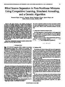
For the generalized Gaussian distribution, the parameter α determines the kurtosis in the following way [62] 0 α5 0 α1 κ4 = 2 − 3. (2.16) 0 α3 The kurtosis of the generalized Gaussian distribution is not upper bounded for α → 0, but lower bounded by −1.2 for α → ∞ (uniform distribution). Fig. 2.1

14



(upper left) and Fig. 2.2 visualize the distribution given by Eq. (2.15) and the kurtosis given by Eq. (2.16), respectively.

generalized Gaussian 0.8

Only unimodal signals can be expressed by the generalized Gaussian distribution given by Eq. (2.15). However, digital data signals are mostly bimodal or multimodal. The two-tailed Gamma distribution [68], whose pdf is

0.6

βα px (x) = |x|α−1 e−β|x| , 20(α)

−∞ < x < ∞,

(2.17)

can model a wider range of distributions than the generalized Gaussian family. Some calculations involving this family, however, tend to be more difficult, due to the simultaneous appearance of a power of x and the exponential function in the density function. For α = 1, Eq. (2.17) too expresses the Laplacian distribution. Pitfalls are lurking when handling the numerical representation of the pdf of the two-tailed Gamma distribution for extreme values of the parameter α. Using Stirling’s formula (see Appendix A.2), we can find an approximation of Eq. (2.17) for large values of α, r 1 α α(1−|x|+ln |x|)−ln |x| px (x) = , −∞ < x < ∞, α 1, (2.18) e 2 2π which avoids some numerical problems associated with large terms. Table 2.2 shows the calculation of the moments as a function of the parameters. The distribution and the kurtosis as a function of the parameter α are again shown in Fig. 2.1 (upper right) and Fig. 2.2, respectively. distribution

α

β

Laplacian

1

√ 2/σx

binary

∞

∞

α

√ (α + 1)α · σx

general

E {|x| p }

px (x) √1 2σx

√ |x| 2 σx

e−

δ(x−σx ) 2

x) + δ(x+σ 2

Eq. (2.17)

0( p + 1)

√

2 2 σx

p

p

σx

The two-tailed Gamma distribution exhibits a kurtosis as given by (α + 3)(α + 2) − 3. (α + 1)α

0.2

two−tailed Gamma 0.8 0.6

α=1 α=2.3 α=10

0.4 0.2

0 −5

0

0 −5

5

symmetric Beta 4

α=0.1 α=0.5 α=1 α=10

3 2

0

5

unbiased, symmetric Beta 1

α=0.01 α=1 α=10

0.5

1 0 −0.5 0 0.5 1 1.5

0 −2

0

2

Figure 2.1: pdfs of some parametric distributions. If only sub-Gaussian signals are of interest, a possible parametric distribution can be obtained from the symmetric Beta distribution [68, 116], which is given by 0(2α) α−1 ˜ α−1 , x˜ (1 − x) 0 2 (α)

0 < x˜ < 1.

(2.20)

Shifting and scaling of Eq. (2.20) leads to an unbiased, symmetric Beta distribution 0(2α) 1 x 1 α−1 1 x α−1 px (x) = 2 · · , −β/2 < x < β/2, + − β 2 2 β 0 (α) β (2.21)

Table 2.2: Moments of the two-tailed Gamma distribution.

κ4 =

α=1 α=2 α=4 α=105

0.4

˜ = px˜ (x)

0(α+ p) 0(α)β p

15

(2.19)

We see that this distribution can model signals with a kurtosis all the way down to −2, hence unimodal and bimodal signals.

where the parameter β as with the other two pdfs depends on the variance of the signal, and is given by √ β = 2 2α + 1σx . (2.22)

16



17

1 The following signals are deterministic ones, so that the term “distributions” refers to the amplitude density rather than the probability density.

V.29 (cf. [105])

M = 16

1 ring with 2 points (BPSK) 1 ring with 4 points (QPSK) 2 rings with 4 points 2 rings with 8 points 4 rings with 8 points 4 rings with 16 points M = 2: M = 4: M = 8: M = 16: M = 32: M = 64: variable-rate star QAM (cf. [133])

M ≥4 m=1

M π 1 X δ x − e j(2m−1) M , M

M-PSK

(odd power of 2)

n=1 m=1

Table 2.3: Kurtoses of digitally modulated signals.

κ4 = −1.58

κ40 = −0.58

N/A κ4 = −2.00 κ4 = −2.00 κ4 = −1.36 κ4 = −1.36 κ4 = −1.65 κ4 = −1.65

κ40 = −2.00 κ40 = −1.00 κ40 = −0.36 κ40 = −0.36 κ40 = −0.65 κ40 = −0.65

−1.00 κ40 = −1.00

−2.00

=

κ4 = −2.00

−0.65 ·

−1.65

259M 2 −64 (31M−32)2

− 12 5 κ40

2

−9920M+2048 κ4 = − 7913M 5·(31M−32)2

48 31M − 32 amplitude for unit energy:

r M-QAM

Baseband representations of sampled, digitally modulated signals have discrete distributions rather than continuous forms as treated in the previous section.

Signal

2.2.2 Discrete distributions

M-PAM

pdf

m=1 √ √ M/2 X M/2 X

hence reaches from zero (Gaussian) to −2 (binary). Its dependency on α is also depicted in Fig. 2.2.

δ

(2.26)

r

The kurtosis of unbiased, symmetric Beta distributed signals is given by

Finally, the kurtosis of some other continuous distributions1 of interest are −1.5 for a sine wave, −1.2 for a triangular or sawtooth signal (same as uniform distribution), and again −2 for a rectangular pulse signal (same as BPSK signal).

−0.60

−1.60 q x−(±(2m−1)± j(2n−1))

! 3 2 M −1

n=0

κ4 = −6/(2α + 3),

2 4M − 1 κ4 = − · 5 M −1 3 M +1 κ40 = − · 5 M −1 3 2(M−1)

the moments of the unbiased, symmetric Beta distribution, which is again depicted in Fig. 2.1, are then given by E x p = E (β(x˜ − m x˜ )) p p X p−n p = βp (−1)n E x˜ n m x˜ n n=0 p p n− p 0(α + n) 0(2α) p X = (−1)n 2 β . (2.25) n 0(α) 0(2α + n)

1 M

(2.24)

M/2 1 X δ x ± (2m − 1) M

0(α + p) 0(2α) E x˜ p = , 0(α) 0(2α + p)

M-QAM

Since the moments of the symmetric Beta distribution px˜ (.) are given by [116]

6 M2 + 1 κ4 = − · 2 5 M −1

α 1. (2.23)

lim κ4 , κ40

α 1 x 1 α−1 1 x α−1 , · · + − π β β 2 2 β − β/2 < x < β/2,

M→∞

px (x) = 2

kurtosis

r 2α−1

−1.20

For large α, the fraction of two Gamma functions is numerically unstable, so using Stirling’s formula again we can rewrite Eq. (2.21) into

18


3

generalized Gaussian two-tailed Gamma symmetric Beta M-PAM M-QAM

2.5 2 1.5 1

κ4

0.5

super−Gaussian

0 sub−Gaussian

−0.5 −1 −1.5 −2 −1 10

0

10

10

1

2

10

α, M Figure 2.2: Kurtoses of generalized Gaussian, two-tailed Gamma, and symmetric Beta distributed signals (all vs. α), M-PAM signals (vs. M), and M-QAM signals (vs. M).

Their kurtoses can be calculated in closed form from their probability distributions2 using Eq. (2.12). The results are given in Table 2.3, and plots of the kurtoses for PAM (pulse amplitude modulation, also referred to as amplitude shift keying or short ASK) and QAM (quadrature amplitude modulation) are depicted in Fig. 2.2. Note that both definitions of the kurtosis of a complex signal (Eqs. (2.12) and (2.13)) are given in Table 2.3. An interesting point arises for M-PAM as M approaches infinity. As we steadily increase the number of possible values of the source variable and therefore the modality, the kurtosis approaches −1.2, the kurtosis for a uniform distribution, which is referred to as being nonmodal by Hildebrand [68]. For square QAM constellations, M needs to be a square of an integer. However, other constellations are possible, and are used in current technology, e.g., the voice modem standards V.32 and V.33 use 32-QAM and 128-QAM, respec-


19

tively. Because an odd power of two can always be written as M = 22m+1 = 22m−2 · 23 = (2m−1 )2 · (32 − 1) = (2m−1 · 3)2 − (2m−1 )2 ,

a difference of two squares, each of which is divisible by four for integer values of m ≥ 2, a constellation can always be built where a large square is pruned by four small corner squares, e.g., for 32-QAM we skip the four corner points of a 36-point square (m = 2). The exact kurtosis of such constellations, also referred to as cross constellations, lacks the easy form of square constellations but can still be expressed in closed form as given in row 3 of Table 2.3. A similar table containing the kurtoses of digitally modulated distributions can be found in [123]. An interesting case of a signal whose kurtosis does not monotonously increase with growing M is the variable-rate star QAM as suggested by Webb and Hanzo [133]. Their method of increasing the data rate is based on doubling alternately the number of amplitude rings and the number of points per ring in the constellation. For two rings, the two amplitudes are in the ratio of three-to-one. With four rings, the 1st (inner most) and 4th ring stay the same as with two rings, the other two amplitudes are chosen such that the Euclidean distances between the 2nd and 3rd, and between the 3rd and 4th ring are equal, and at the same time preserve the average energynfrom smaller constellations. o √ √ 1 −3+2 41 √ The resulting amplitudes (power normalized) are √ , , 6+√ 41 , √3 . 5

5 5

5 5

5

The kurtosis is an indicator of the convergence speed of blind adaptive algorithms. Due to higher absolute values of the kurtosis, it is easier to separate star-QAM signals with M = 2, 4, 32, 64 than with M = 8, 16. This is of course only true for blind methods that make use of the kurtosis as an independence measure. If decision-directed methods are employed, whose performance are directly related to the symbol error rate, fewer constellation points facilitate faster convergence times. In order to have a parametric discrete distribution covering a wide range of the kurtosis, we introduce a ternary distribution with Pr(x = 1) = Pr(x = −1) = p and Pr(x = 0) = 1 − 2 p. The kurtosis of this variable depends on p in the following way κ4 =

2 For discrete distributions we should refer to the distribution as a probability mass function. However, to get a consistent terminology, we still use the term probability density with additional δ(.) operators to reflect the discrete support of such densities.

(2.27)

1 − 3. 2p

(2.28)

This family of distributions covers the whole kurtosis range from ∞ to −2 as p goes from 0 to 12 . For p = 16 we get zero kurtosis. Although this choice of

20


2.3. Moment ordering

2.3

p makes the signal closest to a Gaussian distribution, other than fourth-order cumulants need not necessarily be zero.

As M grows, the QAM distributions resemble more and more those of continuous ones, or at least modeling such discrete distributions by complex, continuous distributions becomes more accurate. Some important complex, continuous distributions are listed in Table 2.4.

pdf

complex Gaussian

x R2 + x I2 1 − σ2 x p(x) = e πσx2

complex uniform

cyclic uniform

pdf plot

p(x) ( =

1 6σx2

|x R |, |x I | ≤

0

otherwise

p(x) ( =

q

κ4

For m = 2, Eq. (2.29) gives

κ40 or

−1

0

3 2 σx

1 2πσx2

x R2 + x I2 ≤ 2σx2

0

otherwise

−1.6

− 53

−0.6

− 23

Table 2.4: Some complex, continuous distributions and their respective kurtoses.

Moment ordering

Consider n˘ a unit-variance Gaussian variable n˘ ∼ N (0, 1) and x the generalized Gaussian variable given by Eq. (2.15) parameterized by α, which is larger (smaller) than 2 for sub- (super-) Gaussian signals. We will also consider a nor˘ The value of the parameter β can be found from malized version of x, called x. the general expression for the mth-order moment of a generalized Gaussian signal [84] m+1 0 α βm . E |x|m = (2.29) 0 α1

2.2.3 Complex continuous distributions

name

21

n o 0 α3 E |x|2 = β 2 0 α1

(2.30)

v u u0 1 α u β = t σx , 0 α3

(2.31)

a result already used in Table 2.1. By using α = 2 in Eqs. (2.29) and (2.30) we have the following relationship between the even moments of the unit-variance Gaussian variable o n m ˘ ˘ m−2 . E |n| (2.32) = (m − 1)E |n| Similarly, for the even moments of generalized Gaussian variables with unit variance we can find m+1 1 m 0 0 ˘ } α α E {|x| = · . (2.33) ˘ m−2 E |x| 0 m−1 0 3 α

α

The moments of any unit-variance random variable build a monotonic increasing function in m o n m ˘ ˘ m−2 , m ≥ 4, E |x| (2.34) ≥ E |x|

22


with equality if and only if x˘ is a binary random variable ∈ {±1}. A proof of Eq. (2.34) can be found in Appendix C.3. A related result to Eq. (2.34) is the corollary following the next lemma, which in turn was stated by Loève [90]. It will be used subsequently in Chapter 6.

L EMMA 2.1 For the higher-order moments of a random variable x we note that o o n n E |x|a1 E |x|b−a1 ≥ E |x|a2 E |x|b−a2 , 0 < a1 < a2 ≤ b/2. (2.35) A proof of Lemma 2.1 can be found in [111, p. 343].

C OROLLARY 2.1 E |x|m+1 The ratio m−1 is a nondecreasing function in m for any distribuE |x|

tion px (.).


23

Furthermore, if x˘ is super-Gaussian distributed, we find [1] m m ˘ ˘ E |x| > E |n| , m > 2, m m ˘ ˘ E |x| < E |n| , m < 2.

(2.38)

Vice versa, for x˘ being sub-Gaussian distributed m m ˘ ˘ < E |n| , m > 2, E |x| m m ˘ ˘ E |x| > E |n| , m < 2.

(2.40)

(2.39)

(2.41)

Although stochastic ordering is also possible for fractional moments [1], we only consider even integers for m in what follows. The mth moments for m < 2 are given for completeness and will not be used further. In fact, using Eqs. (2.32) and (2.34) in Eqs. (2.38) and (2.40) we realize that o n m ˘ ˘ m−2 , x super-Gaussian distributed, E |x| (2.42) > (m − 1)E |n| o n m ˘ ˘ m−2 , x sub-Gaussian distributed. E |x| (2.43) < (m − 1)E |n| Tighter bounds can be obtained, namely n o m ˘ ˘ m−2 , x super-Gaussian distributed, E |x| > (m − 1)E |x| o n m ˘ m−2 , x sub-Gaussian distributed, ˘ < (m − 1)E |x| E |x|

(2.44) (2.45)

where in the right-hand sides of Eqs. (2.42) and (2.43) n˘ has been replaced by ˘ A proof of Eqs. (2.44) and (2.45) is provided in Appendix C.4. x.

Proof: By setting b , 2m + δ, a1 , m − 1, a2 , m + δ − 1, with δ being a small positive real number, 0 < δ ≤ 2, and rearranging Eq. (2.35) we get E |x|m+δ+1 E |x|m+1 ≥ , (2.36) E |x|m+δ−1 E |x|m−1

Most of the equalities and inequalities from Eq. (2.32) to Eq. (2.45) can be extended to distributions whose variance is unequal to one by noting that m ˘ E |x|m = σxm E |x| (2.46)

from which we conclude that E |x|m+1 /E |x|m−1 is a nondecreasing function in m.

if x˘ is the normalized version of x. In particular, the moments of a Gaussian variable n ∼ N (0, σn2 ) are related as n o E |n|m = (m − 1)E |n|m−2 σn2 . (2.47)

In fact, Eq. (2.34) can also be proved using Corollary 2.1 and noting that for m = 1 and a unit-variance random variable we have m+1 o n ˘ E |x| 2 ˘ = 1. (2.37) = E | x| ˘ m−1 E |x|

The even moments of generalized Gaussian variables with variance σx2 are related as 0 m+1 0 α1 α E {|x|m } = · σx2 . (2.48) m−1 E |x|m−2 0 0 3

m=1

α

α

24



For arbitrary distributions we have

25

10

o n E |x|m ≥ E |x|m−2 σx2 ,

α=1 α=2 α=∞

9

m ≥ 4,

(2.49)

with equality if and only if x is binary distributed. And finally, n o E |x|m > (m − 1)E |x|m−2 σx2 , x super-Gaussian distributed, n o E |x|m < (m − 1)E |x|m−2 σx2 , x sub-Gaussian distributed.

8 7

(2.50) (2.51)

m+1 ˘ E |x| ˘ m−1 } E {|x|

6 5 4 3

Both the moments and the ratio of increasing moments are strictly monotonic increasing functions for the generalized Gaussian distribution as can be seen from Figs. 2.3 and 2.4, respectively. Moreover, E {|x|m } is a convex function in m for any distribution except for the binary distribution, where it is a constant, and the E {|x|m } /E |x|m−2 is a convex function for super-Gaussian signals.

2 1 0 2

2.5

3

3.5

4

4.5

5

5.5

6

m 20

Figure 2.4: Ratio of moments for the generalized Gaussian distribution with unit variance.

α=1 α=2 α=∞

18

Another relationship between moments of the generalized Gaussian distribution will be used in Chapter 6 and bases on the following lemma.

16 14 12

L EMMA 2.2 For 0 < α < 2 and p < q the ratio of Gamma functions behaves as q+2 0 0 p+2 α α . (2.52) p < p0 α q0 αq

˘ m } 10 E {|x| 8 6 4 2 0 2

2.5

3

3.5

4

4.5

5

5.5

6

Proof: We have to show that for

m Figure 2.3: Moments for the generalized Gaussian distribution with unit variance.

f (m) ,

0

m+2 α m0 mα

(2.53)

we have f 0 (m) ,

d f (m) > 0, dm

0 < α < 2.

(2.54)

26


27

The first two factors on the RHS of Eq. (2.61) are positive for 0 < α < 2, and the difference of the two sums is

We define δ,

2.4. Properties of the kurtosis

2−α > 0, α

0 0.

The converse of Lemma 2.2, together with Lemma 2.2 itself, will be used in Chapter 3 and is presented in the following corollary.

C OROLLARY 2.2 For α > 2 and p < q the ratio of Gamma functions behaves as q+2 0 0 p+2 α α . p > p0 α q0 αq

(2.63)

Proof: The proof goes along similar lines as that of Lemma 2.2. We note that for α > 2 and from the definition given by Eq. (2.55), we have −1 < δ < 0. As a result of this, the first two factors on the RHS of Eq. (2.61) can be negative. However, they are either both negative or both positive, thus making the product positive. The sum in Eq. (2.62) is always negative for the δ indicated, making f 0 (m) negative for all m > 0.

(2.59)

n=1

where C is Euler’s constant, we can write m m 0 mα + δ m m 0 f (m) = 2 m +δ ξ +δ −ξ −δ , α α α α m 0 α

2.4 (2.60)

which leads after some calculation and using Eq. (2.59) to f 0 (m) =

m α + δ 2 m 0 mα

0

∞ m 2 + δαm X · · α2 n n=1

m α +δ m α +δ+n

−

∞ X n=1

n

m α m α +n

! .

(2.61)

Properties of the kurtosis

Beside being a key parameter in signal classification, the kurtosis of a source signal is an indicator of the separation difficulty in blind signal separation and deconvolution if moment-based criteria are employed. Whereas the maximum kurtosis is unbounded, the lower bound on the minimum kurtosis is −2. Furthermore, the kurtosis of a composite signal has bounds that depend on the kurtoses of the constituent signals [96]. The influence of sampling-time accuracy to the kurtosis of the sampled signal has a direct implication on how accurate timing has to be in order for blind algorithms still to work satisfactorily.

28


2.4.1 Motivation

In blind signal processing, the kurtosis has two major functions. Due to the Central Limit Theorem, strong mixture and convolution push a composite distribution towards the normal distribution. Recovering these signals means driving their distributions away from the normal distribution towards their original distribution, thereby separating or deconvolving the signals. This means increasing the kurtosis if the original source distribution is super-Gaussian, and decreasing the kurtosis for sub-Gaussian distributions. Hence, the kurtoses of the source signals are on the one hand a difficulty measure of the signals to separate, with a small absolute value indicating high difficulty, and the kurtoses of the separated signals, on the other hand, can serve as an objective function for the adaptation algorithm and as a convergence indicator. For the constantmodulus algorithm (CMA)—one of the most widely used blind deconvolution algorithm—the gradient of the CM cost surface is dependent on the source kurtosis [71]. Moreover, Johnson et al. [71] show the direct implication of the kurtosis to the convergence time of the CMA.


29

L EMMA 2.3 For any two symmetrical probability density functions px (.) and px˜ (.) of a random variable x with zero mean, variance σx2 , and the relations px (x) ≤ px˜ (x), for a ≤ |x| ≤ b, px (x) > px˜ (x), otherwise,

(2.64)

the fourth-order moment Mx(4) , E x 4 for the distribution px is greater than for px˜ .

For an illustration of the relationship of the pdfs, see Fig. 2.5. −b

0.4 0.35

−a

px > px˜

px < px˜

−2

−1

b

a

px > px˜

px < px˜

px > px˜

0.3

Zervas and Proakis [138] have pointed out the influence of constellation shaping on the kurtosis. However, by shaping the constellation in an effort to maximize capacity—the maximum capacity is reached for a Gaussian distribution—the signal becomes more and more difficult to separate. In this sense, the goals of fast convergence time and of high capacity are contradictory. Finally, modulation classification is yet another use of the kurtosis [123]. For further comments on the use of the kurtosis, see also [94].

0.25

p(x)

0.2 0.15 0.1 0.05 0 −3

0

1

2

3

x

2.4.2 Minimum kurtosis The fact that the lower limit of the kurtosis is −2 has been known for some time [81]. In this section we follow a slightly different route from that pursued in [81] to prove this result, which uses similar properties of crossing pdfs as a lemma proved later in the thesis. First we state a lemma on the fourth-order moment of a random variable, which was proved by Finucan [53] in 1964.

Figure 2.5: Normalized Gaussian ( px , solid line) and uniform ( px˜ , dashed line) distributions, illustrating Eq. (2.64).

Proof: Since both functions px (.) and px˜ (.) are pdfs and must therefore integrate to one, there exists a c with a ≤ c ≤ b such that Z 0

c

Z

c

px (x) d x =

px˜ (x) d x. 0

(2.65)

30


Likewise, Z

∞

Z

∞

px (x) d x =

c

px˜ (x) d x.

(2.66)


31

Proof (alternative): We use the Cauchy-Schwarz inequality n o n o E A2 E B 2 ≥ (E {AB})2 ,

(2.70)

c

with equality if and only if A = cB, c a constant. With A , (x − m x )2 and B , 1, we get

A second random variable y is now defined as 2 y , x 2 − c2 . The mean of y, E {y} =

Mx(4) − 2c2 σx2 + c4 ,

(2.68)

is greater for the px than for the px˜ distribution, because of the higher probability density px in the range |x| < a of higher y values and an equal deficiency of probability in the range a ≤ |x| ≤ c of lower y values. The same argument is true for the ranges |x| > b and c ≤ |x| ≤ b, respectively. A greater E {y} for (4) px than for px˜ is equivalent to a greater fourth-order moment Mx , since c and σx are constants. With this result, we are now ready to prove a corollary on the minimum kurtosis, which is of interest to the study of digital communications signals. C OROLLARY 2.3 (minimum kurtosis) The kurtosis of a random variable cannot be less than −2.

1 (δ(x + 1) + δ(x − 1)) . 2

Dividing both sides of Eq. (2.71) by its right-hand side, we get (4) E (x − m x )4 Mx 2 = 4 ≥ 1, σx E (x − m x )2

(2.71)

(2.72)

which is the same as (4)

κ4 =

Mx − 3 ≥ −2, σx4

(2.73)

with equality if and only if A is a constant. This, however, means that the pdf of x is concentrated at two values due to a further symmetry constraint.

2.4.3 Sum kurtosis

Proof: The value of −2 for the kurtosis of a real random variable can be achieved by a 2-PAM (pulse amplitude modulation) signal, which is equivalent to a BPSK (binary phase shift keying) signal, given by its pdf px˜ (x) =

n o n o2 E (x − m x )4 ≥ E (x − m x )2 .

(2.67)

(2.69)

The constants a, b, and c used in the proof of Lemma 2.3 are in this case equal, i.e., a = b = c = 1. The corollary follows immediately from the lemma above. Any distribution px different from px˜ (but with equal variance) has a higher probability density outside the region a ≤ |x| ≤ b, which is concentrated to a single point. Therefore, its fourth-order moment and consequently its kurtosis are higher than that of the 2-PAM distribution px˜ . An alternative proof was offered in [81] using the Cauchy-Schwarz inequality.

We will now present a lemma on the sum of two independent random variables, which is related in nature to the Central Limit Theorem, and is of interest in connection with filtered signals. L EMMA 2.4 The absolute value of the kurtosis of a sum of two independent zeromean random variables with finite variances and kurtoses all 6 = 0 is always smaller than the larger absolute value of the kurtoses of the two signals. A proof of this lemma can be found in Appendix C.1. An example shall illustrate this situation: Assume we have two independent discrete sources each having a 2-PAM distribution. The cumulants of the sum of independent signals are equal to the sum of their respective cumulants [106],

−0.8 10

Table 2.5: Kurtosis of a sum of two independent signals.

1 σ12 σ22

−κ4 (x1 + x2 ) < −κ4 (x2 )

< −κ4 (x1 )

−2 − −

−1

−1.7 1 10 −κ4 (x2 )

< −κ4 (x1 + x2 ) < −κ4 (x1 )

−2 − −

−1

0.8 10 1 κ4 (x1 + x2 ) σ22

σ22

< κ4 (x2 )

σ12

< −κ4 (x1 )

−2 + −

1

−1.6 1 10 κ4 (x2 )

σ12

< −κ4 (x1 + x2 ) < −κ4 (x1 )

−2 + −

1

−1.6 10 1 −κ4 (x1 + x2 ) < −κ4 (x2 )

σ12

σ22

σ12 σ22

< κ4 (x1 )

3 − +

−2

2.5 1 10 < κ4 (x1 ) < κ4 (x1 + x2 ) −κ4 (x2 ) σ12 σ22

3 − +

−2

1.7 10 1 2 < κ4 (x1 ) κ4 (x1 + x2 )

< κ4 (x2 )

< κ4 (x1 ) < κ4 (x1 + x2 )

3 + +

σ22

κ4 (x2 )

A proof of this lemma can also be found in Appendix C.1.

σ12

variances

L EMMA 2.5 The absolute value of the kurtosis of a sum of two independent zero-mean random variables with finite variances and equal-sign kurtoses both 6 = 0 is always higher or equal than the lower absolute value of the kurtoses of the two signals divided by two.

Up to this point we have concentrated on ideally, critically sampled signals without a timing offset. In a realistic system we may find the situation where either clock recovery has not been carried out yet or shows some residual timing offset. This will affect the effective kurtosis and makes the signals harder to be separated.

1 + +

output kurtosis

is possible. Table 2.5 shows the eight possible cases for the kurtosis of a sum of two independent signals. The stronger of the two signals in terms of power has a dominant influence on the kurtosis of the sum signal. For signals whose kurtoses have equal signs, we can develop a lower bound similar to the upper bound given by Lemma 2.4:

2.4.4 Influence of timing offsets

3

κ4 (x1 )

(2.75)

κ4 (x2 )

|κ4 (x 1 + x 2 )| < min(|κ4 (x 1 )|, |κ4 (x 2 )|) < max(|κ4 (x 1 )|, |κ4 (x 2 )|)

or

κ4 (x1 )

(2.74)

Examples

min(|κ4 (x 1 )|, |κ4 (x 2 )|) < |κ4 (x 1 + x 2 )| < max(|κ4 (x 1 )|, |κ4 (x 2 )|)

33

General relations

Note that depending on σ12 and σ22 , the respective variance for x 1 and x 2 , either case

10

σ12

σ22

Shalvi and Weinstein [120] have made use of a related result to prove that if the kurtosis is equal to the source kurtosis at the output of an equalized system, then the original signal has been recovered.

2

κ4 (x1 + x2 )

so in our case the fourth-order cumulant doubles. However, since the variance, which is nothing but the second-order cumulant, also doubles, and the kurtosis is normalized by the squared variance, the kurtosis halves, hence in accordance with both the principle of minimum kurtosis stated in Corollary 2.3 and Lemma 2.4.

2.5


σ12 σ22


κ4 (x2 )

32

34


Communication signals are often pulse shaped by a raised-cosine filter with the impulse response hk =

sin ((k + τ/T )π) cos (ρ(k + τ/T )π) , · (k + τ/T )π 1 − 4ρ 2 (k + τ/T )2

(2.76)

with ρ being the roll-off factor, 0 ≤ ρ ≤ 1. The timing offset is denoted by τ , and T is the symbol duration. The impulse response for different ρ is shown in Fig. 2.6. If a random signal can be written as a weighted sum of independent 1

impulse response

35

where κ4,in denotes the kurtosis of the input signal to the filter. For all possible values of the timing offset τ , the weighting factors h k are maximal for ρ = 0 (ideal lowpass filter). For ρ > 0, the intersymbol-interference terms are smaller as a consequence of the fact that cos (ρ(τ/T )π) cos (ρ(k + τ/T )π) τ ≥ , 0 ≤ ≤ 0.5, k = {±1, ±2, . . .}, T 1 − 4ρ 2 (τ/T )2 1 − 4ρ 2 (k + τ/T )2 (2.78) which shall not be proved here. For this filter (or any of the form given by Eq. (2.76)), the largest degradation of the kurtosis occurs for a timing offset of half a symbol (τ = 0.5T ). For τ = 0.5T , the worst-case kurtosis of the filtered signal is then given by

ρ=0 ρ=0.5 ρ=1

0.8


X sin4 ((k + 0.5)π)

0.6

k

κ4,out =

0.4

(k + 0.5)4 π 4

X sin2 ((k + 0.5)π) k

0.2

!2 · κ4,in .

(2.79)

(k + 0.5)2 π 2

Using the equalities [21] 0

sin ((k + τ/T )π) ≡ (−1)k sin (πτ/T ) , ∞ X

−0.2 −5

−4

−3

−2

−1

0

1

2

3

4

5 k=0

τ/T Figure 2.6: Impulse response of the raised-cosine filter for different roll-off factors ρ. random signals, the total nth-order cumulant is the weighted sum (with the original weights raised to the power of n) of all nth-order cumulants of the individual signals3 . For an i.i.d. process, we can therefore calculate the kurtosis of the filter output as X h 4k κ4,out =

k

X

!2 · κ4,in ,

(2.77)

h 2k

k 3 This

property, among others, is the reason why cumulants are sometimes referred to as semiinvariants.

(2.80)

1 π2 = , 2 8 (2k + 1)

(2.81)

π4 1 = 96 (2k + 1)4

(2.82)

and ∞ X k=0

in Eq. (2.79), we obtain κ4,out =

κ4,in , 3

ρ = 0, τ/T = 0.5 .

(2.83)

In fact, it can be shown that for ρ = 0, the evaluation of Eq. (2.77) yields 1 + 2 cos2 (πτ/T ) · κ4,in 3 2 + cos(2πτ/T ) · κ4,in . = 3

κ4,out =

(2.84)

36


The smallest degradation of the kurtosis occurs for ρ = 1. For this roll-off factor and the worst-case degradation (τ/T = 0.5), h k = 0 for all k but for k = 0 and k = −1. For h 0 we get by applying Bernoulli-de l’Hospital’s rule ! sin π2 cos( Tτ π) h 0 = lim 2 π · τ/T →0.5 1 − 4 Tτ 2 2 −π sin( Tτ π) = · = 0.5. (2.85) π −8 τ τ/T =0.5

T

Similarly, it can be found that h −1 = h 0 = 0.5. Thus, we get for the kurtosis transformation after Eq. (2.77) κ4,out =

κ4,in , 2

ρ = 1, τ/T = 0.5 .

(2.86)

Fig. 2.7 shows the degradation of the kurtosis caused by timing misadjustment for the raised-cosine filter with different roll-off factors ρ. Note that this degradation is only relative to the kurtosis of the distribution, and it is furthermore independent of the distribution. The ideal lowpass filter can clearly be identified as the degradation bound (Eq. (2.84)) on the kurtosis, depicted by the solid 1


37

line. For sub-Gaussian signals, Eq. (2.83) means that no matter what timing offset we have (or even if clock recovery has not yet taken place), the kurtosis is upper bounded by κ4 /3. Blind adaptive methods may therefore still be successfully applied. Valkama et al. [129] show the influence of timing offsets on the performance of a blind separation algorithm.

2.4.5 SNR estimation Signal-to-noise ratio estimation is a task frequently used in communication algorithms. In antenna diversity, if maximum-ratio combining is applied, the combination weights depend on the SNR of the individual branches. SNR also serves as a cell hand-over criterion in a cellular network. Usually, the signal strength at the receiver input serves as an indicator of the SNR, which is often justified if the latter is dominated by thermal noise of the receiver. Many other noise sources or interferers are possible, and other more meaningful measures to estimate the SNR are needed. If the noise is of Gaussian nature, and the timing is accurate, but demodulation has not yet been fully carried out, an SNR estimator can be derived using the kurtosis. To this end we observe the kurtosis of the sum of two independent signals (see Appendix C.1)

0.9

κ4 (x 1 + x 2 ) =

0.8

κ4 (x 1 )σ14 + κ4 (x 2 )σ24 (σ12 + σ22 )2

0.7 0.6

(2.87)

If we consider x 1 to be the signal of interest and x 2 additive white Gaussian noise, then by using κ4 (x 2 ) = 0 and σx2 = σ12 + σ22 , we get

κ4,out 0.5 κ4,in

s

0.4

σ12

0.3 0.2

ρ=0 0.1≤ρ≤0.9 ρ=1

0.1 0 0

.

0.1

0.2

0.3

0.4

= σx2

|κ4 (x 1 + x 2 )| , |κ4 (x 1 )|

(2.88)

from which we can arrive at the signal-to-noise ratio 0.5

τ/T Figure 2.7: Degradation of the kurtosis caused by timing misadjustment for a raised-cosine pulse-shaping filter.

SNR ,

σ12 σ22

√

|κ4 (x 1 + x 2 )| =√ . √ |κ4 (x 1 )| − |κ4 (x 1 + x 2 )|

(2.89)

If the expression for the kurtosis of the received signal r = x 1 + x 2 is replaced

38


by the sample kurtosis, we get the SNR estimate v u 1 X 2 u 1 X t ri4 − 3 ri2 N N i i d SNR = v , !2 v u u 1 X 2 u X X u 1 1 t|κ (x )| ri2 − t ri4 − 3 ri2 4 1 N N N i

i

(2.90)

i

Chapter 3

where ri denotes the ith sample of the received signal. Eq. (2.90) forms an estimator of the SNR of a signal subject to additive Gaussian noise.

2.5

Summary

Blind signal separation

Parametric distributions help model real-world signals and investigate suitability of blind algorithms, since important fourth-order statistics (kurtosis) are directly controlled by the parameter of the distribution. From all possible continuous and discrete distributions, M-PSK signals have the lowest possible kurtosis (κ4 = −2), are therefore farthest from Gaussian, and hence build the most suitable class of digitally modulated signals for blind algorithms using higher-order statistics. The kurtoses of other modulation schemes can be expressed in a parametric closed form, and are all between −2 and −0.6. If timing offsets exist, the kurtosis might be maximally degraded to 1/3 of its original value for a certain class of pulse-shaping filters. Other bounds for composite signals are intuitive regarding the Central Limit Theorem. Apart from a convergence indicator and a measure of difficulty in blind techniques, the kurtosis may be used in estimation theory. As an example, the SNR can be estimated for an additive white Gaussian noise channel using the sample kurtosis.

In a general scenario with channel noise, the blind signal separation problem, where the estimated signals are extracted from mixtures of the original signals, can only be solved in a probabilistic sense, due to the lack of knowledge of the mixing conditions. This means that we can at best answer the question as to what mixing conditions most likely produced the current observation. The answer might not be unique, but more importantly, the question often is computationally prohibitive to answer. To overcome this inaccessibility of maximumlikelihood (ML) related solutions, adaptive algorithms using stochastic gradients are employed. After the problem formulation (Section 3.1), such an adaptive stochasticgradient algorithm based on the ML rule will be introduced in Section 3.2. The natural-gradient approach has found wide acceptance as a fast variant of stochastic-gradient algorithms, and will be investigated in Section 3.3. Section 3.4 and Section 3.5 deal with the convergence behavior and equilibrium points of the separating solution, respectively. Other criteria than ML, collected in Section 3.6, lead to similar solutions, whose validity can be checked using local stability analysis, as derived in Section 3.7. In this section, stability regions of some widely used nonlinearities are also provided. Finally, overdetermined signal separation and other modifications will be treated in Section 3.8 and Section 3.9, respectively. 39

40

Chapter 3. Blind signal separation

3.1

Problem formulation

3.1. Problem formulation

41

These ambiguities are inherent properties of the problem posed rather than of the algorithms solving it, and arise if no assumptions on the variance of the source signals are made. The matrix A may be any invertible square matrix. The assumptions made on the signals and channels usually are:

3.1.1 Model and assumptions n

• The source signals are mutually independent. • At most one source signal is Gaussian distributed.

s

information sources

x

A mixing process

noise

W separation process

u

• The sources are stationary and i.i.d. (or the underlying process is unknown). information sinks

Figure 3.1: Adaptive blind signal separation system. All data paths are vectors. The problem of blindly separating an instantaneous mixture of signals can be described as follows (see also Fig. 3.1). Suppose that the information sources generate a number of signals, conveniently described by the vector s , [s1 , . . . , s Ms ]T . Through a mixing process, usually presumed linear, and therefore represented by an unknown scalar matrix A, and an additive noise vector n , [n 1 , . . . , n Ms ]T , we get the observation vector x , [x 1 , . . . , x Ms ]T at the sensors. Ms denotes the number of sources as well as the number of sensors1 . Mathematically, we describe the observed signals by x = As + n.

(3.1)

We attack the problem by attempting to find a scalar matrix W , describing the separation process, such that the signals in vector u , [u 1 , . . . , u Ms ]T are noisy replicas of the original source signals up to some ambiguities2 . These ambiguities are: • the order of the signals within vector u (permutation)

• The matrix A is a time-invariant, invertible, square matrix. • The noise signals are mutually independent and independent of the source signals. As for the noise, sometimes knowledge of σn2 is assumed. Often, as we will see, the noise is considered negligible, thus σn2 = 0 is assumed. In this case, the model of linear mixture and separation is often the one given in Fig. 3.2.

s

A

sources

x

W

sensors

mixing process

u

separated sources

separation process

Figure 3.2: Linear mixing and separation model without sensor noise.

• the magnitudes of the original source signals (scaling) • the phases of the original source signals (the signs for real-valued sources) 1 This assumption is often met in practice. We will later relax this requirement and discuss other cases. 2 The literature often refers to such replicas as wave-preserving signals, as they maintain the original waveform up to scaling, shifting, and permutation.

In the more general case of considering channel noise, the recovered signals can be written as u = W x = W ( As + n) = P s + W n.

(3.2)

If the inverse of A is desired, P , W A should approximate as closely as possible a scaled permutation matrix. Since the numbering of the sources and for

42


symmetric distributions also the sign cannot be recovered, the number of possible permutation matrices grows rapidly with the number of sources, Ms . In fact, this number is # P = M s ! · 2 Ms .

(3.3)

For illustration purposes of the large degree of freedom the number of possible permutation matrices is given in Table 3.1. Ms 2 3 4 5 6 .. . Ms 1

√ 2π Ms

#P 8 48 384 3840 46080 .. . Ms 2Ms e

Table 3.1: Number of possible permutation matrices as a function of the number of sources. The last entry is an approximation using Stirling’s formula [21].

The separation process can be modeled as a single-layer neural network (see for example [4] or [102]) with an equal number of input and output nodes, where the coefficients wi j of the separation matrix W are simply the weights from the input to the output nodes. The activation functions—the equivalent term for nonlinear function or nonlinearity in the neural network terminology— at the output nodes are used for the training mode only. For the separation process itself we restrict ourselves to the linear case. This is particularly important for acoustic applications, where nonlinear signal processing might generate unacceptable audible distortion. In the case of substantial noise, a nonlinear transformation might yield better results (as far as MSE criteria are concerned). Throughout the thesis we will restrict ourselves to cases where inherent higher-order statistics (HOS) produced by nonlinearities are unavoidable since second-order statistics (SOS) are insufficient, i.e., we assume critically sampled, white signals.


43

3.1.2 Performance measures In order to find a meaningful fidelity measure to judge the separation quality, a scalar number is needed that describes the average degree of the residual mixing of the separated source signals at the output of the network. Amari et al. [5] define the performance index as a ratio of the sum of absolute values of contributions of the unwanted source signals leaking through and the absolute value of the desired source. In slight modification to this, the performance measure may be defined based on the power of signals rather than on absolute values [73]. Ideally, the scaled permutation matrix P = [ pik ] in Eq. (3.2) would have one nonzero entry in each row as well as one nonzero entry in each column. The value | pik |2 is the power transfer from source sk to the output u i . Realistically, when separation is achieved, in each row there will be one dominant entry (max | pik |2 ), indicating the power transfer of the separated source sk . The k

other entries of the same row of P, which end up being nonzero in a realistic case, if squared and summed, reveal the power of other source signals leaking through to the particular output if all source signals have equal power. Vice versa, by squaring the subdominant entries of the same column of P, we get the power of one source leaking through to different outputs. Provided the samesource lock-on is not a problem for the algorithm under consideration [85], the row-wise observation of the permutation matrix is more meaningful than the column-wise observation, rendering the performance index into a measure of interchannel interference (ICI) [73]   Ms Ms X X | pik |2 − max | pik |2 | pik |2  M Ms s X  k 1 X 1   k=1 k=1 JICI ( P) , = − 1.  2 2  Ms M max | p | max | p | s ik ik  i=1 i=1   k k (3.4) Of course, JICI ( P) is available in a simulation environment only. In practical situations, the true matrix A and therefore, the matrix P is unknown.

3.1.3 Narrowband model In the previous section we assumed an instantaneous mixture model, i.e., the mixing process is fully described by attenuation scalars. In reality, we often have additional individual delays for the different propagation paths. If delay

44


differences of the different paths are large, our model is no longer valid. This happens frequently in acoustic applications, when the sensor displacement is on the order of the wavelength or the maximum wavelength difference of the frequency band in use. In this case, more complicated models must be sought employing delays [125] or even FIR filters [84]. On the other hand, there are many applications, e.g., in wireless communications, where, despite the much larger sensor displacement compared to the wavelength, the signal bandwidth of interest is small enough for all frequencies to incur the same phase differences. This can be seen as follows. In addition to each element aik of the matrix A representing the attenuation of a particular path, we define a time delay τik , collected in the matrix T . The output of the channel can now be described as x = ( A exp (− jωRF T ))x + n.

(3.5)

where ωRF is the frequency of operation and denotes the element-wise multiplication of two matrices. Since we have an element-wise operation, we can now combine amplitude and phase information into the matrix A by writing its (i, k)th element as aik · e− jϕik , with ϕik , ωRF τik being the phase associated with the (i, k)th path. The matrix A is now a matrix of complex scalars.

3.2. Maximum-likelihood solution

other than the one of interest. An MMSE solution, which may make more sense in a noisy environment, will be directly computable from this solution of W , as will be shown later. We will now derive the maximum-likelihood solution, which in turn gives us the desired separation matrix W . We consider the likelihood as the probability density of the observation, parameterized by A, hence the conditional probability density p x| A (x| A). If the noise signals were known, we could write the conditional probability p x| A;n (x| A; n) =

ps (s) ps ( A−1 (x − n)) = = ps (W (x − n))| det W |. (3.6) | det A| | det A|

The noise vector n is a nuisance parameter, which we do not know. To get the unconditional probability we have to get rid of the nuisance parameter by integrating over it Z ∞ p x| A (x| A) = p x| A;n (x| A; n) pn (n) dn −∞ Z ∞ = ps (u − W n) | det W | pn (n) dn. (3.7) −∞

Owing to the mutual-independence assumption of the source signals, we can factorize the pdf of the source signals

3.1.4 Relationship to beamforming Although beamforming antenna arrangements and the physical sensor setup of blind signal separation algorithms usually differ considerably—the antenna spacing of the former technique is normally restricted by Nyquist spatial sampling considerations, whereas for the latter no such restrictions apply—there are common aspects of both techniques. The blind signal separation methods are one of many methods to steer beams toward the signal of interest. This is referred to as blind estimation of co-channel signals [59].

3.2

Maximum-likelihood solution

One possible solution to the problem stated in Section 3.1 can be found by answering the question of what mixing matrix has most likely led to the current observation x. Our goal is to find the inverse of the mixing matrix, W = A−1 . This is a zero-forcing solution, since it nulls any contribution from sources

45

ps (s) =

Ms Y

psi (si ),

(3.8)

i=1

with psi (.) denoting the pdf of the ith source. Likewise, for the noise vector we have pn (n) =

Ms Y

pn k (n k ),

(3.9)

k=1

with pn k (.) being the pdf of the noise source at sensor k. The log-likelihood function L is then given by Z ∞ L , ln p x| A (x| A) = ln | det W | + ln ps (u − W n) pn (n) dn Z = ln | det W | + ln

∞

...

−∞

Z

−∞

Ms ∞Y −∞ i=1

psi (u i − wiT n)

Ms Y

pn k (n k ) dn 1 . . . dn Ms ,

k=1

(3.10)

46


where wiT is the ith row of the matrix W . As with most ML-related solutions, Eq. (3.10) is difficult to solve directly. An adaptive solution using a gradientsearch method is usually sought to overcome this problem. In order to find a gradient leading to the ML solution, we have to differentiate L w.r.t. the matrix W . We write this gradient element-wise ∂L = [W −T ]mn ∂wmn Z ∞ Z ∞ Ms Ms Y Y T ... ps0 m (u m − w m n) · (xn − n n ) psi (u i − wiT n) pn k (n k )dn 1 . . . dn Ms −∞

−∞

+

Z

∞

Z

...

−∞

Ms ∞Y −∞ i=1

psi (u i − wiT n)

Ms Y

47

can now be formulated from Eq. (3.14) as3 T W t+1 = W t + µ W −T , t − g(u)x

(3.16)

where µ is a small step size, and g(u) = [g1 (u 1 ), . . . , g Ms (u Ms )]T is the vector of score functions. Similar ML approaches, also without taking noise into account, have been suggested by Pham and Garat [112]. The direct derivation of Eq. (3.16) in the noiseless case was also given by Yang [137]. As examples of the score functions, we give in Table 3.2 the score functions of the parametric distribution families introduced in Chapter 2.

k=1

i=1 i6=m

3.3. Accelerated update equation

, pn k (n k )dn 1 . . . dn Ms

k=1

(3.11)

where [W −T ]mn is the (m, n)th entry in W −T . As an illustration of the form of Eq. (3.11), the gradient of w12 is given for the case of Ms = 2 sources

distribution family

score function

generalized Gaussian

gi (u i ) =

two-tailed Gamma

−w21 ∂L = ∂w12 w11 w22 − w12 w21 Z ∞Z ∞ ps0 (u 1 − w11 n 1 − w12 n 2 ) · (x 2 − n 2 ) ps2 (u 2 − w21 n 1 − w22 n 2 ) pn 1 (n 1 ) pn 2 (n 2 )dn 1 dn 2 1 Z + −∞ Z−∞ . ∞ ∞ ps1 (u 1 − w11 n 1 − w12 n 2 ) ps2 (u 2 − w21 n 1 − w22 n 2 ) pn 1 (n 1 ) pn 2 (n 2 )dn 1 dn 2

unbiased symmetric Beta

α |u i |α−1 sign(u i ) βα √ α−1 gi (u i ) = (α + 1)α − sign(u i ) |u i |

gi (u i ) =

2(α − 1)u i 2α + 1 − u i2

Table 3.2: Score functions of some parametric distribution families.

−∞ −∞

(3.12)

In practice, Eq. (3.11) is too complicated for a real-time implementation. If the noise is negligible, however, Eq. (3.11) turns into a much easier form ps0 (u m ) ∂L = [W −T ]mn + m · xn ∂wmn psm (u m ) = [W −T ]mn − gm (u m )x n ,

ps0 (u i ) ∂ ln psi (u i ) , =− i ∂u i psi (u i )

i = 1, . . . , Ms ,

Accelerated update equation

(3.13)

3.3.1 Natural/relative gradient

(3.14)

The convergence of Eq. (3.16) is not very fast and depends on the mixing matrix A as well as on the initial W t=0 . Besides, the implementation of Eq. (3.16) involves a matrix inversion, an operation that should be avoided for fast real-time algorithms. Possible ways out of these problems were presented by Amari [2] and Cardoso [22] by using the natural gradient and the relative gradient, respectively. The natural gradient corrects for the nonisotropic gradient magnitude structure—called Riemannian structure in information geometry—in the

where gi (u i ) = −

3.3

(3.15)

with psi (u i ) and ps0 i (u i ) being the source pdf and its derivative, respectively. The function g(.) is called the score function associated with a certain pdf. A possible update equation for the separation matrix using a stochastic gradient

3 Note that we mean x , x and u , u here and for the rest of the thesis unless indicated t t otherwise but omit the index t for better legibility except for the separation matrix W , where it emphasizes the iteration process.

48


parameter space of the standard-gradient adaptation, but at the same time preserves local minima of the cost function. For the blind separation problem, the natural-gradient (as well as the relative-gradient) method involves a postmultiplication of the matrix update by W T W , hence Eq. (3.16) becomes W t+1 = W t + µ I − g(u)u T W t , (3.17) thereby getting rid of the matrix inversion. Moreover, the convergence speed of Eq. (3.17) is considerably improved over the original update equation, i.e., Eq. (3.16). We will refer to Eq. (3.17) as the asymmetric ICA [24] throughout this thesis. A comparison between Eq. (3.16) and Eq. (3.17) and further details on the natural gradient and its properties are given in [45].

3.3.2 Alternative derivation of the gradient modification The update equation, Eq. (3.17), can also be obtained via a different path [73] by exchanging a nonblind criterion of an RLS-like algorithm by a blind criterion so that we get an update equation of the following form −1 W t+1 = W t + µ(I − g(u)u T ) I − µ(I − g(u)u T ) Wt.

(3.18)

By applying the Matrix-Inversion Lemma (see Appendix A.3) to Eq. (3.18), we get µ 1 T W t+1 = W t + (3.19) Wt. g(u)u I− 1−µ 1 − µ + µu T g(u) Alternatively, under the assumption that µ(I − g(u)u T ) has a spectral norm smaller than one, which is usually achieved by choosing µ small enough, we can expand Eq. (3.18) into an infinite sum W t+1 = W t +

∞ k X µ(I − g(u)u T ) W t .

(3.20)

k=1

With small step sizes µ, higher terms in Eq. (3.20) decrease rapidly. Neglecting terms with µ2 and higher orders of µ, Eq. (3.20) goes over into Eq. (3.17). Going back to the original asymmetric ICA, there are three key issues that need further discussion:

3.4. Convergence behavior

49

• natural/relative gradient (convergence) • equilibrium point (independence) • local stability The first point has a great influence on the convergence speed as mentioned in this section. The second point involves the question whether the equilibrium points, for which n o E I − g(u)u T = 0, (3.21) imply a location within the separation-matrix manifold where the output signals are mutually independent, and will be addressed in the next section. The last point, finally, answers the question whether equilibrium points are stable in the sense that small deviations of the separation matrix from such a point will pull it back to the separating solution. Global stability is difficult to investigate due to a complicated cost structure in the parameter manifold. The next best thing is local stability. In Section 3.7, sufficient but not necessary conditions for local stability of the natural-gradient solution, Eq. (3.17), are provided. The advantage of these conditions is that they are decoupled with respect to the individual source distributions. The actual conditions are weaker but involve equations with pairwise appearance of the source distributions.

3.4

Convergence behavior

Some computer simulations will illustrate the convergence behavior of the algorithms given above. All source signals in this simulation were independent Laplacian-distributed random signals. The hyperbolic tangent was used as the nonlinearity g(.), which is a common choice for super-Gaussian sources and is close enough to the true score function of a Laplacian distributed random variable. Explanations as to the proper choice of the nonlinearity are relegated to the next chapter. To generate a general, representative case, the matrix A is chosen such that its singular values λi are logarithmically distributed and its condition number is χ ( A) = λmax /λmin = 100. The initial value for the separation matrix is chosen as W 0 = I. The desired final separation performance J∞ ( P), the residual mixing after convergence, determines the step size µ and has been found by simulations. In Fig. 3.3a) the dependency of the separation performance on the step size for ten unknown sources can clearly be observed. The

50


curves are averages over 50 typical runs with different input signals and mixing matrices. Fig. 3.3b) shows the singular values of P for J∞ ( P) = −20 dB, which reflects the progress of the decorrelation performance of the permutation matrix P. Because of P 0 = W 0 · A = A,

(3.22)

3.5. Equilibrium points

However, for moderate J∞ , e.g., J∞ ( P) = −10 dB, Eq. (3.19) shows some advantage over Eq. (3.17) in terms of fewer outliers and a lower variance of J∞ for the same average J∞ . A convergence plot with one typical realization of the settings as described above, is depicted in Fig. 3.4. The increased complexity of Eq. (3.19), which acts like some step-size control (or normalization), is worthwhile in this case.

JICI ( P)

a)

J∞ ( P)=−10 dB J∞ ( P)=−15 dB J∞ ( P)=−20 dB

0 −5

−5 −10 0.5

1

1.5

2

[dB]

−20 0.2

0.4

0.6

0.8

1

1.2

1.4

1.6

1.8

2 x 10

10

5 0 −5 −10 −15 0

−1

10

0.5

1

1.5

2

sample index −2

0

3

4

0

10

2.5

4

b)

svd( P)

0

x 10

−15

0

5

−15 0

−10

JICI ( P)

[dB] JICI ( P)

[dB]

where the subscript zero denotes the initial value of the respective matrix, at the beginning of the plot we clearly see the singular-value spread of A, hence of P 0 . Very quickly the singular values converge to one, at which point the 5

51

0.2

0.4

0.6

0.8

1

1.2

sample index

1.4

1.6

1.8

2 x 10

4

2.5

3 4

x 10

Figure 3.4: Convergence comparison of BSS algorithms. Upper plot: algorithm according to Eq. (3.17). Lower plot: algorithm according to Eq. (3.19).

Figure 3.3: Performance of blind separation algorithm for ten Laplacian sources. a) Performance measure J ( P b ) as described by Eq. (3.4). b) Singular values of the permutation matrix P for J∞ ( P) = −20 dB. output signals are decorrelated (the condition number of the global transfer matrix at this point is χ ( P) = 1). However, at this stage the signals are still far from being separated as can be seen by comparing a) and b) of Fig. 3.3. It is due to this behavior that in the blind case the natural-gradient algorithm, Eq. (3.17), shows about the same convergence time as the algorithm according to Eq. (3.19), because the advantage of the latter only holds as long as the output signals are still correlated, as experiments indicated.

3.5

Equilibrium points

Reformulating Eq. (3.21) means 1, i = k, E {gi (u i )u k } = 0, i 6 = k,

(3.23)

52


expressing that u i and u k are independent unless i = k. If gi (.) was a linear operator, thus transforming the update equation according to Eq. (3.17) into W t+1 = W t + µ I − uu T W t , (3.24) we would only decorrelate the signals in u (cf. [46]), as 1, i = k, {u } E i uk = 0, i 6 = k.

(3.25)

(3.26)

From this it can easily be seen, that in this case the cross-moments are E u im u k = 0, i 6 = k, m odd, (3.27) because E u im u k =

Z

∞

pu i u k (u i , u k ) u im u k du i du k −∞ Z ∞ Z ∞ = pu i (u i ) u im du i · pu k (u k ) u k du k −∞ −∞ = E u im E {u k } = 0,

(3.28)

where the last equality is from the zero-mean assumption. If gi (.) is a general nonlinearity, it can be expanded into its Taylor series, which produces higherorder cross-moments. We can then see from Eq. (3.28) that if the signals are independent to each other, all these cross-moments disappear, yielding Eq. (3.21).

3.6

53

• maximum likelihood • information maximization • mutual information • negentropy

Decorrelation is a necessary but not sufficient condition for true independence. Under certain circumstances, such as nonstationary, cyclostationary, or temporally correlated source signals, second-order statistics such as those implicitly produced by Eq. (3.24) are sufficient. In general, however, this is not the case. For true independence, the joint distribution of two signals must be factorial pu i u k (u i , u k ) = pu i (u i ) · pu k (u k ).

3.6. Other cost functions

• multiuser CMA • kurtosis Some of these criteria, although apparently different, lead to identical nonlinearities. A collection of cost functions for blind separation has been given by Joho et al. [72]. For a good overview of different criteria and their equivalence, see also [24] and references therein.

3.6.1 Entropy maximization / information maximization In the earlier days of blind signal processing, the nonlinear functions used for blind signal separation were often chosen based upon heuristic considerations rather than profound theory. One of the first to suggest an information-theoretic criterion were Bell and Sejnowski [11, 12]. The entropy maximization4 [11] is based on the fact that for an output nonlinearity that transforms a signal distribution to the uniform distribution—the entropy-maximizing distribution under the assumption of finite amplitude—the maximization of the joint output entropy is reached if the mutual information between the outputs is minimized. Cardoso [23] pointed out the equivalence of the maximum likelihood (ML) and information maximization (Infomax) method. Formally, the joint output entropy is given by

Other cost functions

H ( y) ,

Ms X

H (yi ) − I (y1 ; . . . ; y Ms ),

(3.29)

yi , f i (u i )

(3.30)

i=1

Many approaches have resulted in similar update equations for the separation matrix. Very frequently, the nonlinear functions gi (u i ) derived by different criteria are similar in nature for a given probability distribution of the source signals to separate. In the blind signal processing literature, criteria are usually called contrast functions or objective functions. The following criteria have been proposed for use in adaptive blind signal separation:

where

4 The information-theoretic expressions used in this chapter and subsequently may be found in any book on information theory, e.g., [37].

54


is the output after the nonlinear function f i (.) that transforms u i into the uniform distribution. The nonlinear function that accomplishes this requirement is the cumulative distribution (with bias removed). Hence, Z ui f i (u i ) = psi (si ) dsi − 0.5 . (3.31) −∞


can be seen in the following way. The relationship between the mutual information and the entropies is I ( y; x) = H ( y) − H ( y|x).

∂ ∂ I ( y; x) = H ( y). ∂W ∂W

(3.36)

Hence, the gradient-search methods for entropy maximization and Infomax are identical. (3.32)

3.6.2 Negentropy

where the Jacobian J is given by J , det W ·

(3.35)

Since H ( y|x) is not depending on W but is rather a measure of additional information put in by the channel, such as noise, we can write

The joint output entropy is H ( y) , −E ln p y ( y) p x (x) = −E ln |J | = −E {ln p x (x)} + E {ln |J |} ,

55

Ms Y

f i0 (xi ).

(3.33)

i=1

The first term on the RHS of Eq. (3.32) is independent of W , hence ) (M s X ∂ ∂ ∂ T −1 0 ln f i (xi ) H ( y) = E {ln |J |} = [W ] + E ∂W ∂W ∂W i=1 (M ) s X f i00 (xi ) ∂u i T −1 = [W ] + E . f i0 (xi ) ∂ W

The negentropy [57] is defined as the Kullback-Leibler divergence between a multivariate pdf pu and its Gaussian counterpart pn with the same means and covariance matrix Z ∞ pu (u) D( pu (u)k pn (u)) , pu (u) ln du pn (u) −∞ Z ∞ Z ∞ = pu (u) ln pu (u) d u − pu (u) ln pn (u) d u. (3.37) −∞

(3.34)

i=1

By noting that f i0 (.) = psi (.) and f i00 (.) = ps0 i (.), respectively, we see that Eq. (3.34) leads indeed to the same update rule as that given by Eq. (3.16). Moreover, Bell and Sejnowski pointed out that this update equation consists of two nicely balancing terms. The first term W −T is an anti-decay term, which prevents the coefficients from vanishing. The second term is an anti-Hebbian term5 , which punishes any higher-order cross-moments present in the outputs. In a related publication, Bell and Sejnowski [12] showed an equivalent approach by maximizing the mutual information between the input and the output of a neural network, hence called information maximization (Infomax). This 5 A term is called Hebbian (+) or anti-Hebbian (−), respectively [69], if the update term is of the form 1W ∝ ±g(W x)x T + . . . .

−∞

Since ln pn is a quadratic form, and up to second-order statistics pn and pu are identical, we have Z ∞ Z ∞ pu (u) ln pn (u) d u = pn (u) ln pn (u) d u = −H (n). (3.38) −∞

−∞

Hence, D( pu (u)k pn (u)) = −H (u) + H (n),

(3.39)

or in words, the negentropy is given by the differences of the output entropy and the entropy of a Gaussian second-order equivalent. The application of the negentropy criterion to the BSS problems corresponds to the converse of the Central Limit Theorem, which states that a mixture of any signals will be closer to a Gaussian distribution than the original source signals. By maximizing the negentropy, we can therefore reach a state of separated signals. Girolami and Fyfe [57] showed that the stochastic-gradient update rule minimizing Eq. (3.39) leads again to Eq. (3.16).

56


3.6.3 Mutual information As opposed to maximizing the output entropy, the approach by Amari et al. [5] minimizes the average mutual information (MI) between two signals at the output, an idea raised by Comon [36]. This measure is expressed by the KullbackLeibler divergence between the joint output distribution and the product of the marginal output distributions. For two signals we can easily show the relationship by the following line of argument. Suppose that u , [u 1 , u 2 ]T is a random vector of two output signals. Now the Kullback-Leibler divergence can be written as Z ∞Z ∞ pu (u 1 , u 2 ) D( pu k pu 1 pu 2 ) = pu (u 1 , u 2 ) ln du 1 du 2 pu 1 (u 1 ) pu 2 (u 2 ) −∞ −∞ Z ∞Z ∞ = −H (u) − pu (u 1 , u 2 ) ln pu 1 (u 1 ) pu 2 (u 2 ) du 1 du 2 −∞ −∞ Z ∞ = −H (u) − pu 1 (u 1 ) ln pu 1 (u 1 ) du 1 −∞ Z ∞ − pu 2 (u 2 ) ln pu 2 (u 2 ) du 2 −∞

= −H (u) + H (u 1 ) + H (u 2 ).

(3.40)

Using H (u) = H (u 2 ) + H (u 1 |u 2 ) and the definition of mutual information, I (u 1 ; u 2 ) , H (u 1 ) − H (u 1 |u 2 ),

(3.41)

we get D( pu k pu 1 pu 2 ) = I (u 1 ; u 2 ).

(3.42)

For the blind separation problem, the random vector u contains all Ms signals. Rather interestingly, the minimization of the Kullback-Leibler divergence of the joint output distribution and the product of the marginal output distributions, D( pu k pu 1 pu 2 . . . pu Ms ), leads to the same update equation, Eq. (3.16), but with a different nonlinearity. However, the nonlinearity is not as accessible as the one derived by the Infomax approach, as marginal entropies appear in the expression, which cannot be expressed in closed form, even if the output distributions were replaced by the source distributions. These marginal entropies can be expressed in truncated Gram-Charlier approximations of the marginal output distributions, which leads to a nonlinearity of the form 3 15 14 29 29 g(u) = u 11 + u 9 − u 7 − u 5 + u 3 . 4 4 3 4 4

(3.43)


57

In [5] Eq. (3.43) is claimed to be model independent, since the knowledge of the source distributions was not assumed deriving the nonlinearity. However, in Section 4.7 of this thesis it is shown that this nonlinearity cannot possibly separate all non-Gaussian distributions.

3.6.4 The EASI algorithm Cardoso and Laheld [26] have come up with an algorithm quite close to Eq. (3.17). Their equivariant adaptive separation via independence (EASI) algorithm has the form W t+1 = W t + µ I − uu T − g(u)u T + ug(u)T W t .

(3.44)

A close look at Eq. (3.44) reveals that the EASI algorithm, also termed the symmetric form of ICA [24], will simultaneously decorrelate the signal, so that criteria can be packed into the nonlinearity that alone would not be sufficient. Cardoso [24] calls them constrained criteria. If the score functions are used for g(.), the properties of Eq. (3.44) are similar to that of Eq. (3.17). However, for model mismatch (the true pdf is unknown or different from the assumption), the stability region of the EASI algorithm can under certain circumstances be more tolerant than that of Eq. (3.17). As a disadvantage, there are more terms to evaluate in Eq. (3.44). A hybrid form, which stands somewhere between Eq. (3.17) and Eq. (3.44), was given by Girolami and Fyfe [57] W t+1 = W t + µ I − uu T − g(u)u T W t , (3.45) where gi (u i ) = tanh(u i ) for super-Gaussian, and gi (u i ) = − tanh(u i ) for subGaussian distributions, respectively, i.e., a simple sign change can account for a different class of distributions.

3.6.5 CMA and kurtosis Another algorithm, the so-called multiuser constant-modulus algorithm (MUCMA), which is derived from its blind deconvolution counterpart, was given by Papadias [109]. Similarly, multiuser kurtosis-based algorithms were developed

58


by different people, e.g., Cardoso [26]. Both criteria, the CMA and the kurtosis essentially need prewhitening or simultaneous cross-decorrelation; otherwise, several outputs might lock on to the same source. Sufficient and necessary conditions (e.g., [120]) for BSS using the kurtosis as a criterion have been given (original or maximum kurtosis and decorrelation). Kung et al. [83] have introduced methods to recursively extract all source signals with nonzero kurtoses from a hybrid mixture of super- and subGaussian sources.


59

There are two update equations for the algorithm shown in Fig. 3.5. The nonblind part is given by H t+1 = H t + µeb srT ,

(3.46)

whereas the blind update equation is either Eq. (3.17) or Eq. (3.18). u s

s

A

x

W

u

ub ur

sr

3.6.6 Semiblind signal separation In certain applications some of the source signals of a mixture are known, e.g., in systems with feedback. For example, in acoustic applications (e.g., teleconferencing) the output signal of a loudspeaker may leak into several microphones that are placed loosely in front of a group of speakers in the same room. Although the speakers’ signals have to be separated blindly, speaker separation can be accelerated if the known reference signal of the loudspeaker is incorporated into the blind algorithm. Schobben and Sommen [118] showed a way of combining echo cancellation and blind separation, which increased both effectiveness in time-varying environments and computational efficiency. Three different ways of combining blind and nonblind signal separation methods are introduced by Joho et al. [73, 76]. The setup of these algorithms is depicted in Figs. 3.5–3.7 respectively.

s

s

A

xb

ab

W

ub

eb sr

H

aˆ b

Figure 3.5: Combined echo canceler and blind signal separation.

er

Figure 3.6: Combined equalizer and blind signal separation.

The update equation for the algorithm in Fig. 3.6 incorporates both blind and nonblind adaptation. The separation matrix is updated according to a variant of Eq. (3.18) −1 W t+1 = W t + µ(R ss − R us ) Rˆ ss − µ(R ss − R us ) Wt.

(3.47)

Without loss of generality, the elements of the source signal vector s might be arranged such that its first Mb components are the unknown source signals and the remaining Mr elements contain the source signals with known references, i.e., s , [sbT srT ]T . Likewise u , [ubT urT ]T . This simplifies the representation of the matrices and allows block notation. The matrix Rˆ ss consists partly of an identity matrix and partly of an estimate of the cross-correlation matrix of the known source signals I ˆ R ss , Mb 0

0 . Rˆ sr sr

(3.48)

If the known source signals are mutually uncorrelated, Rˆ ss is a diagonal matrix and simplifies the matrix inversion in Eq. (3.47) near convergence. The matrices R ss and R us contain running or instantaneous estimates of correlation terms. More precisely, they contain correlation information of the unknown

60


source signals and the reference sources as well as cross-correlation between the two. For σu21 = . . . = σu2M = 1 they show the following block structure: b

I R ss , Mb 0

0 sr · srT

(3.49)

and

g(ub ) · ubT R us , ur · ubT

ub · srT . ur · srT

(3.50)

From Eq. (3.50) it can be seen that nonlinear functions are only needed for the signals where no reference is known. For the signals with a reference, correlations with the reference and correlations between blind and nonblind output signals are sufficient. In contrast to R ss and R us , which basically contain blocks of outer products of two vectors for a given time instant t and therefore are not of full rank, Rˆ ss has to be nonsingular, i.e., its rank must be Ms , otherwise the inverse of [ Rˆ ss − µ(R ss − R us )] in Eq. (3.47) does not exist. The third method introduces the notion of virtual sensors. We assume that the update equation is of the form W t+1 = W t + µ 1W t .

(3.51)

Although ur could be estimated blindly using Eq. (3.17), we already know that ur = sr , with sr being the known subset of source signals. In the blind-only case, Ms = Mb + Mr different mixtures of the source signals are required in order to s

A

x

unknown sources

known sources

W

real sensors

u

separated sources

virtual sensors

mixing process

separation process

Figure 3.7: Incorporation of the known source signals as virtual sensor signals.


61

completely separate all of them. But since Mr source signals are known, we can set up Mr virtual sensors, whose signals are the known source signals, see Fig. 3.7. The remaining Mb real sensors contain different linear mixtures of all source signals (including the known ones). For the sensor signals we can therefore write A11 A12 sb x . (3.52) x, b = sr 0 I sr The structure of the mixing matrix A can now be represented in block form, revealing the dependence on the two subsets of signals. The matrices A11 and A12 describe the influence of the unknown and known source signals to the real sensor signals, respectively. The zero and the identity submatrix result from the introduction of the Mr virtual sensors. The separation matrix W can now also be written as a simplified block matrix, hence W 11 W 12 A11 A12 sb u u, b = sr 0 I 0 I sr W 11 A11 W 11 A12 + W 12 P 11 P 12 = s= s. (3.53) 0 I 0 I The lower part of W is now directly obtained as [0 I] without adaptation, making the calculation of [1W 21 1W 22 ] in Eq. (3.51) redundant. Thus, only the upper subblocks [W 11 W 12 ] of W need to be updated, i.e., h i [1W 11 1W 12 ] = I − g (ub ) ubT W 11 I − g (ub ) ubT W 12 − g (ub ) srT h i h i = I − g (ub ) ubT W 11 W 12 − 0 g (ub ) srT . (3.54) The first term in Eq. (3.54) has exactly the same form as in Eq. (3.17), where no source signals are known. The second term only influences the updating of W 12 , which describes the signal flow between the virtual sensors x r = sr and the output ub . The term g (ub ) srT is a measure of the dependence between the known source signals sr and the blindly recovered signals ub . During adaptation, the expectation of this term is reduced causing ub to become a linear mixture of only unknown source signals sb . The first term in Eq. (3.54) then performs the actual separation, such that the output signals in ub become independent. Since the two terms in Eq. (3.54) have different tasks regarding the updating of the separation matrix W , [W 11 W 12 ], different step sizes can be assigned to them. The resulting update equation is h i (3.55) W t+1 = W t + µ1 I − g (ub ) ubT W t − µ2 0 g (ub ) srT .

62


Simulation results in [73] have shown that the performance of such semiblind approaches is very close to that of systems where only the unknown signals are involved.

3.7. Stability conditions

63

The update equation of the global transfer function can be obtained by postmultiplying the update equation according to Eq. (3.56) by the matrix A P t+1 = P t + µ(I − g(u)u H ) P t .

(3.63)

Using Eq. (3.62), Eq. (3.63) may be written as

3.7

P t+1 = I + 1 P, t+1

Stability conditions

= I + 1 P, t + µ I − g(s + 1 P, t s)(s + 1 P, t s) H (I + 1 P, t ). (3.64)

3.7.1 Stability analysis for complex-valued signals

Using as a first-order approximation

The update equation, Eq. (3.17), may be extended to account for complex signals by exchanging the transpose operator by the Hermitian, thus giving W t+1 = W t + µ I − g(u)u H W t . (3.56) Since most stability analyses in the literature, e.g., [3, 25, 26, 131] only treat the real case, we extend this to the complex case in the following. We consider the global transfer function of a system P , W A. For the following derivation we will use two definitions: ∗ D ss∗ , diag [s1 s1∗ , . . . , s Ms s M ] s

(3.57)

(3.58)

and D g 0 , diag [g 0 (s1 ), . . . , g 0 (s Ms )] ,

(3.59)

where ∂g(sk ) ∂g(sk ) ∂g(sk ) g (sk ) , ∇sk g(sk ) = 2 = +j ∂sk∗ ∂ Re sk ∂ Im sk 0

(3.60)

(see Appendix A.4). Neglecting any possible permutation of the separating solution, we can express the global transfer function close to an equilibrium by P = I + 1P .

(3.61)

where 1 P is a perturbation of the system. The estimated source signal vector is then u = s + 1 P s.

(3.62)

g(s + 1 P ) ≈ g(s) + D g 0 1 P ,

(3.65)

we can write

1 P, t+1 = 1 P, t + µ I − g(s) + D g 0 1 P, t s (s + 1 P, t s) H (I + 1 P, t ).

H

(3.66)

Applying the expectation operator to Eq. (3.66), using E g(s)s = I, and neglecting all but the first-order terms, we get E 1 P, t+1 o n o n = E 1 P, t − µ E D g 0 1 P, t D ss∗ + E g(s)s H E 1 H . (3.67) P, t We now treat the diagonal and the off-diagonal terms separately. For the diagonal terms we get E 1 Pii , t+1 = E 1 Pii , t − µ E g 0 (si )si si∗ E 1 Pii , t + E g(si )si∗ E 1∗Pii , t . (3.68) We do not care about the phase of the perturbation, but the magnitude must necessarily shrink over time. Computing the magnitude of Eq. (3.68) results to first order in 2 2 Re E 1 Pii , t+1 + Im E 1 Pii , t+1 2 2 = Re E 1 Pii , t + Im E 1 Pii , t 2 − 2µE g 0 (si )si si∗ Re E 1 Pii , t (3.69) 2 − 2µE g(si )si∗ Re E 1 Pii , t 2 − 2µE g 0 (si )si si∗ Im E 1 Pii , t 2 + 2µE g(si )si∗ Im E 1 Pii , t ,

64


from which we can derive the condition 2 2 E g 0 (si )si si∗ Re E 1 Pii , t + E g(si )si∗ Re E 1 Pii , t 2 2 +E g 0 (si )si si∗ Im E 1 Pii , t − E g(si )si∗ Im E 1 Pii , t > 0. (3.70) Thus, sufficient conditions for the diagonal terms are E g 0 (si )si si∗ + E g(si )si∗ > 0, E g 0 (si )si si∗ − E g(si )si∗ > 0.

(3.71) (3.72)

Note that in the real-valued case, only Eq. (3.71) has to be satisfied. For monotonic odd nonlinearities, Eq. (3.71) is easily satisfied. Eq. (3.72), however, needs a closer look. For nonlinearities whose first derivative is convex, as is the case for most complex distributions related to digital communication constellations, we find that E g 0 (si )si si∗ > E g 0 (si ) E si si∗ , (3.73) a proof of which is provided in Appendix C.2, so that Eq. (3.72) will automatically be satisfied by the condition for the off-diagonal elements, Eq. (3.82), which follows further down. On the other hand, the off-diagonal term E{1 Pi j , t } only depends on E{1 Pi j , t } and E{1 Pji , t }, and vice versa, so that we can formulate Eq. (3.67) as a 2 × 1 matrix equation

E{1 Pi j , t+1 } E{1 Pi j , t } = E{1 Pji , t+1 } E{1 Pji , t } # " E{g 0 (si )}E{s j s j∗ }E{1 Pi j , t } + E{g(si )si∗ }E{1∗Pji , t } . (3.74) −µ E{g(s j )s j∗ }E{1∗Pi j , t } + E{g 0 (s j )}E{si si∗ }E{1 Pji , t }

If we split the second vector on the RHS of Eq. (3.74) into real and imaginary parts of E{1 Pi j , t } and E{1 Pji , t }, we can write

E{1 Pi j , t+1 } E{1 Pi j , t } = E{1 Pji , t+1 } E{1 Pji , t } 0 E{g (si )}E{s j s j∗ } E{g(si )si∗ } Re(E{1 Pi j , t }) −µ E{g 0 (s j )}E{si si∗ } Re(E{1 Pji , t }) E{g(s j )s j∗ } E{g 0 (si )}E{s j s j∗ } −E{g(si )si∗ } Im(E{1 Pi j , t }) −µ . (3.75) E{g 0 (s j )}E{si si∗ } Im(E{1 Pji , t }) −E{g(s j )s j∗ }


65

Sufficient conditions for stability are obtained by treating the real and imaginary parts of the perturbation update individually. As a result, both matrices in Eq. (3.75) must have positive eigenvalues. We denote o   n ∗ 0 (s ) E s s ∗ )s −E g(s E g i j i a bi i n oj H, i , (3.76)  bj aj −E g(s j )s j∗ E g 0 (s j ) E si si∗ and ˜ , H

ai −b j

−bi . aj

(3.77)

˜ share the same eigenvalues κ± , which can In fact, the two matrices H and H be found by solving the characteristic equation of H, det (H − κ± I ) = 0, which leads to the solutions ai + a j κ± = ± 2

s

(ai + a j )2 + bi b j − ai a j . 4

(3.78)

(3.79)

For both eigenvalues to be positive, we must have ai a j > bi b j .

(3.80)

Hence, o o n n E g 0 (si ) E si si∗ · E g 0 (s j ) E s j s j∗ > E g(si )si∗ · E g(s j )s j∗ . (3.81) Thus, sufficient conditions for the individual nonlinearities are E g 0 (si ) E si si∗ > E g(si )si∗ .

(3.82)

Eq. (3.82) also becomes apparent if considering all source distributions to be equal6 . Thus, the eigenvalues become κ+ = E g 0 (s) E ss ∗ + E g(s)s ∗ , (3.83) 0 ∗ ∗ κ− = E g (s) E ss − E g(s)s . (3.84) For both κ+ and κ− to be positive, again Eq. (3.82) has to be satisfied. 6 In

such cases we allow ourselves to drop the index i.

66


3.7.2 Stability regions of some nonlinearities Although we have derived the stability conditions for complex signals, very often the conditions for real signals, which are a subset of the conditions for complex signals, are sufficient. In the following we list these conditions for some common nonlinearities. Note that this analysis concerns local stability, hence the statistics of s and u are interchangeable near convergence. The stability condition for real signals is easily derived from Eq. (3.82) n o E g 0 (u) E u 2 − E {g(u)u} > 0. (3.85) For monomial nonlinearities (power functions) g(u) = au|u|

p−1


67

For continuous distributions we know that, under scalar multiplication of a unitvariance distribution, the mode of a pdf is inversely proportional to its standard deviation 1 pu (0) ∼ , (3.92) σu so the stability condition can be written as 2 1 E g 0 (u) σu2 2σu2 pu (0) 2σu σu pu˘ (0) 2 pu˘ (0) = = = > 1. ˘ ˘ E {g(u)u} E {|u|} σu E {|u|} E {|u|}

On the other hand, for general nonlinear functions, if we scale the nonlinearity properly such that ˘ u} ˘ = 1, E {g(u)

,

(3.86)

the stability condition, Eq. (3.85), can be written in terms of the pdf pu˘ of the ˘ which is a scaled version of the corresponding normalized random variable u, original random variable u. Thus, we have ˘ u = σu u.

(3.87)

Using Eqs. (3.86) and (3.87) in Eq. (3.85) results in n n o o p+1 p+1 pσu a E u˘ p−1 − σu a E u˘ p+1 > 0,

(3.88)

which is written in terms of the nonlinearities as ˘ − E {g(u) ˘ u} ˘ >0 E g 0 (u)

(3.89)

or ˘ E g 0 (u) > 1. ˘ u} ˘ E {g(u)

(3.90)

This basically means that the scaling of monomial nonlinearities does not affect the stability region, which is entirely defined by the exponent of the monomial and the normalized distribution. Note that such a conclusion is not generally true for polynomials. However, a similar simplification of the stability condition can be carried out for the sign function g(u) = a sign(u).

(3.91)

(3.93)

then the stability condition, Eq. (3.85), simplifies to ˘ > 1. E g 0 (u)

(3.94)

(3.95)

Note that Eq. (3.95) is conditioned on the scaling constraint, Eq. (3.94). However, it has to be pointed out that the scaling condition is not a necessary condition for stability. It merely ensures unit-variance output signals and simplifies the stability condition equation, albeit not necessarily its satisfaction. The stability condition, Eq. (3.85), has been evaluated for frequently applied nonlinearities7 and the resulting stability regions are given in Table 3.3. For those nonlinear functions with two entries in the stability-condition column, the first one is an unconditional stability condition, whereas the second entry is conditioned on satisfying the scaling constraint. As an example we have a closer look at the power function for generalized Gaussian distributions. By inserting the moments of the generalized Gaussian distributions in the stability equation of Table 3.3 we get the condition on p and α as 0 αp β p−1 p >1 (3.96) p+1 0 p+2 β α or

0 αp 0 α3 > 1. p 0 p+2 0 α1 α 7 Most

of these nonlinearities are derived in Chapter 4 or in Chapter 5.

(3.97)

68


Nonlinearity

Scaling condition

Stability condition

au 3

a=

κ4 < 0

au|u| p−1

a = E {u˘1p+1 }

p E {u˘ p+1 } > 1

a sign(u)

a=

2 pu˘ (0) ˘ E{|u|}

1 κ4 +3

a=

>1

1 ˘ E{u˘ tanh(u)}

1−E tanh2 (u) E{u tanh(u)} > 1 ˘ 1−E tanh2 (u) >1 ˘ E{u˘ tanh(u)}

n 1 √ o E |u| 1−e− 2|u|

√ n −√2|u| o 2E e σu2 n −√2|u| o > 1 E |u| 1−e √ n −√2|u| o 2E e n o > 1 √ E |u| 1−e− 2|u|

√ 1 − e− 2|u| a=

σ 2 p (ϑ) R ∞u u ϑ pu (u)udu R ∞ pu˘ (ϑ) ˘ ud ˘ u˘ ϑ pu˘ (u)

threshold NL a=

2

R∞ 1 ˘ ud ˘ u˘ ϑ pu˘ (u)

>1 >1

Table 3.3: Stability regions of some nonlinearities. u˘ is a random variable with unit variance.

By rewriting Eq. (3.97) we realize that we must find combinations of α and p such that

0 p+2 α p0 αp

2 and p > 1 by Corollary 2.2, respectively. In other words, super-Gaussian signals can be separated by power functions using powers of less than one, while sub-Gaussian signals by power functions using powers greater than one.

W = Rs A H ( AR s A H + Rn )−1 .

(3.101)

From Eq. (3.101) we can derive some special cases. Very often, the signal sources as well as the noise sources are i.i.d.. In this case we can write Rs =

70


σs2 I and Rn = σn2 I. Eq. (3.101) can then be written as W=A

H

σ2 A A + n2 I σs

3.9

A

x

Wd

.

(3.102)

v

Ws

u separated sources

sources

noise mixture

mixing process

sensors

PCA

71

Other modifications

−1

H

Both Douglas [43] and Joho et al. [74] suggest a two-stage blind approach to solve the overdetermined signal separation problem. Fig. 3.8 illustrates the underlying model for this approach for the situation where we have two sources and five sensors. The matrix A is now no longer square but it transforms the original source signals into a higher number of mixtures. At this point, sensor noise—or measurement noise—is added. The signals then become the input to the algorithm. In a first stage—the preprocessing step—the original number of signals is retrieved by a principal component analysis (PCA). In principle, this might be any subspace decomposition technique, see for example [43], to extract a higher SNR mixture of the signals of interest. The resulting signals v are now treated as signals coming from virtual sensors, so that any ICA technique will separate the signals. Of course, noise is still present after the PCA step, albeit at lower levels, and needs to be addressed by the following stage. As a consequence of a nonsquare matrix A, the matrix W d will have the transposed dimension of A. The ICA stage is represented by the square matrix W s with the dimension of the original number of sources. Simulation results in [74] show that diversity gains close to the theoretical optimum of MMSE solutions are possible. Similar techniques for overdetermined blind signal separation of noisy mixtures using multistage approaches were introduced by Chevalier [30]. s

3.9. Other modifications

virtual sensors

ICA

Figure 3.8: Overdetermined signal separation model using a two-stage approach.

There exists a vast variety of other, related algorithms for the blind separation problem, of which we will list a small subset below: • The neural network structures described above need not necessarily be feed-forward structures. Recurrent neural networks are possible and are described, for example, by Jutten and Hérault [77], and Amari and Cichocki [4]. • If the source signals get convolved at the same time as mixed, techniques generally called multichannel blind deconvolution both separate and deconvolve the signals [7, 75, 84]. • Other approaches to the blind separation problem apply iterative techniques, where the separation of the source signals happens one at a time. Such approaches are often called blind signal extraction [6, 35, 93].

3.10

Summary

Gradient-search algorithms help overcome the computational burden of a direct solution of an ML equation. These methods become particularly admissible if noise is neglected. Modified-gradient variations (natural gradient) considerably increase the convergence speed of such algorithms. Some criteria allow to incorporate knowledge on some of the source signals, leading to semiblind algorithms. A stability analysis for complex signals determines the viability of the presented algorithms for certain classes of distributions. The stability criterion offers a quantification of the amount of higher-order statistics implicitly produced by a nonlinearity. Overdetermined signal separation makes the optimum use of the signals available by combining the signals in order to achieve the highest diversity gain possible.

Chapter 4

Nonlinear functions Nonlinear functions are a crucial part of many blind signal separation algorithms. Their role is defined by the objective or contrast function, which often is some kind of probabilistic or information-theoretical measure, such as likelihood, entropy, or mutual information, as was presented in the last chapter. In this chapter, in addition to employing a criterion and deriving the nonlinearity associated with it, we reverse this order and ask: “Given a certain nonlinear function, under what conditions is it a valid nonlinearity for the blind signal separation task?” After some fundamental sections on Gaussian sources (Section 4.2), the scaling issues (Section 4.3), and the determination of convergence speed (Section 4.4), monomial functions, which are suitable for many real- and complexvalued signals, are introduced in Section 4.5. The search for universally applicable nonlinearities in blind signal separation has produced nonlinearities that are optimal for a given distribution, as well as nonlinearities that are most robust against model mismatch. In Section 4.6 robustness is shown to be yet another justification for the score function. Section 4.7 provides a proof that a single, universal nonlinearity for the separation of all non-Gaussian signals cannot exist. It further introduces a class of difficult distributions, for which standard blind algorithms fail. Finally, Section 4.8 shows different methods of stabilizing BSS algorithms depending on the source distribution and the chosen nonlinearity, and compares their convergence performance. 73

74

4.1

Chapter 4. Nonlinear functions

Introduction

75

independence for Gaussian sources, which inhibits any true signal separation capability using HOS.

Throughout this thesis, if we speak of nonlinear functions, we will restrict ourselves to nonlinearities1 of the Bussgang type [14]. Bussgang nonlinearities are memoryless, i.e., their output is a function of the current input only. This leads to some statistical properties for the separated signal, in the sense that the expectation of the squared input to the Bussgang nonlinearity2 g(.) is equal to the expectation of the product of input and output of that Bussgang nonlinearity n o E u 2 = E {g(u)u} (4.1) or, for complex signals, E uu ∗ = E g(u)u ∗ .

(4.2)

We will see in Section 4.3 how to scale a valid nonlinearity such that it becomes Bussgang. In the past, very often successful computer simulations built the basis for claims that certain nonlinearities solve the BSS problem for certain classes of source distributions. Although the optimum nonlinearities (in terms of Fisher efficiency) for given source distributions were found by different researchers applying ML, Infomax, or other criteria (see last chapter), it was soon found that the exact curve of the nonlinearity did not matter too much [69]. This raises the question as to whether there are nonlinearities that can separate many different distributions, so-called universal nonlinearities. The search for a universal nonlinearity in the sense of a fixed nonlinearity for all non-Gaussian signals has been addressed by Amari [5].

4.2

4.3. Scaling the nonlinearity

Gaussian sources

The Gaussian distribution is known to be a difficult distribution for the blind separation problem. In fact, methods using higher-order statistics (explicitly or implicitly as the methods in this thesis do), fail completely when more than one Gaussian source is present. This is due to the equivalence of decorrelation and 1 The term nonlinearity will be used exchangeably throughout this thesis for the somewhat more precise expression nonlinear function. 2 For better legibility we omit the subscript for the ith source both at the signals and at the nonlinearities.

We now show that no nonlinearity can satisfy the stability condition, Eq. (3.82), for real-valued Gaussian distributions. This follows from Price’s theorem [110], which states that the covariance function for the input and the output of a nonlinearity for normal processes are related through Rg(u)u (τ ) = E g 0 (u) Ruu (τ ), (4.3) where Rg(u)u , E {g(u(t))u(t + τ )} and Ruu , E {u(t)u(t + τ )} are cross- and autocorrelation functions, respectively. For τ = 0, we get E {g(u)u} = E g 0 (u) E {uu} , (4.4) which is in clear violation to Eq. (3.82).

4.3

Scaling the nonlinearity

The score function is a Bussgang nonlinearity for the source pdf ps (.) it was designed for, so that Eq. (4.1) or Eq. (4.2) applies. For scaled versions (different variance σs2 ), this may not be the case. However, the adaptive algorithm, Eq. (3.56), always makes E g(u)u ∗ = 1 (4.5) by adapting σu2 accordingly. By the scaling ambiguity, which is an inherent property of blind signal separation (see Chapter 3), it is impossible to recover the original power of the source signals without further knowledge. When the original power of the source signals is unknown, it is reasonable to normalize the power after the separation matrix to n o E uu H = I. (4.6) This can be achieved by a separate automatic gain control stage (AGC) after the BSS algorithm, or by scaling the nonlinearity g(.) properly. We have seen in Chapter 3 that at an equilibrium point of Eq. (3.56) we have n o E g(u)u H = I. (4.7)

76


Hence, for every component u = u i of the vector u, i = 1, . . . , Ms , we need to scale g(u) , gi (u i ) such that Z ∞ ps (u) g(u) u ∗ du = 1, (4.8)

4.4. Convergence speed of the BSS algorithm

77

In other words, the cubic nonlinearity can be utilized to separate uniformly distributed, PAM, and QAM signals, with the only difference of a scalar gain in order to produce unit-variance output signals.

−∞

where ps (.) is a source distribution with σs2 = 1. But because of Eq. (4.6), such a properly scaled nonlinearity is Bussgang. Note that for the score function, Eq. (3.15), of most common distributions, Eq. (4.8) is satisfied without further scaling. We can see this by inserting the score function, Eq. (3.15), of a realvalued random variable into Eq. (4.8) and obtaining (integration by parts) Z ∞ Z ∞ ∞ − ps0 (u) u du = − ps (u) u −∞ + ps (u) du = 1. (4.9) | {z } −∞ −∞ =0

An example shall illustrate the concept of properly scaling the nonlinearity if a function other than the score function is used. For sub-Gaussian signals, separation with the nonlinearity g(u) = a ·u 3 is common—although this nonlinearity is only the true score function for the generalized Gaussian distribution with the exponential parameter α = 4—so that the scaling condition equates to Z ∞ ps (u) au 3 u du = 1 (4.10)

4.4

Beside the satisfaction of the stability criterion, we would like to quantify the convergence behavior of Eq. (3.17) for a certain nonlinearity. Von Hoff et al. [131] have come up with a measure that estimates the steady-state performance, which is of course traded off against convergence speed via the step size µ as with all adaptive algorithms [65]. Similarly to the definition of κ+ and κ− , more nonlinear moments are defined according to n o n o γ+ , E g 2 (s) E s 2 + (E {g(s)s})2 , n o n o γ− , E g 2 (s) E s 2 − (E {g(s)s})2 .

−∞

a=Z

∞

1 ξ, 2

−∞

.

(4.11)

ps (u) u 4 du

With the definition of the kurtosis in mind (cf. Chapter 2), we see that 1 . (4.12) κ4 + 3 For the uniform distribution, a properly scaled nonlinearity is therefore a=

5 3 (4.13) ·u . 9 Likewise, we can write down the respective nonlinearities for M-PAM and MQAM guni (u) =

5(M 2 − 1) 3 ·u , 9M 2 − 21 5(M − 1) 3 gQAM (u) = ·u . 7M − 13 gPAM (u) =

(4.14) (4.15)

(4.16) (4.17)

The steady-state error can then be shown to be proportional to

or, solved for the gain factor, 1

Convergence speed of the BSS algorithm

γ+ γ− . + κ + κ−

(4.18)

A possible goal is now the minimization of the misadjustment, which is proportional to ξ , for stable nonlinearities, or even better the minimization of the ratio of misadjustment and smallest eigenvalue, which in turn expresses local convergence speed, hence ξ/|κ− | as indicated by von Hoff [130]. This relates to techniques used to compare nonblind, LMS-like adaptive algorithms with different error functions [52, 104, 132].

4.5

Monomial functions

As mentioned earlier, the basic form of the nonlinearity depends on the distribution of the source signal. From Eq. (3.15) it can be seen, that superGaussian signals typically have sigmoid-like activation functions such as sign(.) or tanh(.), while for sub-Gaussian distributed real signals, a nonlinearity of the form g(u) = a · u 3 is often selected [7]. The value of a is determined

78


by Eq. (4.8) (scaling constraint). Eq. (2.45) reveals immediately (by setting m = p + 1) that the monomial function g(u) = a · u p ,

p odd, p ≥ 3

(4.19)

is a stable nonlinearity for sub-Gaussian signals. An odd value of p ensures the validity of the sign after the nonlinearity. If Eq. (4.19) is rewritten as g(u) = a · u|u| p−1 ,

p > 1,

(4.20)

p is no longer restricted to odd integers, but can be any rational number greater than one. Eq. (4.20) also has the advantage that it is directly applicable to complex signals, as will be seen further down. If we take the generalized Gaussian distribution, we get the scaling factor a as follows 0 α1 1 1 β −( p+1) . a=Z ∞ = p+1 = (4.21) p+2 E s p 0 s s ps (s) ds α

4.5. Monomial functions

79

Hence, the scaling can be deduced from Eq. (4.21). Other sub-Gaussian distributions include discrete distributions often used in communications, which can be modeled in a first approximation by uniform distributions, particularly when the number of discrete levels is large. One such distribution is M-ary pulseamplitude modulation (PAM) (also called M-PAM or M-ASK). The correct scaling for all these distributions is summarized in Table 4.1. distribution

scaling factor

gen. Gaussian (sub-)

  p+1 2 0 α1 0 α1   a= p+2 0 p+2 0 α α

uniform

a=

3

−∞

Furthermore, from the definitions given in Eqs. (3.83), (3.84), (4.16), and (4.17), we can compute 0 αp 0 α3 p±1 κ± = (4.22) 1 0 p+2 0 α α and

0 α3 0 γ± = 2 p ± 1. 0 p+2 α

2 p+1 α

Using Eq. (4.18) we get 2 3 2 p+2 3 0 α1 0 αp 0 2 p+1 p − 0 0 0 α1 α α α ξ= 2 3 2 , p+2 p 2 p+2 3 2 0 α 0 α 0 α1 0 α p − 0 α

p+2

M-PAM

a=

p+1 2

M 2

M/2 X

M 2 −1 3

p+1 2

(2m − 1) p+1

m=1

general

a=

1 E u p+1

Table 4.1: Scaling factors for monomial nonlinearities according to Eq. (4.20). Distributions are assumed real and to have unit variance. (4.23)

(4.24)

which the steady-state error of BSS algorithms using the monomial nonlinearity is proportional to for generalized Gaussian source distributions. The best-known case of a sub-Gaussian distribution is the uniform. It can be regarded as a special case of the generalized Gaussian distribution with α → ∞.

4.5.1 QAM signals M-ary quadrature amplitude modulation is an important digital modulation format, which can be regarded as an extension of pulse amplitude modulation to the complex baseband representation. For the common case that M is an even power of two, e.g., M = 16, the I and Q parts are independent of each other. The distribution is sub-Gaussian.

80


4.5.2 Monomials for complex baseband signals If the adaptive blind algorithm according to Eq. (3.56) is applied to complexvalued distributions, there are two distinct groups of nonlinearities to choose from:

4.5. Monomial functions

I/Q-independent nonlinearities, on the other hand, apply the same nonlinearity independently to the real and the imaginary parts of the signal u = u R + ju I . Such a nonlinearity is strongly motivated by the interpretation of the score function to a distribution whose real and imaginary parts are independent. By writing the derivative as a complex gradient (see Appendix A.4) we have ∂ pu (u) ∂ pu (u) ∂ pu (u) +j 2 ∗ ∇u pu (u) ∂u R ∂u I g(u) = − = − ∂u =− . pu (u) pu (u) pu (u)

• phase-preserving NLs, • I/Q-independent NLs.

pu (u) = pu R (u R ) · pu I (u I ).

g(u)u ∗ = f (|u|)uu ∗ = f (|u|)|u|2

∂ pu R (u R ) pu I (u I ) ∂ pu R (u R ) pu I (u I ) +j ∂u R ∂u I g(u) = − pu R (u R ) pu I (u I ) pu0 (u R ) pu I (u I ) + j pu R (u R ) pu0 R (u I ) =− R pu R (u R ) pu I (u I ) 0 pu R (u R ) pu (u I ) =− +j I pu R (u R ) pu I (u I ) = g(u R ) + jg(u I ).

(4.25)

is always real, so that E {1 − g(u)u ∗ } = 0 is independent of the phase of signal u. Eq. (4.20) can thus be used for all complex-valued sub-Gaussian signals. The respective scaling factors can be obtained from Table 4.2. distribution

scaling factor

M-PSK

a=1

√

M/2 X M/2 X

m=1

general

√

M 4

2(M−1) 3

p+1

(4.28) (4.29)

Nonlinearities of the form given by Eq. (4.29) rotate the constellation of a complex signal such that the real and imaginary parts become independent of each other. Equilibrium now means that E 1 − g(u)u ∗ = E 1 − g(u R ) + jg(u I ) (u R − ju I ) = E {1 − g(u R )u R − g(u I )u I + j (g(u R )u I − g(u I )u R )} = 0. (4.30)

2

(2m − 1)2 + (2n − 1)2

(4.27)

Hence, the nonlinearity becomes

Phase-preserving nonlinearities, as their name suggests, leave the phase of the input signal unchanged. Such nonlinearities have the form f (|u|) · u. Any rotation left in the matrix W at the equilibrium will be conserved, since

a=

(4.26)

For independent in-phase and quadrature components, we have

The question which group should be applied not only depends on the achievable performance but also on the requirements to other synchronization tasks. If carrier recovery is relegated to a later stage in the receiver chain, phase-preserving nonlinearities (e.g., CMA) have to be employed.

M-QAM

81

p+1 2

Two equations can be built from this, namely

n=1

1 a = p+1 E u

Table 4.2: Scaling factors for monomial nonlinearities according to Eq. (4.20) (phase preserving) for complex-valued, unit-variance distributions.

E {g(u R )u R + g(u I )u I } = 1

(4.31)

E {g(u R )u I − g(u I )u R } = 0.

(4.32)

and

Eq. (4.31) makes sure that the signals are separated by using both real and imaginary parts. Eq. (4.32) enforces a further criterion on the real and imaginary

82


parts, making the constellation rotate. Furthermore, all the cross-correlation terms between different source signals are still forced to zero by E g(u R,i )u R,k + g(u I,i )u I,k = 0, i 6 = k, (4.33) (4.34) E g(u R,i )u I,k − g(u I,i )u R,k = 0, i 6 = k. As the nonlinearities are individual for real and imaginary parts, √ so are the scaling factors. Thus, M-QAM signals are in fact scaled like M-PAM signals with an additional factor of 1/2 due to Eq. (4.31), and a slightly different numerator in the expression for a due to the normalization of a complex constellation. Some results are collected in Table 4.3. distribution

scaling factor √

M-QAM

a=

M 2(M−1) 4 3 √ M/2 X

p+1 2

(2m − 1) p+1

4.6. Optimal nonlinearities

83

An intuitive explanation of the appropriate form of the nonlinearity can be ˘ u} ˘ = 1, the given as follows. If the is properly scaled, i.e., E {g(u) nonlinearity ˘ > 1 determines if the separating points of the nonstability condition E g 0 (u) ˘ as linearity are locally stable. To ensure stability we aim at making E g 0 (u) large as possible. For peaky distributions (super-Gaussian) where a large proportion of the pdf lies around zero, the derivative of g(.) should be large around this value, whereas with a flatter distribution, the contrary is the case. This means that super-Gaussian distributions need sigmoid-looking nonlinearities for their separation, which are concave functions for their arguments greater than zero, while sub-Gaussian distributions need nonlinearities of the form g(u) = u|u| p−1 with p > 1, showing a convex shape for u > 0. Because sub- (super-) Gaussian signals have a negative (positive) kurtosis κ4 , these expressions are often used interchangeably, although the inverse direction of reasoning is not strictly applicable. Since the nonlinearities for super-Gaussian signals, e.g., sign(.), a tanh(.), do not exhibit stability for the entire positive kurtosis plane, distributions might be constructed, for which both nonlinearities g(u) = au 3 and g(u) = a tanh(bu) fail [44].

m=1

general

a=

1 1 o= o n n p+1 p+1 2E u R 2E u I

Table 4.3: Scaling factors for monomial nonlinearities according to Eq. (4.29) (I/Q independent). Distributions are assumed to have unit variance.

4.6.2 Optimization of the nonlinearity The fact that the stability of blind separation algorithms depends on a nonlinear moment being greater than one implies that robustness of the algorithms can be obtained by making this nonlinear moment as large as possible [98]. Thus, we wish to maximize the left-hand side of the stability condition for a scaled nonlinearity according to Eq. (3.95). The scaling constraint Z

∞

−∞

4.6

Optimal nonlinearities

4.6.1 The form of the nonlinearity If the separation of signals of a certain class of distributions is the goal, the literature suggests to apply nonlinearities of the form g(u) = au 3 for sub-Gaussian signals and g(u) = a tanh(bu) for super-Gaussian signals, where a is a scalar used to adjust the output power. These nonlinearity choices can be refined according to the stability conditions given earlier, as summarized in Table 3.3.

g(u) ps (u) u du = 1

(4.35)

alone is not sufficient. Any even part of g(.) would show up neither in the constraint nor in the integral to maximize. But clearly, due to symmetry we wish to restrict g(.) to odd functions. The optimization problem can be formulated as follows: Z ∞ maximize g 0 (u) ps (u) du (4.36) −∞ Z ∞ subject to g 2 (u) ps (u) du = c, (4.37) −∞

84


where c is a constant. Now an even part of g(.) would increase the constraint unnecessarily without contributing to the integral to maximize. We are attempting to find the optimal nonlinearity by calculus of variations. To this end, we define (4.38) f , g 0 (u) ps (u) + λ g 2 (u) ps (u) , where λ is a Lagrange multiplier. To find the optimal g(u), we have to solve the Euler-Lagrange equation [21] ∂f d ∂f ∂ ∂f ∂f ∂ ∂f 0 ∂ ∂f − − = − g − 0 0 g 00 = 0, 0 0 0 ∂g du ∂g ∂g ∂u ∂g ∂g ∂g ∂g ∂g

(4.39)

∂ where we abridged p , ps (u), p 0 , ps0 (u) = ∂u ps (u), g , g(u), and g 0 , ∂ 0 g (u) = ∂u g(u). Working out the different terms of Eq. (4.39) for Eq. (4.38) yields

∂f = 2λgp, ∂g ∂ ∂f = p0 , ∂u ∂g 0 ∂ ∂f 0 g = 0, ∂g ∂g 0 ∂ ∂ f 00 g = 0. ∂g 0 ∂g 0

(4.40) (4.41) (4.42) (4.43)

Using Eqs. (4.40)–(4.43) in Eq. (4.39) results in 1 p0 g= . 2λ p

The desired solution is thus λ = − 12 , leading to g(u) = −

ps0 (u) , ps (u)

(4.47)

which is exactly the score function. This is a further justification for the score function in addition to the ones already known, such as ML and Infomax.

4.7

A proof of the nonexistence of a universal nonlinearity

4.7.1 The polynomial nonlinearity Model-independent nonlinearities such as the one given in Eq. (3.43) have been claimed to separate both super- and sub-Gaussian distributions [5]. An intuitive explanation of why such approaches fail has been offered by Bell [10], by noticing that the corresponding function to which the nonlinearity is the score function is of the wrong type. Indeed, the evaluation of Eq. (3.43) by Eq. (3.85) reveals its failure. In the following a proof is given that such polynomial nonlinearities are bound to fail [97].

(4.44)

Integrating by parts yields for the integral in Eq. (4.45) Z ∞ Z ∞ ∞ 0 u ps (u) du = ps (u) u − ps (u) du = −1. −∞

85

4.7.2 Problem statement

The Lagrange multiplier λ can now be found by the constraint on the output power of the nonlinearity. For that we would have to determine the constant c. Alternatively, we know that a further constraint is the one given originally. Inserting the solution Eq. (4.44) into Eq. (4.35) gives us Z ∞ Z 1 ps0 (u) 1 ∞ u p 0 (u) du = 1. (4.45) u ps (u) du = 2λ −∞ s −∞ 2λ ps (u)

−∞

4.7. A proof of the nonexistence of a universal nonlinearity

−∞

(4.46)

We wish to prove that there is no general nonlinear function g(.) that is stable in the sense that σx2 E g 0 (x) > 1, (4.48) E {xg(x)} for both x a sub- and super-Gaussian distributed random variable. In the following, we restrict ourselves to the family of generalized Gaussian signals. This allows us to use some properties of higher-order moments as given in Chapter 2. The restriction does not result in a loss of generality, since if we can prove that no single nonlinearity can separate all sub- and super-Gaussian signals, then this result also means that no single nonlinearity can separate any non-Gaussian signals.

86


4.7.3 Stability analysis Assume that the nonlinearity g(.) is either an odd polynomial or that we can replace it by its Taylor series (with odd powers only) X g(x) = tk x k . (4.49) k odd

The Taylor series used in Eq. (4.49) assumes the existence of all derivatives of g(.). If the nonlinearity is not smooth, however, the use of a polynomial can still make sense, since the expectation operator allows discontinuities in the nonlinearity, since its evaluation involves an integration over such singularities. Clearly, differentiation of g(x) w.r.t. x yields X g 0 (x) = tk kx k−1 . (4.50) k odd

k odd

n

tk E x

k+1

o

> 1.

(4.51)

k odd

Because of Eq. (2.47) we now see that for Gaussian variables any nonlinearity will lead to σn2 E g 0 (n) = 1 6 > 1, (4.52) E {ng(n)} which was of course to be expected. However, for strictly nonnegative values of tk and x a sub-Gaussian variable, stability is guaranteed due to Eq. (2.51) and hence n n o X o X tk E x k+1 < tk k E x k−1 σx2 . (4.53) k odd

87

T HEOREM 4.1 For the natural-gradient ICA update equation, Eq. (3.17), there does not exist a single fixed nonlinearity g(.) that separates arbitrary mixtures of sub- and super-Gaussian signals. Proof: We carry out this proof by induction. First we note that with only t1 6 = 0 we have a linear function for g(.), which is of course unable to separate any distribution. We will therefore have to add at least one further coefficient tk unequal to zero. We then show that the choice of this coefficient is contradictive and hence cannot lead to stability. By induction, we can add as many coefficients as we like, but we will never reach stability for all distributions. The basis of the induction is to show that g(x) = t1 x + t3 x 3

(4.54)

cannot separate both sub- and super-Gaussian signals, because

If Eqs. (4.49) and (4.50) are inserted into Eq. (4.48), we get the stability condition expressed as a function of the Taylor series coefficients n o X σx2 tk k E x k−1 X


k odd

In the following we will show that no polynomial nonlinearity can be found to separate both sub- and super-Gaussian signals. We assume that the signals have zero mean and symmetric distributions, leading to anti-symmetric nonlinearities.

G(x) ,

σx2 (t1 + 3t3 σx2 ) σx2 t1 + t3 E x 4

(4.55)

is always smaller than one either for sub-Gaussian or for super-Gaussian signals. We first note that t1 and t3 need to have different signs, otherwise G(x) is smaller than one for super-Gaussian signals, as can be easily verified using Eq. (2.50). Furthermore, we may restrict ourselves to positive values of t1 , implicating negative values of t3 , since the reverse case leads to identical values of G(x), as both numerator and denominator are linear expressions in both t1 and t3 . We now distinguish between two cases. Case 1: t1 < −3t3 σx2 . This makes the numerator of G(x) negative. For superGaussian signals the denominator is negative, too, but smaller than the numerator due to Eq. (2.50) and negative t3 . Thus, G(x) < 1 for super-Gaussian signals. Case 2: t1 > −3t3 σx2 . Here we have a positive numerator. The denominator is greater than the numerator for sub-Gaussian signals due to Eq. (2.51) and negative t3 . Hence, G(x) < 1 for sub-Gaussian signals. Suppose that a nonlinearity with only terms up to order K does not yield a stable solution. In the following we assume that a solution with g(x) =

K X k=1 k odd

tk x k

(4.56)

88


will be stable for either sub- or super-Gaussian signals but not both. We now show that a solution that is unstable for either signal distribution class cannot in one step be extended to an everywhere stable solution. To stabilize the nonlinearity for all distributions, we add a further term in the nonlinearity: t K +2 x K +2 . This results in the extended nonlinearity g(x) =

K +2 X

tk x k .

(4.57)

k=1 k odd

The stability criterion can now be written as   K n n o o X   σx2  tk k E x k−1 + t K +2 (K + 2)E x K +1  k=1 k odd

K X

n tk E x

k+1

o

n

+ t K +2 E x

K +3

so K n o n o X 2 k−1 k+1 tk σ x k E x − −E x t K +2
0

t K +2
0

(4.60)

σx2 (K + 2)E x K +1 − E x K +3

But due to Eq. (2.50), for super-Gaussian signals we have o n o n σx2 (K + 2)E x K +1 − E x K +3 < 0,

(4.67)

so K n o n o X 2 k−1 k+1 tk σ x k E x − −E x

K o n o n X tk σx2 k E x k−1 − E x k+1 − k=1 k odd

(4.66)

But for super-Gaussian signals

for sub-Gaussian signals, hence we have

t K +2 >

(4.65)

for sub-Gaussian signals, we have K o n o n X tk σx2 k E x k−1 − E x k+1 −

Because of Eq. (2.51), n

(4.63)

(4.64)

k=1 k odd

o

.

(4.58)

K X t K +2 σx2 (K + 2)E x K +1 − E x K +3 > − tk σx2 k E x k−1 − E x k+1 .

K +1

σx2 (K + 2)E x K +1 − E x K +3

k=1 k odd

If we want to multiply both sides of Eq. (4.58) by the denominator, we have to distinguish two cases depending on the sign of the denominator of Eq. (4.58). Case 1 (positive denominator of Eq. (4.58)): From Eq. (4.58) it follows

n

k=1 k odd

In the limit for α → 2 for generalized Gaussian distributions, the right-hand sides of Eqs. (4.61) and (4.63) will become equal, making it impossible for t K +2 to satisfy both conditions. The choice of t K +2 restricts the stable range of the distribution parameter α. Case 2 (negative denominator of Eq. (4.58)): According to Eq. (4.58)

k=1 k odd

σx2 (K

89

K X t K +2 σx2 (K + 2)E x K +1 − E x K +3 < − tk σx2 k E x k−1 − E x k+1 .

> 1.

o


t K +2 > .

(4.61)

k=1 k odd

σx2 (K + 2)E x K +1 − E x K +3

(4.68)

Along the same line of argument as in Case 1, we notice again the contradiction for the choice of t K +2 . We have now shown that if a nonlinearity g(x) =

(4.62)

.

K X k=1 k odd

tk x k

(4.69)

90


4.7. A proof of the nonexistence of a universal nonlinearity Pr(u)

is capable of only separating either sub- or super-Gaussian signals (but not both), then its extended version, having an additional (K + 2)th term g(x) =

K +2 X

tk x k ,

91

(4.70)

p1

p1

k=1 k odd

will also only separate either sub- or super-Gaussian signals (but not necessarily the same distribution class as the original nonlinearity), because t K +2 would have to be chosen greater and smaller than a certain value at the same time. By induction, this applies to any arbitrarily long odd power series.

p2

p2 u

−A2

−A1

A1

A2

Figure 4.1: “Challenging” distribution.

4.7.4 Difficult distributions In the previous section we have seen that no fixed nonlinearity can separate all non-Gaussian distributions. In this section we show that the pair of the two most prominent nonlinearities for blind signal separation, namely the hyperbolic tangent and the cubic nonlinearity are not always able to separate a distribution either. In other words, there are distributions for which neither the hyperbolic tangent nor the cubic nonlinearity succeeds in separating. From Table 3.3 it becomes clear, that if a non-Gaussian distribution exists, that is neither separable by g(u) = u 3 nor by g(u) = a tanh(u), it has to show a positive kurtosis, since g(u) = u 3 covers all negative-kurtosis distributions, but the stability region of g(u) = a tanh(u) does not include all positive-kurtosis distributions. One such peculiar distribution was given by Douglas [44]. It is a symmetric, discrete, quaternary signaling scheme with symbols ∈ [±A1 , ±A2 ], where A2 = 3.8 A1 and Pr(x = A2 ) = 0.035. A1 is adjusted for unit variance resulting in A1 = 0.718. The kurtosis of this distribution is κ4 = 1.12. As can be checked, this distribution does not satisfy the stability condition for any of the two nonlinearities. In fact, we can create more of those “challenging” distributions (see Fig. 4.1) by making the following considerations. We only consider quaternary symmetric signals. With more levels of signaling, it is of course possible to create such critical distributions, too. However, using four symmetric levels provides enough degree of freedom to construct the desired distributions. We are looking at combinations of A1 , A2 , p1 = Pr(x = A1 ), and p2 = Pr(x = A2 ) that result in instability for both g(u) = u 3 and g(u) = a tanh(u). We assume that a is adjusted for unit-variance outputs. We have the following constraints:

C1) distributional sum 1 p1 + p2 = , 2

(4.71)

1 p1 A21 + p2 A22 = , 2

(4.72)

C2) unit variance

C3) unstable for g(u) = u 3 κ4 ≥ 0

⇐⇒

3 p1 A41 + p2 A42 ≥ , 2

C4) unstable for g(u) = a tanh(u) n o 1 − E tanh2 (u) > E {u tanh(u)}

(4.73)

⇐⇒

1 − 2 p1 tanh2 (A1 ) − 2 p2 tanh2 (A2 ) > 2 p1 A1 tanh(A1 ) + 2 p2 A2 tanh(A2 ).

(4.74)

From Eq. (4.71) and Eq. (4.72) we can express p1 and A1 as a function of p2 and A2 1 − p2 , 2 1 − 2 p2 A22 A21 = , 1 − 2 p2 p1 =

(4.75) (4.76)

92


with the additional constraints 1 p2 ≤ , 2

A2 ≥ 1.

(4.77)

From Eq. (4.73) and Eq. (4.77) we get a lower and an upper bound for p2 p2 ≥ p2 ≤

1 A42 − 2 A22 + 3

,

4.8. Stabilizing blind separation algorithms

93

The possible range of A2 and p2 is depicted in Fig. 4.2. One example of a “challenging” distribution can be extracted from Fig. 4.2 as A2 = 5, p2 = 0.005 and therefore p1 = 0.495 and A1 = 0.87. In the next chapter we show that the threshold nonlinearity is able to separate such “challenging” distributions.

(4.78)

1 . 2 A22

(4.79)

Invoking Eq. (4.74) we get an additional inequality for p2 and A2 s  2 1 − 2 p A 2 2  − 2 p2 tanh2 (A2 ) 1 − (1 − 2 p2 ) tanh2  1 − 2 p2  s s 1 − 2 p2 A22 1 − 2 p2 A22  + 2 p2 A2 tanh(A2 ). (4.80) > (1 − 2 p2 ) tanh  1 − 2 p2 1 − 2 p2

4.8

Stabilizing blind separation algorithms

We conclude this chapter by listing some possible solutions to the situation when the stability analysis of Eq. (3.17) reveals instability of the algorithm for a given distribution. If we assume all source signals to be of the same distribution, there is a selection of possibilities to stabilize the algorithm: • change the nonlinearity, • utilize the transpose property, • change the sign in the extended Infomax or EASI. The first option is a simple replacement of the nonlinearity by one whose stable region contains the distribution under consideration. Most often tanh(.) is exchanged against u 3 and vice versa. The transpose property [131] as a second method of stabilization is a direct consequence of the stability analysis. If a term g(u)u T previously resulted in instability, it can be stabilized by taking its transpose, ug(u)T . This can be applied to the ICA, the extended Infomax, or the EASI. A third possibility of stabilizing an update equation is by the change of a sign (or two in the case of the EASI) in the extended Infomax or EASI update equation.

0.08 0.07 0.06 0.05

p2

0.04 0.03 0.02 0.01 0 2

2.5

3

3.5

4

4.5

5

A2 Figure 4.2: Possible region of A2 and p2 for generating “challenging” distributions.

The options to stabilize an algorithm can be combined, whereby an even number of options cancels. Combinations of modifications yielding stable update equations are listed in Table 4.4. The convergence properties for some of the unreferenced update terms in this table have not been proven. Their stable behavior for the example given is only indicated by the simulation. All simulations were carried out using ten sources and the step sizes adjusted such as to reach J∞ ( P) = −20 dB. The results for super- and sub-Gaussian signals can be viewed in Figs. 4.3 and 4.4, respectively. The fastest algorithms are the EASI and the asymmetric ICA.

nonlinearity

update term

ref.

curve

superGauss.

g(u) = tanh(u)

1W t+1 = (I − g(u)u T )W t

[3]

a

1W t+1 = (I − g(u)u T − uu T )W t

[87]

b

1W t+1 = (I − g(u)uT + u g(u)T − uu T )W t

[26]

c

1W t+1 = (I + ug(u)T − uu T )W t

subGauss.

g(u) =

u3

1W t+1 = (I

− ug(u)T )W

f

1W t+1 = (I + g(u)uT − u g(u)T − uu T )W t

g

1W t+1 = (I − 1W t+1 = (I −

g(u)u T

[7]

t

− uu T )W

1W t+1 = (I − ug(u)T )W t 1W t+1 = (I +

− uu T )W

t

1W t+1 = (I + g(u)uT − u g(u)T − uu T )W t

c a d

e f

b

g

−15

−20

h −25 0

0.5

1

1.5

2

2.5

3

3.5

k

[131]3

l

4 4

x 10

sample index [26]

1W t+1 = (I − ug(u)T − uu T )W t g(u)u T

−10

i

t

1W t+1 = (I − g(u)uT + u g(u)T − uu T )W t g(u) = tanh(u)

e

1W t+1 = (I − ug(u)T − uu T )W t

g(u)u T )W

−5

d [40]

t

0

Figure 4.3: Convergence of the stable algorithms for BSS according to Table 4.4 for super-Gaussian (here Laplacian) signals.

m [87]

n

5

o

0

Table 4.4: Stable choices of nonlinearities and update equations for adaptive blind signal separation.

[dB]

g(u) =

u3

95

5

[dB]

distr.

4.8. Stabilizing blind separation algorithms

JICI ( P)


−5

JICI ( P)

94

−10

m

k

i

h

n l

−15

o

−20

−25 0

0.5

1

1.5

2

2.5

sample index 3 Strictly speaking, they applied the signum function as their nonlinearity, which is close in

shape and stability properties to the hyperbolic tangent.

3

3.5

4 4

x 10

Figure 4.4: Convergence of the stable algorithms for BSS according to Table 4.4 for sub-Gaussian (here uniform) signals.

96

4.9


Summary

The score function is a robust choice for model mismatch as long as the kurtosis sign does not change. The single, universal nonlinearity, however, which separates mixed distributions, regardless of their kurtosis signs, does not exist. The most prominent choices of the nonlinearity are the hyperbolic tangent and the cubic nonlinearity for super- and sub-Gaussian distributions, respectively. However, there are special distributions (with positive kurtosis) that are not separable by the “standard” hyperbolic tangent function. For complex signals we get the choice of using phase-preserving nonlinearities or individually applying the nonlinearities to real and imaginary parts of the signal. If real and imaginary parts of the signals are treated separately, phase equalization up to an ambiguity of π/2 can be achieved, a fact that might be exploited for phase synchronization. Three different options of algorithm modification are available for the case of instability of a given combination of nonlinearity and source distribution.

Chapter 5

The Threshold Nonlinearity

As has been shown in the last chapter, a single fixed nonlinearity for the blind separation of all non-Gaussian signals does not exist. In this chapter, a computationally simple nonlinearity in the form of a threshold function is introduced. Using this nonlinearity, convergence of BSS algorithms is shown to be robust, fast, and comparable to that of algorithms employing more complex polynomial nonlinearities. The general threshold nonlinearity (with an appropriate threshold) can separate any non-Gaussian, symmetrically distributed signals, as will be shown in theory and simulation. After the formal derivation of the score function for the uniform distribution in Section 5.1, the stable region of the threshold parameter for some specific distributions is derived in Section 5.3, and optimal values for best separation performance are given. After some computer simulations in Section 5.4, Section 5.5 contains a proof that the threshold nonlinearity can separate any non-Gaussian signals. If the threshold parameter is made adaptive during the separation process, the successful separation of signals whose distribution is unknown is demonstrated and compared against other known methods in Section 5.6. Finally, in Section 5.7 an extension to the standard algorithm mitigates separation coefficient bias, which is introduced by additive noise at the sensors. Some computer simulations support the theory. 97

98

5.1

Chapter 5. The Threshold Nonlinearity

Formal derivation of the score function for the uniform distribution

A very simple nonlinear function for the separation of sub-Gaussian signals is the monomial nonlinearity as given by Eq. (4.20). A monomial is the score function of a sub-Gaussian signal, a fact that is utilized in the following. Differentiating Eq. (2.15) with respect to u i leads to ps0 (u i ) = −α

|u i | β

α−1

sign(u i ) α − e 1 β 2β0

|u i | α β

.

(5.1)

α

If we divide Eq. (5.1) by Eq. (2.15) and flip the sign, we get gi (u i ) = −

ps0 (u i ) |u i | α−1 sign(u i ) =α ps (u i ) β β α = α |u i |α−1 sign(u i ). β

(5.2)

For unit variance, we can find β from the general expression for the nth-order moment of a generalized Gaussian signal, see Eq. (2.29) or Table 2.1. For n = 2 and unit variance, Eq. (2.30) gives v u u0 1 α u β = t . (5.3) 0 α3 Inserting this value for β into Eq. (5.2) yields the nonlinear function  α/2 0 α3   sign(u i ) · |u i |α−1 . gi (u i ) = α 0 α1

(5.4)

Eq. (5.4) is the score function for any generalized unit-variance Gaussian distribution. Using 0(x) · 0(1 − x) = π/ sin(π x) (see for example [21]) leads to  gi (u i ) = α 

π sin 3π α π π sin α

α/2 0 1 − α1  sign(u i ) · |u i |α−1 . · 3 0 1− α

5.1. Score function for the uniform distribution

99

Both terms 0(1 − α1 ) and 0(1 − α3 ) are close to 0(1) = 1 for large values of α, so that simplification of Eq. (5.5) yields gi (u i )

α1

≈α

sin πα

!α/2

sin 3π α

sign(u i ) · |u i |α−1 .

(5.6)

The first term of the Taylor series expansion of a sine function for a small argument is just the argument itself, leading to gi (u i )

α/2 1 1 ≈α sign(u i ) · |u i |α−1 = α 3 u i α1

u i2 3

!α/2 .

(5.7)

We are now interested in the form of gi (.) as α approaches infinity, in which case Eq. (2.15) corresponds to a uniform distribution. As a consequence of the behavior of limb→∞ a b depending on |a| being smaller or greater than one, we can write the threshold nonlinearity as √  u i ≤ −√ 3,  −∞, lim gi (u i ) = (5.8) 0, |u i | ϑ.

For unit-variance signals the parameter a becomes a dependent variable, with the relation ϑ3 1 2 −ϑ = − 3. 3 a a

g(u i )

(5.13)

a 0.8

ϑ ϑ ϑ ϑ

0.6

−ϑ ϑ

ui

px (x)

=0 = 0.5 = 1.0 = 1.5

0.4 0.2

−a

0 −6

−4

−2

0

2

4

6

x Figure 5.1: Threshold nonlinearity with parameter ϑ.

A similar nonlinearity in the form of a multiple-level quantizer has been introduced and optimized for the EASI algorithm by Kassam et al. [79].

Figure 5.2: Distribution class for which the threshold nonlinearity is the score function.

5.3

Stability analysis

5.3.1 Continuous distributions

5.2

The threshold nonlinearity as a score function

Since the threshold nonlinearity is a clipped version of the true score function for the uniform distribution, the question might be asked as to what distribution class Eq. (5.10) is the true score function for. The answer is given below, followed by Fig. 5.2, which illustrates these distributions parameterized by ϑ.

By experiment, a good value of the threshold parameter for uniform distributions was found to be ϑ = 1.5. On the other hand, for the Laplacian distribution, which is an example of a super-Gaussian distribution and can be written in the form of Eq. (2.15) with α = 1, Eq. (5.4) simplifies to √ gi (u i ) = 2 sign(u i ), (5.14)

102


√ which is the same as Eq. (5.10) for a = 2 and ϑ = 0. The signum function can hence be regarded as a threshold function with the threshold ϑ set to zero. In the following we use the stability analysis to assess the valid threshold values for some The source power is assumed to be normalized distributions. to one, i.e., E si2 = 1, and we scale the nonlinearity such that E {gi (si )si } = 1. Although the threshold function is not differentiable at si = ±ϑ, we can derive E gi0 (si ) by the use of δ-distributions and assuming a symmetric distribution Z ∞ 0 ps (u i ) gi0 (u i ) du i E gi (u i ) = −∞ Z ∞ = ps (u i ) a(δ(u i + ϑ) + δ(u i − ϑ)) du i

5.3. Stability analysis

as seen in Section 4.4, with κ+ , κ− , γ+ , and γ− defined by Eqs. (3.83), (3.84), (4.16), and (4.17), respectively. For stable solutions we assume κ− > 0. For the threshold nonlinearity we can write Z ∞ n o 2 2 E gi (u i ) = 2a ps (u i ) du i . (5.22) ϑ

We then get Z γ+ = 2a 2

(5.15)

Z 4a 3 ps (ϑ) =

or, if solved for the scaling factor, .

ϑ

∞

ps (u i ) du i ϑ 4a 2 ps2 (ϑ) − 1

∞

> 1.

(5.20)

ps (u i ) u i du i

Eq. (5.20) defines a stable region for ϑ depending on the source distribution. In order to find the optimal values for ϑ (in the sense of quality of separation), we have to minimize the term ξ γ+ /κ+ + γ− /κ− = (5.21) κ− 2κ−

(5.24)

−1 (5.25)

∞

ps (u i ) du i − 1 ξ ϑ , = κ− (4a 2 ps2 (ϑ) − 1)(2aps (ϑ) − 1) 4a 3 p

ps (u i ) u i du i

ps (u i ) du i − 1,

Z

(5.19)

Thus, the stability condition according to Eq. (3.85) for the threshold nonlinearity results in Z

∞

and

1

ps (ϑ)

ϑ

(5.23)

γ+ /κ+ + γ− /κ− 2Z Z ∞   ∞ 2 2 2a p (u ) du + 1 p (u ) du − 1 2a s i i s i i  1 ϑ ϑ  =  +   2 2a ps (ϑ) + 1 2aps (ϑ) − 1

ϑ

ϑ

∞

ps (u i ) du i + 1,

ξ=

(5.16) (5.17)

For a positive scaling factor a, Eq. (5.16) is always positive. To make Eq. (5.17) positive, we must ensure that 2a · psi (ϑ) > 1 by a suitable choice of ϑ. For the threshold nonlinearity and symmetric distributions, Eq. (4.8) can be written as Z ∞ 2a ps (u i ) u i du i = 1 (5.18)

a= Z 2

∞

and thus

Eqs. (3.83) and (3.84) can therefore be written as κ+ = 2a · ps (ϑ) + 1, κ− = 2a · ps (ϑ) − 1.

ϑ

Z γ− = 2a 2

−∞

= 2a · ps (ϑ).

103

s (ϑ)

(5.26)

so the optimal value for the threshold is ϑopt = arg min ϑ

ξ κ− 4a 3 ps (ϑ)

= arg min ϑ

(5.27) Z

∞ ϑ

ps (u i ) du i − 1

(4a 2 ps2 (ϑ) − 1)(2aps (ϑ) − 1)

.

(5.28)

In Table 5.1 the performance parameters for the threshold nonlinearity are given. Fig. 5.3 shows the stability region and the optimal values of ϑ of the

104


5.3. Stability analysis

105

M

ϑ

√ 1 pu (u) u du (5.45) ϑ

has to be satisfied for at least one value of ϑ ∈ R+ 0 , given a non-Gaussian distribution. We assume that no value of ϑ can satisfy Eq. (5.45), so Z ∞ σu2 pu (ϑ) ≤ pu (u) u du, ∀ϑ ∈ R+ (5.46) 0, ϑ

and lead the proof by contradiction. First we show that for a normal distribution pn (.) = N (0, σn2 ), we have Z ∞ σn2 pn (ϑ) ≡ pn (u) u du, ∀ϑ ∈ R+ (5.47) 0.

∞

ϑ

pu (u) u du = c

(5.48)

for some nonpositive constant c. Taking derivatives of both sides of Eq. (5.48) with respect to ϑ gives the differential equation σu2

for some appropriately chosen threshold value ϑ ≥ 0 and any continuous, differentiable, non-Gaussian output distribution pu (.). In addition we have Z ∞ 2 σn pn (ϑ) − pn (u) u du ≡ 0, ∀ϑ ∈ R+ (5.44) 0,

ϑ

117

To this end, we assume that

satisfies the local stability condition Z ∞ σu2 pu (ϑ) − pu (u) u du > 0, ϑ

5.5. The threshold nonlinearity as a universal parametric nonlinearity

d pu (ϑ) + ϑ pu (ϑ) = 0. dϑ

(5.49)

Eq. (5.49) is a simple first-order differential equation whose parametric solution is ϑ2 pu (ϑ) = K exp − 2 , K ≥ 0. (5.50) 2σu √ Because pu (.) is a pdf, the value of K must be K = 1/( 2πσu ), meaning that c = 0. This proves the uniqueness of the Gaussian distribution as the pdf that minimizes the LHS of the stability condition inequality. All other continuously valued and differentiable distributions should therefore satisfy the inequality. In the following we make use of crossing points of the different pdfs, which are given as points where these two functions are identical. By taking ϑ as the last (rightmost) crossing point of the distribution under consideration and the normal distribution, see Fig. 5.13, we have either Eq. (5.45), which is already in contradiction to Eq. (5.46), or Z ∞ σu2 pu (ϑ) < pu (u) u du (5.51) ϑ

for some region around that particular ϑ. By integrating both sides of Eq. (5.46) over R+ 0 , we get Z σu2

∞ 0

pu (ϑ) dϑ =

σu2 < 2

∞Z ∞

Z 0

ϑ

pu (u) u du dϑ,

(5.52)

where the strict inequality results from the region where Eq. (5.51) is valid. The right-hand side of Eq. (5.52) can be solved by exchanging the integrals Z ∞Z ∞ Z ∞Z u pu (u) u du dϑ = dϑ pu (u) u du 0

ϑ

0

Z =

0

0 ∞

pu (u) u 2 du =

σu2 . 2

(5.53)

118


0.4

0.4

0.35

0.35

0.3

0.3

rightmost crossing point

N (0, 1)

0.15

0.05

0.05

0.5

1

1.5

2

rightmost crossing point

0.15 0.1

0 0

N (0, 1)

0.2

0.1

2.5

3

0 0

0.5

u

1

1.5

2

2.5

u

Figure 5.13: Crossing points of normal distribution (dashed line) and distribution of interest (solid line). Left: Case where Eq. (5.45) is satisfied. Right: Case where Eq. (5.51) is satisfied. Eq. (5.53) is a contradiction to Eq. (5.52). This means that if there are values of ϑ satisfying Eq. (5.51), due to Eq. (5.53) there must also be values satisfying Eq. (5.45) and vice versa, which is in contradiction to Eq. (5.46). Note that we have not used the notion of sub- and super-Gaussian to refer to the tail of the distribution, since also multimodal distributions are considered, where the tail observation is still valid, but the use of the terms sub- and superGaussian is not appropriate. From Theorem 5.1, we immediately get the following corollary. C OROLLARY 5.1 The threshold nonlinearity given by 0, g(u) = a sign(u),

119

In contrast to Theorem 5.1 we have used here a more general threshold nonlinearity with a gain parameter a. As in previous examples, this additional degree of freedom allows us to achieve a desired output variance without going through rescaling.

0.25

0.2

pu (u)

pu (u)

0.25

5.6. Stabilization of arbitrary distributions

5.6 3

Stabilization of arbitrary distributions

Most approaches require complete or at least some knowledge of the source distributions. If sources of different distributions are mixed, such techniques may fail to work. In that case, an approach that is independent of the source distributions must be sought. The independence of a statistical model such as the probability density function (pdf) make the notion of “blindness” all the more justified. In the previous chapter we have shown the nonexistence of a single fixed universal nonlinearity. Different solutions to the blind separation problem of unknown mixed distributions have been suggested, such as the dynamic change between two different nonlinearities, [48, 87, 101], or the transpose form of Eq. (3.17) by [131]. Related to the transpose form is a change of sign of the nonlinearity in the EASI algorithm [26]. These methods are basically dynamic implementations of stabilization methods shown in Section 4.8. In the following we investigate the extended stability regions of some of these methods and show how the threshold nonlinearity may be used to separate arbitrary distributions.

5.6.1 Known methods |u| < ϑ, |u| ≥ ϑ

(5.54)

satisfies the local stability condition for some appropriately chosen threshold value ϑ ≥ 0 and any continuous, differentiable, non-Gaussian output distribution pu (.). Proof: The proof of Theorem 5.1 can easily be adapted by taking into account an arbitrary scaling factor a.

In practice, the distributions of the source signals are often identical, since the nature of their origin is related. In this case, the activation function will be the same for all output nodes. However, we may find the situation where some source signals have different distributions, possibly with a different sign of their respective kurtoses. If in a mixture some source signals are sub-Gaussian (negative kurtosis) and some super-Gaussian (positive kurtosis) distributed, the appropriate activation function might be chosen in advance, as long as the number of sub- and super-Gaussian sources is known. Doing so, the neural network is deprived of some degree of freedom, due to the restriction of permutation within the group of equal kurtosis sign. In other words, once an activation

120


function is chosen, only a signal with the appropriate kurtosis sign can be separated at that specific output node. Other signals are forced away to output nodes with the appropriate activation function. The learning speed can be greatly accelerated by letting the network choose its permutation closest to some initial mixing condition. This can be achieved by an adaptive activation function. If the number of sub-Gaussian and the number of super-Gaussian sources is unknown, adaptive activation functions are a necessity. Douglas et al. [48] switch between two nonlinearities, namely gN (u i ) = u i3

and

gP (u i ) = tanh(10u i ),

(5.55)

where gN (.) and gP (.) separate sub- and super-Gaussian signals, respectively. The algorithm does not try to normalize its output power regardless of the distribution. The stability condition [131] therefore includes information on the variances, and can be written as o n o n 0 2 E gi0 (u i ) E u i2 E g j (u j ) E u j >1 (5.56) · E {gi (u i )u i } E g j (u j )u j for any two outputs i 6 = j. A stronger and thus sufficient condition for Eq. (5.56) to hold is E gi0 (u i ) E u i2 >1 (5.57) E {gi (u i )u i } for each output i. A sufficient stability condition for the nonlinearities in Eq. (5.55) is therefore n o E gi0 (u i ) E u i2 − E {gi (u i )u i } > 0. (5.58) In their adaptive algorithm, the left-hand side of Eq. (5.58) is constantly evaluated for the two nonlinearities gN (.) and gP (.). The larger value decides which activation function is being applied. A variant of this technique has been come up by Ihm et al. [70]. Their algorithm performs a soft change-over from one nonlinearity to the other based on the sample kurtosis. Similarly, Lee et al. [87] present an extended Infomax algorithm, where the update equation for the separation matrix is formulated as W t+1 = W t + µ I − K tanh(u)u T − uu T W t , (5.59)


121

with K , diag[k1 , . . . , k Ms ]T being a diagonal matrix of signs. ki is positive for a super-Gaussian and negative for a sub-Gaussian signal, respectively. The activation function can then be written as gi (u i ) = ki tanh(u i ) + u i .

(5.60)

If the distributions are unknown, the sign might be switched according to a kurtosis estimation at the output node or some parameter expressing the stability of the nonlinearity currently used as the activation function. Similarly to Eq. (5.58) it follows ki

o n o n 1 − E tanh2 (u i ) E u i2 − E {tanh(u i )u i } > 0.

(5.61)

By choosing ki the same sign as the rest of Eq. (5.61), the algorithm is stabilized. Thus, the sign ki must be learned as we go along, ki = sign

n o n o 1 − E tanh2 (u i ) E u i2 − E {tanh(u i )u i }

(5.62)

or, in more compact form by using the substitution sech2 (.) = 1 − tanh2 (.), ki = sign

n o n o E sech2 (u i ) E u i2 − E {tanh(u i )u i } .

(5.63)

Again, output powers are not normalized, and depend on the source distributions. Yet another method was presented by Cichocki et al. [34], where basically two nonlinearities f (.) and g(.) are used in the update expression W t+1 = W t + µ I − f (u)g u T W t

(5.64)

according to f i (u i ) = gi (u i ) =

tanh(10u i ), ui ,

κˆ 4 > 0.1, κˆ 4 < 0.1,

(5.65)

tanh(10u i ), ui ,

κˆ 4 < −0.1, κˆ 4 > −0.1,

(5.66)

where κˆ 4 is the sample kurtosis of the ith signal. A disadvantage of this method is that it fails for signals whose kurtosis is less than 0.1 in magnitude.

122


5.6.2 The adaptive threshold nonlinearity Since we know that any generalized Gaussian distribution with α 6 = 2 can be separated by the threshold function with either ϑ = 0 or ϑ ≈ 1.5, we can set up a neural network in which the update equation for the separation matrix is given by Eq. (3.17) with 0, |u i | < ϑi , gi (u i ) = (5.67) ai sign(u i ), |u i | ≥ ϑi . Each threshold ϑi is chosen from {0, 1.5} as that value which maximizes the right-hand side of Eq. (3.84) with gi (.) of Eq. (5.67). The use of the stability equation to switch between the two threshold values has two important disadvantages. First, the value of ps (ϑ) is difficult to work out since the function ps (.) is unknown. Second, although the threshold function successfully separates discrete distributions, ps (ϑ) is generally zero for discrete distributions as used in data communications, making the switching criterion invalid. A better alternative is to drive the threshold vector ϑ , [ϑ1 , . . . , ϑ Ms ]T according to ϑ t+1 = ϑ t − µϑ κˆ t ,

(5.68)

where µϑ is a properly chosen positive constant, and κˆ t , [κˆ 1, t , . . . , κˆ Ms , t ]T is an estimate of the output kurtoses of the vector u at sample time t, with L κˆ i, t =

L−1 X

u i,4 t−τ

τ =0 L−1 X

!2 − 3.

(5.69)

u i,2 t−τ

τ =0

Additionally, the elements of ϑ t+1 are clipped at zero and 1.5 to keep them inside a meaningful region. In other words, a decision is made as to which threshold value leads to a more stable solution.

5.6.3 Output normalization In the analysis of the stability we have shown that the scaling factors in the vector a , [a1 , . . . , a Ms ]T have to be chosen according to Eq. (5.18) in order to


123

obtain output signals with unit variance. In an environment where the probability distributions are given, Eq. (5.18) can be evaluated off-line and a is thus fixed during learning and separation. If the distributions are unknown, however, a itself has to be found during the learning mode. To this end, we note that for unimodal, symmetric distributions, ai is a monotonic decreasing function of the standard deviation σi of the ith output. Vice versa, σi can be written as σi = f i (ai ), where f i (ai ) is a monotonic decreasing function for ai > 0, hence ∂ f i (ai ) < 0. ∂ai

(5.70)

The exact course of f i (.) depends on the pdf of the ith source. For convenience we denote f (.) , [ f 1 (.), . . . , f Ms (.)]T . We define our error function e , [e1 , . . . , e Ms ]T by the deviation from unit variance ei = 1 − σˆ i2

(5.71)

and its sum of squares as the cost function J (a) , e e = T

Ms X

ei2

=

i=1

Ms X

1 − σˆ i2

2 .

(5.72)

i=1

σˆ i2 denotes the estimation of the output power σi2 . The derivative of the cost function J (a) with respect to the gain a is ∂e1 ∂e Ms T ∇ a J (a) = 2e ,..., ∂a1 ∂a Ms ∂ f 1 (a1 ) ∂ f Ms (a Ms ) T 2 2 = − 4 (1 − σˆ 1 )σˆ 1 , . . . , (1 − σˆ Ms )σˆ Ms . (5.73) ∂a1 ∂a Ms denotes the element-wise multiplication of two vectors. We can now develop a stochastic-gradient algorithm to train the gain vector at+1 = at − µa ∇ a J (a). Using Eq. (5.70) and the fact that σˆ i > 0, we can incorporate σˆ i and a different step size µa and write at+1 = at − µa (1 − σˆ 2 ),

(5.74) ∂ f i (ai ) ∂ai

into

(5.75)

2 ]T the vector of power with 1 being a vector of ones and σˆ 2t , [σˆ 1,2 t , . . . , σˆ M s, t estimates, given by

σˆ i,2 t =

L−1 1X 2 u i, t−τ , L τ =0

(5.76)

124


respectively. Eq. (5.75) is a simple AGC (automatic gain control) algorithm, which normalizes the output powers of the separation process. It runs along with the training of W and ϑ. Alternatively, the normalization can of course be performed by a separate AGC stage after the separation process. This is, for example, necessary if the mixture contains binary sources. It is straightforward to see that a normalized source with symbol values ±1 produces zero output after the threshold function with ϑ = 1.5. The structure of the resulting neural network is depicted in Fig. 5.14. Note that the training of the nonlinearity involves deciding on the thresholds as well as adapting the scaling factors. Similar ideas were used in an LMS-based algorithm in [51]. input nodes

W

Adaptive Threshold Nonlinearity Algorithm Initialization: W t=0 = I, ϑ t=0 = 0.75 · I, at=0 = 2 · 1.

(5.77) (5.78) (5.79)

Separation: ut = W t x t .

(5.80)

W t+1 = W t + µ I − g(ut )utT W t , training algorithm

g3 (.)

125

Weights learning:

activation functions output nodes g1 (.)

g2 (.)


(5.81)

with gi (u i ) =

0, ai sign(u i ),

|u i | < ϑi , |u i | ≥ ϑi .

(5.82)

Statistics estimation:

g4 (.)

σˆ i,2 t =

L−1 1X 2 u i, t−τ , L

(5.83)

τ =0

Figure 5.14: Neural network with adaptive threshold nonlinearities.

L κˆ i, t =

In summary, the adaptive threshold nonlinearity algorithm is given on the following page:

L−1 X

u i,4 t−τ

τ =0

σˆ i,4 t

− 3.

(5.84)

Nonlinearity update:   0, 1.5, ϑi, t+1 =  ϑ − µ κˆ , i, t ϑ i, t at+1 = at − µa (1 − σˆ 2t ).

ϑi, t − µϑ κˆ i, t < 0, ϑi, t − µϑ κˆ i, t > 1.5, otherwise,

(5.85) (5.86)

126



127

5.6.4 Advantages of the new method [dB] JICI ( P)

The adaptive threshold nonlinearity offers three main advantages over existing methods. First, it is not only easy to implement on a DSP, but would also be considerably simpler to implement in hardware as compared to polynomial nonlinearities or hyperbolic functions used in other methods, which either need look-up tables or polynomial approximations, since the set of possible output values of the threshold function only contains three values, ±a and 0. The threshold operation can thus be easily implemented by two comparators only. Second, the threshold nonlinearity can be stabilized for distributions which are impossible to separate by either g(u) = u 3 or g(u) = tanh(u), see also [44]. Third, normalization of the output signals is achieved independently of the distributions, which is not the case with any of the existing methods in [34,48,87].

4 0

3

σ2

−10

1

−20 0

In the first computer experiment we mixed three Laplacian, three uniform, three 16-PAM, and one Gaussian source. If more source signals are Gaussian distributed, they can still be separated from other sources by the adaptive threshold nonlinearity, but remain mixed among themselves, leading to a disturbed permutation matrix. This is an inherent limitation of blind separation using higher-order statistics, and is usually circumvented by the restriction to at most one Gaussian source. A neural network with the adaptive threshold nonlinearity algorithm, Eqs. (5.77) to (5.86), was then used to separate the signals in a block-processing manner. The step size µ of the training was adjusted for a residual mixing of JICI ( P) = −20 dB, where the performance measure JICI (.) is the average interchannel interference given by Eq. (3.4). Practical values for the different step sizes were µ = 0.0017, µϑ = 0.32, and µa = 0.05, respectively. Fig. 5.15 shows the learning process. The effect of the AGC can be observed as well as the convergence of the kurtoses of the output signals to the

5000 10000 15000 sample index

4 2

1

κ4

0.5

For the following simulations of the learning time analysis of blind signal separation using a single-layer neural network with an adaptive threshold function, Ms = 10 independent source signals were mixed by a random matrix A, whose condition number is chosen χ ( A) = 100 (the singular values of A are logarithmically distributed). Block processing with a block length L = 64 was applied. With this length the kurtosis estimation for the purpose of threshold learning is accurate enough, and inter-block memory does not offer any advantage.

0 0

5000 10000 15000 sample index

1.5

ϑ

5.6.5 Computer simulations

2

0

0 0

5000 10000 15000 sample index

−2 0

5000 10000 15000 sample index

Figure 5.15: Course of some statistics during the separation process of mixedkurtosis signals. Top left: learning curve. Top right: output powers. Bottom left: adaptive threshold values. Bottom right: kurtoses of output signals.

respective values 3.0 for Laplacian, −1.2 for uniform, −1.209 for 16-PAM, and zero for Gaussian distributions. The threshold values approach either zero or 1.5, depending on their kurtoses, and converge around 10000 samples, except for the output node with the Gaussian distribution, where the threshold value remains undecided. In the next simulation we wanted to compare the adaptive threshold nonlinearity algorithm with the algorithms found by Douglas et al. [48], Lee et al. [87], and Cichocki et al. [34]. To this end, we mixed five Laplacian and five uniform source signals. The four algorithms were then run with as similar parameters as possible to allow a fair comparison. A block processing with the block size L = 64 was used for all algorithms. The step sizes of the training algorithms were adjusted individually for a residual mixing of JICI ( P) = −20 dB. Averaging over 50 runs with different matrices (all with the characteristics as described above) were carried out to get typical behavior. Fig. 5.16 shows the

128


separation performance for all tested algorithms. The adaptive threshold nonlinearity algorithm, the algorithm by Douglas et al. and that by Cichocki et al. reach the −20 dB point at exactly the same time on average, whereas the extended Infomax algorithm needs considerably more time. 5

Douglas et al. Lee et al. Cichocki et al.

[dB]

−5

JICI ( P)

−10

−15

−20

−25 0

0.5

1

1.5

2

2.5

3

3.5 x 10

Figure 5.16: Learning curves for blind signal separation algorithm of mixed distributions. A comparison with simulations of Laplacian sources only shows that the learning time associated with Laplacian sources only is about the same as the learning time obtained here [73]. Simulations also confirm that the adaptive threshold concept is advantageous for mixed-kurtosis signals even if the distributions are known, since by fixing the nonlinear function in advance we reduce the degree of freedom of the neural network by restricting the distributions to the output nodes with the appropriate nonlinear function, whereas with the adaptive threshold, the network is free to choose among more permutations, thus reducing learning time. As an example, for five sub- and five super-Gaussian sources, the total degree of freedom is # P = 10! · 210 = 3.7 · 109 ,

5.7.1 Unbiased blind separation

where B is a diagonal matrix with entries dg(u i ) bii = E , du i

(5.90)

and Rn is the covariance matrix of the noise contribution. To see the mechanism behind Eq. (5.89), we define an unbiased estimate of the source signal as uˆ = W As.

(5.91)

If we use the original algorithm, Eq. (3.17), to separate a noisy mixture of signals, we get an equilibrium point when the expectation of the parenthesis is zero, hence n o E I − g(u)u T = 0. (5.92) But since the output is noisy, i.e., u = uˆ + W n,

(5.93)

n o E I − g(uˆ + W n)(uˆ + W n)T = 0.

(5.94)

(5.87) we get from Eq. (5.92)

whereas the restricted degree of freedom is “only” # P = 5! · 5! · 210 = 1.5 · 107 .

Separating in an AWGN channel

4 4

sample index

5.7

129

Algorithms of the form given by Eq. (3.17) lead to a biased solution if additive noise is present at the sensors. Particularly in communication environments we often have this situation of additive noise. By linearly combining the signals in order to separate them, the noise signals get correlated at the output, introducing dependencies between the sensor signals. Any criterion that searches for the minimum dependence among the output signals will therefore deviate from this solution, thereby introduce a bias. A combined learning process involving unsupervised learning for the separation and supervised learning for noise reduction was presented in [33]. The lack of a noise reference in practice, however, makes this approach inapplicable to most common problems. It is possible to devise an update equation with an additional term in the update equation, which involves either some expectation of the signal derivatives [32] or their stochastic versions [49] W t+1 = W t + µ I − g(u)u T + BW t Rn W tT W t , (5.89)

adaptive threshold 0

5.7. Separating in an AWGN channel

(5.88)

130


A first-order truncated Taylor series expansion of the nonlinearity around uˆ yields ˆ + diag g 0 (u) ˆ W n, g(uˆ + W n) = g(u) (5.95) ˆ is a diagonal matrix with the elements g 0 (uˆ i ) located on the where diag g 0 (u) diagonal. Inserted into Eq. (5.94) this results in n o E I − g(uˆ + W n)(uˆ + W n)T n o n o ˆ uˆ T − E diag g 0 (u) ˆ W n uˆ T = I − E g(u) n o n o ˆ T W T − E diag g 0 (u) ˆ W nnT W T = 0. − E g(u)n (5.96) Since the noiseless estimate is uncorrelated to the noise, the third and the fourth term of the RHS of Eq. (5.96) are zero, hence n o E I − g(uˆ + W n)(uˆ + W n)T n o n o ˆ uˆ T − E diag g 0 (u) ˆ W Rn W T = 0. = I − E g(u) (5.97) The equilibrium point is therefore the point where the above equation is satisfied, and not the point at which the unbiased estimate of the source signals uˆ are independent. The third term of the RHS of Eq. (5.97) is now identified as the bias term and has to be subtracted in the original update equation, leading to Eq. (5.89). If we then make the same analysis on Eq. (5.89), for which we know that at the equilibrium we have n o E I − g(u)u T + BW t Rn W tT = 0, (5.98) we get n o E I − g(u)u T + BW t Rn W tT (5.99) o n = E I − g(uˆ + W n)(uˆ + W n)T + BW t Rn W tT n o n o ˆ uˆ T − E diag g 0 (u) ˆ W Rn W T + BW t Rn W tT = I − E g(u) n o ˆ uˆ T = 0. = I − E g(u) (5.100) Hence, the equilibrium means that the elements of uˆ will be mutually independent.


131

Although the threshold nonlinearity is nondifferentiable, its expectation can be expressed by integration over a Dirac impulse Z ∞ E g 0 (uˆ i ) = puˆ i (uˆ i ) g 0 (uˆ i ) d uˆ i −∞ Z ∞ = puˆ i (uˆ i ) a(δ(u i + ϑ) + δ(uˆ i − ϑ)) d uˆ i −∞

= 2a · puˆ i (ϑ).

(5.101)

In the following we assume equal noise power σn2 at each of the sensors, but uncorrelated noise signals, so that the sensor noise vector is described by N (0, σn2 · I), or by Rn = σn2 · I. This is a reasonable assumption, as very often noise is of thermal origin, therefore given by the temperature and the noise figure and as such of equal variance but mutually uncorrelated for all the channels. Furthermore, the noise power σn2 is presumed to be known, be that from theoretical calculations of thermal noise or by estimating it, e.g., using minor component analysis in an overdetermined separation case [74]. For identical distributions of all source signals, Eq. (5.89) can be simplified to W t+1 = W t + µ I − g(u)u T + σn2 bW t W tT W t , (5.102) where

ˆ . b = E g 0 (u)

(5.103)

For the uniform distribution, which is a good approximation for M-ary distributions when M is high, with unit variance, implying that the threshold function is properly scaled according to Eq. (5.11) we get 2 ˆ = b = E g 0 (u) . (5.104) 3 − ϑ2 If the source signals have discrete distributions rather than continuous ones, the update equation, Eq. (5.102), is not accurate, as it is based on the assumption of uniform distribution. Owing to its discrete distribution, puˆ i (.), which should be used in Eq. (5.101), is a probability mass function (pmf) rather than a pdf. However, close to the real solution we may approximate puˆ i (.) by pu i (.), which is a true pdf. Since the noise carried through to the outputs determines the probability density at the threshold level ϑ, pu i (ϑ) depends on the separation matrix. For an M-ary signaling scheme (e.g., M-PAM) we can write for the probability density at the ith output pu i (ϑ) =

1 1 1 qP , √ M 2πσn Ms 2 w k=1 ik

(5.105)

with wik being the (i, k)th element of the separation matrix W , describing the path from the kth sensor to the ith output and ϑ given by Eq. (5.35). For M-PAM signals, using Eqs. (5.36) and (5.105) in Eq. (5.101) and the update equation, Eq. (5.89), we get s

W t+1 = W t + µ I − g(u)u + T

− 12 2(M + 1) σn diag W t W tT W t W tT W t , 3π(M − 1) (5.106)

where diag W t W tT means here the matrix W t W tT with suppressed off-diagonal terms andmay also be written by the use of the Hadamard or Schur product: diag W t W tT = I (W t W tT ), where denotes element-wise multiplication.

5.7.2 MMSE vs. zero-forcing solution Very often in data communications we are not interested in the solution of W that directly inverts A—the so-called zero-forcing solution—due to problems associated with noise enhancement at frequencies close to zeros of the system transfer function. In terms of signal purity—the essence of low bit-error rates— we do not care where unwanted contributions to the signal comes from; signals from other channels or thermal noise. This is of course only the case if channels are not jointly detected. For single-channel detection, the proper criterion to choose is the minimum mean square error (MMSE). If we have a zero-forcing solution W ZF , we can, by looking at the MMSE solution for unit-power source signals [74] W MMSE = AT ( A AT + σn2 I)−1 ,

(5.107)

reformulate the MMSE solution in terms of the zero-forcing solution. To this end, we note that the zero-forcing solution is the inverse of the system matrix but for some permutation W ZF = P A−1 .

(5.108)

(5.109)

Of course, P P T = I, and by premultiplying the solution in Eq. (5.109) by P we do not challenge its validity, so we get −1 −T 2 −1 W MMSE = W −T ZF (W ZF W ZF + σn I ) .

For a similar method to Eq. (5.110) see also [43].

133

5.7.3 Computer simulations In the following, results of computer simulations [99] of the blind separation using the bias-removal method suggested above are shown. Some important parameters influencing the performance were taken from [49], such as the number of sources and sensors Ms = 3, the mixing matrix   0.4 1.0 0.7 A = 0.6 0.5 0.5 , (5.111) 0.3 0.7 0.2 and the condition W 0 W 0T = 0.25 · I (implying that W 0 is a scaled orthogonal matrix) for the one hundred trials with a different initial separation matrix. In the first experiment three uniformly distributed source signals were mixed, and noise was added at the sensors with σn2 = 0.01. The noise level was assumed to be known to the algorithm. The mixed noisy signals were then separated using the threshold nonlinearity with ϑ = 1.5 and the update equation, Eq. (3.17). The step size was adjusted without noise to obtain an interchannel interference level of −35 dB and then fixed to µ = 0.00032 for the other simulations. The performance measure used in the plots is calculated as a function of the global system matrix P = [ pik ] from Eq. (3.4) and expresses the average interchannel 0 no noise noise, no compensation noise, compensated

−5 −10 −15 −20 −25 −30

Using Eq. (5.108) in Eq. (5.107) leads to −1 −T T 2 −1 W MMSE = P T W −T ZF (W ZF P P W ZF + σn I) .


[dB]


JICI ( P)

132

(5.110)

−35 −40 0

0.5

1

sample index

1.5

2 x 10

4

Figure 5.17: Separation convergence of bias removal algorithm for uniform distributions.

134


interference. Fig. 5.17 reveals the convergence improvement of the modified algorithm compared to the standard algorithm without bias removal. Since the mixing matrix and the noise power are identical to the parameters chosen in [32] and [49], we can directly compare the convergence with those results. The curves shown in Fig. 5.17 look almost identical to the curves given in [32] and [49]. The advantage of this method here lies in the application of a much simpler nonlinearity, essentially a three-level quantizer. Still better results were obtained for binary signals. Three binary source signals were mixed using the same mixing matrix as above. To show clearer differences between the algorithms, the noise was increased by 5 dB, resulting in σn2 = 0.0316. Fig. 5.18 shows that the modified algorithm is in fact capable of completely removing any bias, albeit at a lower convergence speed. Again, step sizes were chosen equal (µ = 0.0018) for all three cases. It was also observed that the modified algorithm with certain noise levels (e.g., σn2 = 0.01) consistently outperformed the standard algorithm without noise. This surprising effect is due to an increased stability region (see Fig. 5.7) for lower SNRs. The additive noise has then a positive dithering effect. With other nonlinearities (e.g., g(u) = au 3 ) or other distributions (e.g., uniform distribution), this effect cannot be observed. It is only the special arrangement of the high derivative of the nonlinearity at the level of spikes in the pdf that benefits from additional noise.

5.8. Summary

5.8

135

Summary

A simple threshold nonlinearity is able to separate sub-Gaussian signals, e.g., M-ary PAM and QAM. The threshold function is not just a simplification of polynomial functions but a clipped version of the true score function for the uniform distribution. The convergence speed for sub-Gaussian signals is comparable to that of other known nonlinearities. The threshold function offers very simple implementation options, since the set of possible output values of this function only contains three values, ±a and zero for sub-Gaussian signals, and two values, ±a for super-Gaussian signals within the family of generalized Gaussian distributions, respectively. The threshold operation can therefore easily be implemented by two comparators only. Stability analyses reveal that the threshold nonlinearity is robust in the sense that a threshold value can be found such that deviation from this value is uncritical. They also show that for threshold values larger than one, separation of sub-Gaussian signals is achieved. If the threshold is reduced to zero, superGaussian signals can be separated. Using the kurtosis of the output signal to train the threshold parameter, a new, computationally much simpler method than existing ones can be devised for the blind separation of mixed-kurtosis signals. On average it is equally fast as the fastest known, but more complex, methods and can therefore be implemented at a lower cost without sacrificing performance.

0 no noise noise, no compensation noise, compensated

[dB]

−10

JICI ( P)

−5

−15

−20

−25

−30 0

2000

4000

6000

8000

10000

sample index Figure 5.18: Separation convergence of bias removal algorithm for binary distributions.

A fundamental result is the existence of a threshold value for any nonGaussian distribution, making the threshold nonlinearity a valid choice for the nonlinear function used in adaptive blind signal separation. When discrete distributions are modeled by a summation of Gaussian kernels, stability of BSS algorithms can be proven for such distributions typical in communication systems. Algorithmic extensions reduce biasing, which is introduced by additive white Gaussian noise present in the transmission channel. Under certain circumstances, additive noise might even improve convergence properties if bias removal techniques are properly applied. From an unbiased separation solution, which satisfies a zero-forcing criterion, an MMSE solution can be readily obtained by simple matrix operations. The methods for bias removal shown in this chapter can easily be extended to complex quadrature signals. [100] gives some hints as to how the update equations have to be modified. It is relatively straightforward to modify the blind separation of instantaneously mixed source signals using the threshold nonlinearity to do single-

136


channel or multichannel blind deconvolution. For an efficient implementation, the methods described in [75] may be applied.

Chapter 6

Blind equalization/deconvolution In this chapter we leave the subject of blind separation and turn to blind equalization, the problem of deconvolving two signals that are convolved with each other. Many techniques used in BSS are also applicable to blind deconvolution. After introducing algorithm classification criteria and formulating the problem in Section 6.1 and Section 6.2, respectively, we quickly review the traditional Bussgang-type algorithms such as the Sato algorithm and the constant-modulus algorithm (CMA) in Section 6.3. These methods can be accelerated using techniques introduced in Section 6.4. All these algorithms are designed for subGaussian signals. Section 6.5 deals with the extension of the Sato algorithm, the CMA, and other Bussgang-type algorithms to equalize super-Gaussian signals. We show a local stability analysis of the original and the extended algorithms followed by simulation results supporting the theory. Section 6.6, finally, reviews approaches similar to the natural-gradient update equation of the previous chapters, adopted for blind equalization.

6.1

Introduction

Historically, blind equalization (BE), also referred to as self-recovering or selftraining equalization, has been around longer than blind separation. Whether the reason for this is the lack of potential applications or the difficulty of the latter is hard to answer. As to the difficulty of blind deconvolution tasks, Larry Paarmann [108] wrote five years ago: 137

138

Chapter 6. Blind equalization/deconvolution

Whereas few undergraduates put much stock in the idea that twisting and mixing prescribed by convolution is a reasonable way to compute an output from an input, even fewer of them would buy the notion that this mess could be untangled, or “deconvolved”, to recreate the input. ... we would completely lose our credibility with the first-time convolver by suggesting the possibility of “blind” deconvolution.

Which of the two tasks—blind signal separation or blind deconvolution (equalization)—is considered more difficult depends on what aspect is looked at (see [50]). Blind separation is more difficult in that more than one distinct distribution—possibly of different kurtosis sign—might be present, whereas with blind equalization the source has just one—possibly known—distribution. Blind equalization is more difficult if the perfect-inversion feasibility is an issue. Whereas with separation, where perfect source recovery is usually possible provided the mixing matrix is invertible, Benveniste et al. [18] early on pointed out that for the equalization of a nonminimum-phase system, the inverse can never be described by finitely many FIR parameters. Fractionally spaced (FS) equalizers can often circumvent this problem. For FS equalizers, however, the justification for using HOS is often lost, since SOS may suffice in some situations. Such approaches are outside the scope of this thesis. Instead, we focus again on methods that make implicit use of higher-order statistics by applying some nonlinear function to the output signal of the equalizer filter.

6.1.1 Motivation As long as communication systems such as GSM can devote up to 22 % of their transmission time to pilot tones [105], there is a huge potential for blind equalizers. Moreover, propagation environments and system considerations may make the use of training sequences impractical. Besides, system designs involving heavy coding, thus working in low raw BER environments, prohibit the use of data-aided equalizers. An example of such a system is the new standard1 for HDTV in the US [55]. 1 Although

the standard as such does not specify the receiver equalizer, the system specification is such that blind equalizers are clearly favored [55].

6.1. Introduction

139

6.1.2 Classification of algorithms Although the terms “blind deconvolution” (BD) and “blind equalization” are often used interchangeably, “blind deconvolution” is used in a more general way. The word “deconvolution” often refers to the reverse operation of the convolution of two signals without explicitly stating which of the two signals is of interest. Thus, deconvolution means either identification, where the system parameters are of interest, or equalization, where the input signal to the system is the desired information. Very often, blind equalization algorithms are classified according to the location of their nonlinearity in the algorithm chain. Proakis and Nikias [115], for example, distinguish between three different types: • polyspectral algorithms • Bussgang-type algorithms • probabilistic algorithms In the first method the nonlinearity sits at the output of the channel, right before the equalizer filter. The nonlinearity has thus the function of estimating the channel and feeding that information to the equalizer for adapting the filter taps. For further literature see for example [15] or [64]. The second type consists of methods that have the nonlinearity at the output of the equalizer filter. Nonlinearities are often memoryless and underlie the Bussgang property, see Eq. (4.1). Because such methods have often shorter convergence times than polyspectral methods, which need larger amounts of data for an equivalent estimation variance, they are more popular. Existing literature will be listed in the next section. For the third class of methods it is more tricky to directly locate the nonlinearity. Rather, the nonlinearity is combined with the data detection process. These methods can extract most information from little data, but often at a huge computational cost. An excellent tutorial of such techniques and other blind equalization methods can be found in [127]. In a related manner, Haykin [29] suggests to distinguish between HOS methods, cyclostationary-statistics methods, and information-theoretical methods.

140

6.2


6.2.1 Model and assumptions

u t = wtT x t .

Blind equalization is a task frequently used in systems that prohibit the use of training sequences, either to save capacity or because the nature of the signal does not provide an opportunity to embed known sequences into the signal, e.g., acoustic applications [56]. Fig. 6.1 shows a configuration of such a system, where the source signal s is filtered by the transmission channel designated by h(z). Some noise may be added at this point. The convolved signal x is then deconvolved by the deconvolution filter w(z) to recreate the source signal. If w(z) can invert h(z), u is close to the original source signal s, possibly time delayed and flipped in sign. Since the channel response h(z) is unknown, w(z) has to be estimated blindly. This is usually done in an adaptive way, using a stochastic-gradient method to minimize some blind cost function. In vector notation, a blind equalization system can be described as follows. Let the vector h , [h 0 , h 1 , . . . , h L ]T denote the coefficients of the channel filter of length L + 1. We will assume this channel to be constant, but unknown. By filling up the time series s into a vector of the form st , [st , st−1 , . . . , st−L ]T , we can describe the input to the equalizer as xt = hT st + n t ,

n

information source

x

channel process

noise

w(z)

Alternatively, the formulation of the above task can be carried over to the zdomain. By assigning s(z), n(z), x(z), and u(z) the z-transforms of the source signal, the noise signal, the channel output, and the equalizer output, respectively, and h(z) =

Figure 6.1: Adaptive blind equalization system.

L X

h k z −k ,

(6.3)

k=0

wt (z) =

N X

wk, t z −k .

(6.4)

k=−N

the z-transforms of the channel filter and the equalizer, respectively, we can write x(z) = h(z)s(z) + n(z)

(6.5)

u(z) = wt (z)x(z) = wt (z)h(z)s(z) + wt (z)n(z)

(6.6)

and

for the input to and the output of the equalizer, respectively.

u

equalization process

(6.2)

The blind equalization task is now to find vector w such that the signal u t is essentially the same as the source signal st . By “essentially” we mean up to some ambiguities plus terms relating to the noise nt . In the case of blind equalization these ambiguities are the magnitude, the phase, and the delay. The two first ambiguities are shared with the BSS problem (cf. Section 3.1.1). The additional delay ambiguity can be controlled to some extent by the initialization of the equalizer coefficients. However, other local solutions of the blind cost function exist that are shifted versions of the equalizer taps, in which the equalizer might get trapped.

(6.1)

where the noise vector is designated as n t . Likewise, we have w t , [w−N , t , . . . , w0, t , . . . , w N , t ]T denoting the coefficients of the deconvolution filter of length 2N + 1. Using a symmetric configuration we imply an initialization of the filter coefficients of wk,0 = δ(k), essentially a center-tap initialization, which allows the causal development of inverse filters for nonminimumphase systems. Since the equalizer will be an adaptive filter, we have the addi-

h(z)

141

tional parameter t, indicating that w t is the set of coefficients at time t. Defining the vector of channel outputs as x t , [x t+N , . . . , x t , . . . , x t−N ]T , we get the signal after the equalizer as

Problem formulation

s


information sink

6.2.2 Performance measure In the BD case, the performance measure should reflect the deconvolution capability, hence indicating to what extent the deconvolved signal is influenced by

142


6.3. Traditional Bussgang-type algorithms

143

(6.7)

Note that we mean again x , x t and u , u t . The Sato parameter γ is defined as E s2 γ, , (6.12) E {|s|}

where 2N + L is the order of the global impulse response. Similarly to Eq. (3.4), the intersymbol interference (ISI) can be defined as

also known as the dispersion constant. For a BPSK signal, the Sato algorithm is equivalent to a decision-directed equalizer. For M-ary signaling with M > 2, minimization of the error in the MSB (most significant bit) is achieved.

adjacent samples of the same signal (convolutive noise). We define the overall system response as p(z) = w(z)h(z) =

N +L X

pk z −k ,

k=−N

N +L X

JISI ( p(z)) ,

N +L X

| pk |2 − max | pk |2 k

k=−N

max | pk |2 k

=

| pk | 2

k=−N

max | pk |2

6.3.2 Godard’s algorithm − 1.

(6.8)

k

In order to achieve small intersymbol interference JISI ( p(z)), the polynomial p(z) has to get close to p(z) = pd z −d , i.e., only the coefficient for one power of z is essentially different from zero.

6.3

Traditional Bussgang-type algorithms

Sato was the first researcher to propose a blind equalizer for communication signals [117]. He had an application in mind, where transmission routes might be reconnected, thus incurring drastic changes of transmission conditions. He proposed the following update equation for a linear blind equalizer (6.9)

which, if interpreted as the stochastic-gradient update associated with the mean square of the error signal eS , g(u) − u for g(u) = γ · sign(u), minimizes the cost function n o n o J (w) , E eS2 = E (γ sign(u) − u)2 n o = E (|u| − γ )2 .

a special case of which (for p = 1) is the Sato algorithm. The Godard parameter R p is defined as E |s|2 p Rp , , (6.14) E {|s| p } and acts as a scaling parameter (see also [100]) in the same way as the Sato parameter γ ; it also normalizes the output of the equalizer.

6.3.1 The Sato algorithm

wt+1 = wt + µ(γ sign(u) − u)x,

Godard [60] came up with a more general expression for the cost function n o J (w) , E (|u| p − R p )2 , (6.13)

(6.10)

(6.11)

6.3.3 The constant-modulus algorithm (CMA) The CMA is the most often used algorithm for blind equalization [55]. It is a special case of Godard’s algorithm and was independently of Godard discovered by Treichler and Agee [126]. The cost function is Eq. (6.13) for p = 2, which leads to the following update equation w t+1 = wt − µu(|u|2 − R2 )x ∗ .

(6.15)

The gradient of the CM cost surface is dependent on the source kurtosis. Loosely speaking, for many model mismatches, the CMA cost function will behave similarly to an MMSE criterion [71]. The CM criterion for 16-QAM is illustrated in Fig. 6.2. The circle is the reference curve, from which any deviation will add up to the CM measure JCMA . Despite the fact that 16-QAM is not a constant-modulus constellation, the CM measure JCMA still maintains its minimum (> 0) at perfect equalization, and grows with increasing distortion. As can be further seen, the CM measure is phase insensitive.

144


2

2

1

1

0

0

−1

−1

−2 −2

0 JCMA = 0.41728

2

−2 −2

2

2

1

1

0

0

−1

−1

−2 −2

0 JCMA = 0.98008

2

−2 −2

6.3. Traditional Bussgang-type algorithms

145

6.3.5 Benveniste-Goursat’s algorithm The Benveniste-Goursat algorithm [17], not to be confused with the BGR algorithm introduced in the last section, is a smooth combination of the Sato and a decision-directed algorithm. The error function is given as 0 JCMA = 0.43027

eBG , k1 edd + k2 |edd |eS ,

2

(6.18)

where eS is the Sato error from Eq. (6.10) and edd , Q(u) − u,

0 JCMA = 0.43027

2

Figure 6.2: Constellation and CMA cost function of some distorted 16-QAM signals. Upper left: original signal; lower left: heavily distorted; upper right: equalized with low residual distortion; lower right: equalized but with phase error.

(6.19)

where Q(.) is a quantizer suitable for the detection of the modulation scheme used. Because the errors are combined, a simple equivalent cost function can in most cases not be given. For large edd (initial phase), the second term of Eq. (6.18), hence the Sato error, is dominant. For an open-eye condition, the first term with the decision-directed error dominates, yielding a higher resolution in the resulting error signal. Deshpande [39] reports still better performance if the Sato error in Eq. (6.18) is replaced by the CMA error.

6.3.6 The Stop-and-Go Algorithm 6.3.4 The Benveniste-Goursat-Ruget (BGR) algorithm Benveniste et al. [18] came up with a couple of fundamental results, which are valid for most blind algorithms. They show, for example, that in order to achieve blind deconvolution, the tap weights of the equalizer have to be adjusted such that the instantaneous distribution of the output converges to the input distribution. Similarly to the generalization of the CMA by Godard’s algorithm, the Sato algorithm might be generalized, resulting in [18] w t+1 = wt + µ(γ sign(u) − f (u))x,

(6.16)

where γ,

E { f (s)s} . E {|s|}

Eq. (6.16) is what later become known as the BGR algorithm [42].

(6.17)

Another combination of the robustness of a blind error function and the resolution of the decision-directed error function is the Stop-and-Go algorithm, initiated by Picchi and Prati [113]. The error function can be written as 1 1 eSG , edd + |edd | sign(eS ) 2 2

(6.20)

which is indeed very similar to Eq. (6.18). The main difference between Eqs. (6.18) and (6.20) is that the two terms in Eq. (6.20) cancel if the signs of eS and edd differ. In this case, the algorithm stops adjusting, hence its name. Proposed variants of the Stop-and-Go Algorithm include Hatzinakos’ algorithms [63], where instead of the Sato error in Eq. (6.20) he used the CMA error, and in a yet improved version, he incorporated both errors to decide if the algorithm is stopped or not. Further combined algorithms include the ones found by Weerackody and Kassam [134], and Kim et al. [82].

∂ J (wt ) ∂w t = wt + µex

or

due to

Lucky [92]

Sato [117]

Godard [60]

Benveniste et al. [18]

Benveniste and Goursat [17]

Picchi and Prati [113]

Amari et al. [8]

6.4

Decision directed

Sato

Godard, CMA

BGR

BenvenisteGoursat

Stop-and-Go

Natural gradient

(6.24)

Increased convergence speed

As with nonblind stochastic-gradient algorithms, the choice of the step size is a compromise between convergence speed and excess noise. The situation gets

wk, t+1 =wk, t +µ wk, t −u ∗t−k

PL

l=0 wl, t g(u t−l )

∗ l=0 w L−l, t−k u t−k−l

PL

wk, t+1 =wk, t +µ wk, t −g(u t−L )

is valid. Table 6.1 lists the algorithms most commonly used for adaptive blind equalization.

Algorithm

wt+1 = wt − µ

Table 6.1: Overview of different blind equalization algorithms.

This way, the general update equation

Douglas et al. [45]

(6.23)

g(u) = u · |u|2

∂ J (wt ) = −ex. ∂wt

γ=

In many blind adaptive algorithms, a cost function J (w t ) can be defined. In general J (w t ) 6 = E |e|2 but e is chosen from

E s2 E{|s|}

6.3.8 Summary of algorithms

wt+1 = w t + µ( 12 edd + 12 |edd | sign(eS ))x

If a switch to decision-directed algorithms is desired, phase synchronization such as achieved through individual nonlinearities for I and Q are vital.

eSG = 12 edd + 12 |edd | sign(eS )

m 2 =1 m 2 6=m 1

wt+1 = w t + µ(k1 edd + k2 |edd |eS )x

m 1 =1

eBG = k1 edd + k2 |edd |eS

The corresponding error signal is obtained by differentiation of Eq. (6.21) with respect to the filter coefficients M M X Y 2 edvs , 2 (u − am 2 ) . (u − am 1 ) (6.22)

wt+1 = w t − µ( f (u) − γ sign(u))x f (u) = u: Sato

wt+1 = w t − µ(u − γ sign(u))x eS = γ sign(u) − u,

(6.21)

m=1

eS = γ sign(u) − f (u), f (s)s} γ = E{E{|s|}

wt+1 = w t + µ(ˆs − u)x

(u − am )2 .

edd = sˆ − u

M Y

update equation

Jdvs ,

error function / nonlinearity

Li and Mbarek [89] defined a cost function that is best described as the closeness to a discrete-valued signal (DVS) [128] whose constellation points are given by am , m = 1, . . . , M

Rp =

6.3.7 Other criteria

147

wt+1 = w t − µu|u| p−2 (|u| p − R p )x ∗ p = 1: Sato p = 2: (CMA) w t+1 = wt − µu(|u|2 − R2 )x ∗

6.4. Increased convergence speed

E |s|2 p E{|s|}


p−2 (|u| p − R ), eG = u|u| p

146

148


more problematic if we have a time-varying environment, because too small a step size (to achieve low excess noise) may lead to tracking lag. Increased convergence speed can be achieved by one of several methods: • switching to decision-directed methods (see Fig. 6.3)

6.5. An extension to Bussgang-type algorithms

149

and is used in R x x (t)−1 x t , which replaces the regression vector x t in the update equation. Near convergence we have [47] W (z −1 )W ∗ (z) ≈ S−1 x x (),

(6.26)

so that by replacing the autocorrelation matrix estimate by the double convolution we get the natural-gradient approach. In Section 6.6 we will have a brief look at natural-gradient methods.

• data reusing (block iterations) • step-size control • combination of cost functions

6.5

• gradient modification (Newton, quasi-Newton, self-orthogonalizing, natural gradient)

6.5.1 Introduction

n g(.) s

h

x

w

An extension to Bussgang-type algorithms

The Sato algorithm and the CMA were originally designed for the blind equalization of digital communication signals, which are usually sub-Gaussian distributed. When applied to super-Gaussian signals, failure of convergence is reported [14]. In the following we give an explanation as to why these algorithms are unsuitable for super-Gaussian signals, followed by a proposed modification to make the algorithms applicable to super-Gaussian signals.

y

u sˆ

e

6.5.2 Local stability analysis 1

2 3

Many Bussgang-type algorithms such as the ones given above can be written in the form wt+1 = wt + µ(g1 (u t ) − g2 (u t ))x t ,

Receiver Figure 6.3: Equalizer training modes: training-sequence based (1), blind (2), decision directed (3). The Newton method needs the knowledge of the Hessian matrix, which is usually not known, and besides, the needed inversion is computationally prohibitive. The quasi-Newton method only requires an estimate of the gradient vector. For a quadratic cost function, the Newton approach results in a selforthogonalizing approach, since the Hessian matrix is simply the autocorrelation matrix, see also [136]. The autocorrelation matrix can be calculated as [47] R x x (t + 1) = λR x x (t) + (1 − λ)x t x tH ,

(6.25)

(6.27)

where g1 (.) and g2 (.) are different nonlinearities. Without loss of generality we assume the source signal has unit power. However, the output power given by the stationary point of Eq. (6.27) need not necessarily be of unit power. For the local stability analysis we now express the deviation of the equalizer coefficients from their optimal values as wi = wi,opt + 1i .

(6.28)

The output of the equalizer u t = σu st−d +

X i

1i x t−i ,

(6.29)

150


is expressed as a scaled version of the original signal sequence (with a possible delay of d samples) perturbed by convolutive noise resulting from the coefficient deviations, where σu allows for a different output energy. In the following we assume a two-sided infinitely long equalizer impulse response in order to circumvent any problems associated with finite-length truncation. The summation limits of the last section are therefore changed to ±∞. The perturbation vector 1 , [1−∞ , . . . , 10 , . . . , 1∞ ]T now propagates similarly to Eq. (6.27) as 1t+1 = 1t + µ g1 (u t ) − g2 (u t ) X X 1k x t−k − g2 σu st−d + 1k x t−k x t , = 1t + µ g1 σu st−d + k


151

The elements of the transition matrix are obtained by looking at ) ( X d1i 0 0 (6.35) = µE g1 (σu st−d ) − g2 (σu st−d ) 1k x t−k x t−i dt k     X X = µE g10 (σu st−d ) − g20 (σu st−d ) 1k h j st−k− j x t−i (6.36)   k j     X X X = µE g10 (σu st−d ) − g20 (σu st−d ) 1k h j st−k− j h l st−i−l .   k

k

j

l

(6.37)

(6.30) where we have made use of Eq. (6.29). To facilitate the analysis, we approximate the nonlinearities g1 (.) and g2 (.) by their respective first-order Taylor series around σu st−d g{1,2} σu st−d +

X

X 0 1i x t−i ≈ g{1,2} (σu st−d ) + g{1,2} (σu st−d ) · 1i x t−i .

i

i

(6.31) Using Eq. (6.31) in Eq. (6.30) and taking the expectation on both sides yields E {1t+1 } = E {1t } + µE + µE

(

g1 (σu st−d ) − g2 (σu st−d ) x t X

g10 (σu st−d ) − g20 (σu st−d )

1i x t−i x t . (6.32)

At a stationary point of the update equation given by Eq. (6.27) we have

g1 (σu st−d ) − g2 (σu st−d ) x t = 0,

(6.33)

the condition that also determines the output power, so that we are left with the last term in Eq. (6.32), the difference of the derivatives. The convergence behavior of Eq. (6.32) can be analyzed using the ordinary differential equation method (ODE) [19]. Doing so we get an ODE of the form d1 = µ A1. dt



..

 .  . . .     A1 = . . .   . . .    . ..

.. . X ζ0 h 2d+1 + ζ1 h 2j

.. . X ζ0 h d h d+1 + ζ1 h j h j+1

j6X =d+1

ζ0 h d h d+1 + ζ1

h j−1 h j

j6=X d+1

ζ0 h d−1 h d+1 + ζ1

h j−2 h j

ζ0 h 2d + ζ1 ζ0 h d−1 h d + ζ1

j6=d X j6X =d

h 2j h j−1 h j

j6=d

j6=d+1

.. .

.. .

)

i

E

Thus, the matrix A , A1 may be expressed as

(6.34)

where the nonlinear moments are given by n o ζ0 , E (g10 (σu s) − g20 (σu s))s 2 , n o ζ1 , E g10 (σu s) − g20 (σu s) E |s|2 = E g10 (σu s) − g20 (σu s) .

 . ..   . . .    . . . ,    . . .    .. . (6.38)

(6.39) (6.40)

The last equality in Eq. (6.40) stems from the unit-variance assumption. Alternatively, A1 may be written as h hX i i h j+k−i h j + (ζ0 − ζ1 ) h d−i h d−k , [A1 ]ik = ζ1 j

ik

ik

i, k = −∞, . . . , 0, . . . , ∞.

(6.41)

The matrix A is both infinite dimensional and symmetric. Symmetric matrices have real eigenvalues. A solution is said to be locally stable if all eigenvalues of

−q

n o! E |s|q−1 n o E |s|q+1

· p n o p−1 E |s|q+1 q− p

·

n o q−1 E |s| p+1 q− p

σu = a

n o! 1 q− p E |s| p+1 n o E |s|q+1

p q aσu E |s| p+1 − σu E |s|q+1 = 0

E {|s| p } n o E |s|2 p

Rp s

p

σu =

n o E |s| p−1 n o E |s| p+1

· ·

n o q−1 q−1 E |s| p+1 q− p q− p a n o p−1 E |s|q+1 q− p q−1 ( p − q)a q− p

2 p−2 E {|s| p } p n o p−2 p E |s|2 p

E |s|2 p = 0 2 p−1

E {|s| p } − σu

p−1

R p σu

E |s|

Table 6.2: Nonlinear moments for different Bussgang-type equalization algorithms. Assumption: E{|s|2 } = 1.

Note that the scaling factor a allows an adjustment of the output power at the stationary point. The respective nonlinear moments for some known Bussgang equalizers are summarized in Table 6.2 (general output power) and Table 6.3 (normalized output power). The output power σu2 can be obtained from the

− sign(u)|u|q )x

(6.48)

·

general

g2 (u) , sign(u)|u| .

·

Rp

·

+µ(a sign(u)|u| p

(6.47)

2 p−2 p

+µ R p u p−1 − u 2 p−1 x Godard

g1 (u) , a sign(u)|u| p ,

− p Rp

R2 σu − σu3 E |s|4 = 0 s R n 2 o σu = 4 +µ R2 u − u 3 x CMA

(6.46)

which can be regarded as a special form of Eq. (6.27) with

q

−2R2

−1 γ E {|s|} − σu = 0 σu = γ E {|s|} +µ (γ sign(u) − u) x Sato

wt+1 = wt + µ(a sign(u t )|u t | p − sign(u t )|u t |q )x t ,

ζ0

Many Bussgang-type algorithms can be written as a difference of two polynomials

at stationary point

(6.44) (6.45)

update term

The bar in h¯ indicates the reverse order of its elements compared to some earlier definition of h. As an infinite-dimensional matrix, H can be regarded as circulant with all its corresponding properties. The eigenvalues of H are then just the DFT coefficients of a row of H [61]. Hence, if the transfer function of the channel does not have spectral nulls, H is nonsingular and thus, H T H is T positive definite. The matrix h¯ h¯ is positive semidefinite and is of rank one. Sufficient conditions for µ A to be negative definite are therefore µζ1 < 0, µζ0 ≤ µζ1 .

n3 o E |s|4

(6.43)

153

alg.

T

A = ζ1 H T H + (ζ0 − ζ1 ) h¯ h¯ .

ζ1

and the channel vector h¯ , [. . . , h d+1 , h d , h d−1 , . . .]T , respectively, we can formulate A as a sum of an autocorrelation matrix and an outer product

!

µ A are negative.The matrix µ A is then called negative definite. Unlike with the analysis of BSS systems, where only coupling between two coefficients occurs at a time, here the full matrix has to be analyzed. By defining the channel matrix   .. .. .. .. .. . . . . .   . . . hd h d+1 h d+2 . . .   hd h d+1 . . . H , (6.42) . . . h d−1  . . . h d−2 h d−1  h . . . d   .. .. .. .. . . .. . . .

2 p−2 2 p−2 E {|s| p } p p · n o p−2 p E |s|2 p n o n o! E |s| p−2 E |s|2 p−2 ( p − 1) E {|s| p } − (2 p − 1) n 2 p o E |s|


R2 1 −


ps (0) 2 E{|s|} −1

152

Table 6.3: Nonlinear moments for different Bussgang-type equalization algorithms. Assumption: E{|s|2 } = 1 and proper choice of scaling factor resulting in σu2 = 1.

E |s|q+1 p E {|s| p+1 } E |s| p−1 − q E |s|q−1

( p − q)E |s|q+1 E |s|q+1

a = E {|s| p+1 } general

p−2 E |s|2 p − (2 p − 1)E |s|2 p−2 p E{|s| } E |s|

( p − 1) − p E |s|2 p E |s|2 p p E{|s| }

Rp =

R2 = E |s|4 CMA

Godard

E |s|4 − 3

−1 1 E{|s|}

γ= Sato

−2E |s|4

ζ0 scaling constant algorithm

ps (0) 2 E{|s|} −1


ζ1

154


155

evaluation of the stationary point, given by the third column of Table 6.2. The resulting conditions for stability are given in Table 6.4. algorithm Sato CMA Godard monomials

stability conditions µ > 0, 2γ pu (0) < 1 µ > 0, κ4 < 0 µ > 0, ζ1 < 0 µζ0 < 0, µζ1 < 0

Table 6.4: Stability conditions for Bussgang-type equalization algorithms as a result of the nonlinear moments given by Table 6.2.

In the following we are going to show that for Bussgang-type algorithms of the form given by Eq. (6.46), sufficient stability conditions can be decoupled with respect to ζ0 and ζ1 . To this end, we need some results from Chapter 2. We can then show the following:

L EMMA 6.1 For a Bussgang-type equalizer in the form of a difference of two monomials according to Eq. (6.46), sufficient decoupled stability conditions on the nonlinear moments are µζ1 < 0, µζ0 ≤ 0.

(6.49) (6.50)

Proof: For the nonlinear moments of Eq. (6.46) we get by using Eqs. (6.39) and (6.40) and still assuming unit-variance source signals n n o o p−1 q−1 ζ0 = apσu E |s| p+1 − qσu E |s|q+1 , (6.51) o o n n p−1 q−1 (6.52) ζ1 = apσu E |s| p−1 − qσu E |s|q−1 . From the evaluation of the stationary point of Eq. (6.46) we get ! 1 E |s| p+1 q− p σu = a q+1 . E |s|

(6.53)

156


Thus, using Eq. (6.53) in Eqs. (6.51) and (6.52) we have

ζ0 = a

q−1 q− p

q−1

ζ1 = a q− p

q−1 E |s| p+1 q− p p−1 ( p − q), E |s|q+1 q− p q−1 ! E |s| p+1 q− p E |s| p−1 E |s|q−1 p−1 p E |s| p+1 − q E |s|q+1 , E |s|q+1 q− p

157

T HEOREM 6.1 No blind Bussgang-type algorithm of the general form (6.54)

wt+1 = wt + µ(a sign(u t )|u t | p − sign(u t )|u t |q )x t

(6.57)

can be stabilized by any choice of p and q and any super-Gaussian distribution. (6.55)

as already listed in Table 6.2. The scaling factor a must be positive, otherwise no equilibrium can be reached. Assume for the time being that µ > 0. In order for ζ0 to be smaller than zero, we must choose p < q. Inside the bracket term of Eq. (6.55) p gets multiplied by an equal orhigher value than q due to Corollary 2.1, which implicates that E |s|m−1 /E |s|m+1 is a nonincreasing function in m (reciprocal). Thus, we have µζ0 ≤ µζ1 .


(6.56)

A similar argument can be made for negative µ; we end up with the same inequality, Eq. (6.56).

6.5.3 Stability for generalized Gaussian distributions Now, let us have a closer look at the algorithms provided in Table 6.2. The first three algorithms are known to be stable update equations for sub-Gaussian signals. For super-Gaussian signals such as Laplacian distributed signals, the Bussgang-type algorithms fail to provide local stability. In the following we prove a theorem for a general Bussgang-type equalizer in the form of the difference of two monomials. We use again an intermediate result from Chapter 2 to show that Bussgang-type algorithms generally do not work for super-Gaussian signals.

Proof: Due to Lemma 6.1, the nonlinear moments ζ0 and ζ1 need to have the same sign. Then, stability can be controlled by proper choice of the sign of the step size µ. Without loss of generality, we assume that p < q, which makes ζ0 < 0, as can be seen from Table 6.2. But due to Lemma 2.2, we note that p0 αp q0 αq − > 0, (6.58) 0 p+2 0 q+2 α α making ζ1 > 0 (see again Table 6.2), thus enforcing a different sign of ζ1 .

6.5.4 Algorithm modifications A possible approach of applying the Sato algorithm to super-Gaussian signals using prewhitening and reversing a sign in the algorithm has been reported by Benveniste [18] (see also [15]). In other words, although inverting the sign of the step size µ might help satisfy one of the two stability conditions, the second one might still not be satisfied. As a possible method to stabilize Bussgang-type algorithms we suggest to append individual penalizing factors of the equalizer coefficient norm to the two nonlinearities g1 (.) and g2 (.). To keep the algorithms fairly general we consider update equations of the form obtained by extending Eq. (6.27) to wt+1 = wt + µ(kwt k p˜ g1 (u t ) − kwt kq˜ g2 (u t ))x t .

(6.59)

By approximating X kw + 1k = (wk + 1k )2 p˜

k

! p/2 ˜ ˜ p−2 ˜ ≈ kwk p˜ + pkwk

X k

wk 1k ,

(6.60)

158


the first-order Taylor series approximation of the scalar part of the update term becomes ! ! X X p˜ q˜ 1i x t−i − kwk g2 σu st−d + 1i x t−i kwk g1 σu st−d + i

≈ kwk

p˜

g1 (σu st−d ) + kwk p˜ g10 (σu st−d )

˜ p−2 ˜ + pkwk

X

X

The nonlinear moments in A1 are now different from the ones given by Eqs. (6.39) and (6.40) o o n n ζ0 , kwk p˜ E g10 (σu s)s 2 − kwkq˜ E g20 (σu s)s 2 , (6.66) 0 0 p˜ q˜ ζ1 , kwk E g1 (σu s) − kwk E g2 (σu s) . (6.67)

˜ ˜ p−2 q−2 ˜ ˜ ζ˜1 , pkwk E {g1 (σu s)s} − qkwk E {g2 (σu s)s} .

X

1i x t−i

i

1i wi g2 (σu st−d ).

(6.61)

(6.68)

The short-hand notation leads to h hX i i h i [A]ik = ζ1 h j+k−i h j + (ζ0 − ζ1 ) h d−i h d−k + ζ˜1 h d−i wk , ik

j

ik

i

ik

i, k = −∞, . . . , 0, . . . , ∞. (6.69)

The additional norm factors kwk p˜ and kwkq˜ in Eq. (6.59) shift the stationary point from its original solution to one where the output power σu2 does not necessary match the original power of the source distribution. Thus, at the stationary point we get E kwk p˜ g1 (σu st−d ) − kwkq˜ g2 (σu st−d ) x t = 0, (6.62) where the power of the output signal is given by the combined transfer function of the channel and the equalizer as σu2 = kw ∗ hk2 σs2 = kw ∗ hk2 .

(6.63)

Eqs. (6.62) and (6.63) define a system of equations for the two unknown σu and kwk2 . Going through a similar analysis as in the above case we end up with an ODE of the form d1 = µ A1 = µ( A1 + A2 )1, dt where A1 is given by Eq. (6.38), and  .. .. .. . .  . . . . ζ˜1 h d+1 w−1 ζ˜1 h d+1 w0  A2 =  ζ˜1 h d w−1 ζ˜1 h d w0 . . . . . . ζ˜1 h d−1 w−1 ζ˜1 h d−1 w0  .. .. . .. . .

159

Furthermore, we have introduced

1i wi g1 (σu st−d )

− kwkq˜ g2 (σu st−d ) − kwkq˜ g20 (σu st−d ) X

1i x t−i

i

i

˜ q−2 ˜ − qkwk

i


.. . ζ˜1 h d+1 w1 ζ˜1 h d w1 ˜ζ1 h d−1 w1 .. .

(6.64)

 . ..  . . .  . . . . . . .  .. .

Note that although A1 is still a symmetric matrix, A is no longer symmetric. Writing the matrix A in the same manner as previously we get by assigning the equalizer vector w , [. . . , w−1 , w0 , w1 , . . .]T T

¯ T A = ζ1 H T H + (ζ0 − ζ1 ) h¯ h¯ + ζ˜1 hw T = ζ1 H T H + h¯ h˜ ,

(6.70) (6.71)

where we have defined h˜ , (ζ0 − ζ1 ) h¯ + ζ˜1 w.

(6.72)

Although the two last terms of Eq. (6.70) are two outer products, the sum has still only one nonzero eigenvalue owing to the outer products sharing the same T column vector. Hence, the outer product h¯ h˜ is either positive semidefinite or negative semidefinite with all but one eigenvalues equal to zero. Its definiteness depends on the single nonzero eigenvalue, which is T T˜ λ = tr h¯ h˜ (6.73) = h¯ h. The first part of Eq. (6.64) requires again µζ1 < 0.

(6.65)

(6.74)

For a negative semidefinite expression for the second part of Eq. (6.64), we must ensure that T T µ h¯ h˜ = µ h¯ ((ζ0 − ζ1 ) h¯ + ζ˜1 w ≤ 0.

(6.75)

160


Without loss of generality we can restrict the channel response to unit energy, T thus h¯ h¯ = 1. We designate w opt as the solution of the equalizer coefficients ¯ i.e., h¯ T wopt = 1, so that the output power that perfectly inverts the channel h, is σu2 = kh ∗ wopt k2 = 1. Because we have added a norm factor in the update equation, we can no longer expect the output power σu2 to be controllable purely by adjusting the gain parameter a. Moreover, σu2 is depending on the channel impulse response, or more accurately, on the norm of the equalizer impulse response that inverts this channel. The equalizer taps are adjusted to a scaled version of wopt , w = σu wopt .


161

choosing a negative step size µ. This results inevitably in the failure of norm convergence, since the second condition, i.e., Eq. (6.50) is now hurt. We can modify the Sato algorithm by appending the norm factor kwk p˜ to the update equation and hence get wt+1 = wt + µ(kwk p˜ γ sign(u t ) − u t )x t .

(6.80)

By determining the stationary point of Eq. (6.80) and using Eq. (6.77) we get the standard deviation of the output signal p˜

1

σu = kwopt k 1− p˜ (γ E {|s|}) 1− p˜

(6.76)

(6.81)

and the norm relation

Subsequently, we also have kwkm = σum kwopt km .

m

Therefore, the convolution of the channel impulse response and the equalizer impulse response yields T h¯ w = σu .

(6.78)

(6.82)

In order to test this extended algorithm for local stability we need to compute the nonlinear moments. Using the definitions in the previous sections we get ζ0 = −1,

(6.83)

ζ1 = kwk 2γ pu (0) − 1 ps (0) −1 = kwk p˜ 2γ σu p˜

Hence, the second condition for negative definiteness of µ A equates to µ(ζ0 − ζ1 + ζ˜1 σu ) ≤ 0.

m

kwkm = kwopt k 1− p˜ (γ E {|s|}) 1− p˜ .

(6.77)

(6.79)

For a modified version of an algorithm according to Eq. (6.59), Eqs. (6.74) and (6.79) are sufficient conditions for local stability. In summary, the first stability condition, given by Eq. (6.74), stays the same for the algorithm modification, although the nonlinear moment ζ1 changes. We can satisfy Eq. (6.74) by a proper choice of the sign of the step size µ. If this choice results in the failure of the previous second stability condition as given by Eq. (6.50), we have now an additional term ζ˜1 in Eq. (6.79) to stabilize the algorithm.

p˜

=

ps (0)

p˜

= kwopt k 1− p˜ (γ E {|s|}) 1− p˜ 2γ

kwopt k

p˜ 1− p˜

1

(γ E {|s|}) 1− p˜

−1

2 ps (0) − 1, E {|s|}

(6.84)

˜ p−2 ˜ ζ˜1 σu = pkwk γ E {|s|} σu ˜ p−2

˜ p−2

p˜

1

˜ opt k 1− p˜ (γ E {|s|}) 1− p˜ γ E {|s|} kwopt k 1− p˜ (γ E {|s|}) 1− p˜ = pkw

6.5.5 Examples

˜ opt k−2 . = pkw

(6.85)

For negative µ, the stability condition in Eq. (6.74) now means In the following we look at three modified algorithms in more detail and describe sufficient conditions for local stability.

Extended Sato algorithm If for some distribution we wish to equalize, the first stability condition in Eq. (6.49) is dissatisfied, i.e., µ(2 ps (0)/E {|s|} − 1) ≥ 0, we may satisfy it by

2 ps (0) > 1, E {|s|}

(6.86)

which is exactly the contrary of the stability condition of the original Sato algorithm, while the stability condition in Eq. (6.79) can be written as kw opt k2 ≤ p˜

E {|s|} . 2 ps (0)

(6.87)

162


General Bussgang-type algorithm In the following we would like to state the sufficient conditions for a Bussgangtype algorithm of the general extended form of Eq. (6.46). We modify the algorithm by appending a norm factor to each of the two nonlinearities. Our new update equation is thus wt+1 = w t + µ(kw t k p˜ a sign(u t )|u t | p − kw t kq˜ sign(u t )|u t |q )x t .


For a negative step size µ the first stability condition, given by Eq. (6.74), means that E |s| p−1 E |s|q−1 p p+1 − q q+1 > 0, (6.98) E |s| E |s| whereas the second stability condition, given by Eq. (6.79), now turns into

(6.88)

The nonlinear moments necessary for the computation of the stability regions are o o n n p−1 q−1 ζ0 = akwk p˜ pσu E |s| p+1 − kwkq˜ qσu E |s|q+1 , (6.89) n n o o p−1 q−1 ζ1 = akwk p˜ pσu E |s| p−1 − kwkq˜ qσu E |s|q−1 , (6.90) n n o o p q ˜ ˜ ˜ u E |s| p+1 − kwkq−2 ˜ u E |s|q+1 , ζ˜1 = akwk p−2 pσ qσ (6.91) (6.92)

163

kwopt k2 ≤

p˜ − q˜ . q−1 E {|s| E {|s| p−1 } } q 1 − E {|s|q+1 } − p 1 − E {|s| p+1 }

(6.99)

At this place it should be pointed out again that these stability conditions are sufficient, but not necessary, since we stated that some components of the matrix A must be positive (semi)definite, whereas in reality only the sum of this components, namely A itself needs to be positive definite.

Extended Constant-Modulus Algorithm (CMA)

where σu = kwopt k

˜ q˜ p− ˜ ˜ p q+q− p−

! ˜ 1 p− ˜ p E |s| p+1 q+q− a q+1 . E |s|

Using Eq. (6.93) in Eq. (6.77) yields m p+1 ! q+q− ˜ ˜ p p− q− p E |s| ˜ ˜ p m. p− kwkm = a q+1 kw opt k q+q− E |s|

In the third example we extend the CMA with a norm in the first nonlinearity, (6.93)

(6.94)

With this, the nonlinear moments given in Eqs. (6.89) to (6.91) can be decoupled from kwk and be written as a function of kw opt k, giving ˜ q+q−1 ˜ ˜ p p− (a E |s| p+1 ) q+q− ζ0 = kwopt k ( p − q), (6.95) ˜ p−1 p+ ˜ ˜ p p− E |s|q+1 q+q− ˜ q+q−1 ˜ ˜ p p− ˜ p+q ˜ ˜ pq˜ (a E |s| p+1 ) q+q− q− p− E |s| p−1 E |s|q−1 ˜ ˜ q+q− p− p ζ1 = kwopt k ( p p+1 − q q+1 ), ˜ p−1 p+ E |s| E |s| ˜ ˜ p p− E |s|q+1 q+q− (6.96) ˜ p+1 q+q−1 ˜ ˜ p p− ˜ p+q ˜ ˜ pq−2q+2 ˜ −q+ p− p (a E |s| ) q+q− ˜ ˜ p q+q− p− ˜ ζ˜1 σu = kwopt k ( p˜ − q). (6.97) ˜ p−1 p+ ˜ ˜ p p− E |s|q+1 q+q− ˜ p+q ˜ ˜ pq˜ q− p− ˜ ˜ p q+q− p−

wt+1 = wt + µ(kwk p˜ R2 u t − u 3t )x t .

(6.100)

This is just a special case of the more general one we discussed in the previous section. We may therefore derive the stability conditions directly from Eq. (6.99) and q˜ = 0. Condition (6.74) for the CMA re using p= 1, q = 3, 4 3 quires 1 − E {|s|4 } > 0 or E |s| > 3, which is simply a requirement on the kurtosis to be positive. Discarding common factors in the nonlinear moments, Condition (6.99) for the CMA results in p˜ E |s|4 2 kwopt k ≤ . (6.101) 3 E |s|4 − 1

6.5.6 Computer simulations The channel model used in this section for the computer simulation of two extended Bussgang-type algorithms and a Laplacian distributed source signal is a 7-tap FIR filter with the impulse response h(z) = 0.4 + z −1 −0.7z −2 +0.6z −3 + 0.3z −4 − 0.4z −5 + 0.1z −6 . Its properties are depicted in Fig. 6.4. Moderate noise has been added resulting in SNR=30 dB.

164


a)


165

10

c)

5

−2

−1 Real Part b)

0

−10 0

1

Sato mod. Sato CMA mod. CMA optimal filter

0.5

f / fn

1

d)

−10 −15

1

1

−20

0

H( f )

0.5 0

−25 0

−1

1

2

3

4

5 4

−2

x 10

sample index

6

−0.5

−3

−1 0

0 −5

−5

−1 −3

hk

[dB]

0

JISI ( p(z))

6

0

5

[dB]

1

|H ( f )|

Imaginary Part

10

2

4

k

6

8

−4 0

0.5

f / fn

1

Figure 6.5: Convergence of the original and the extended Bussgang-type algorithms. 2.5

Figure 6.4: Channel model for simulation of extended Sato algorithm; a) zeropole plot, b) impulse response, c) frequency response (magnitude), d) frequency response (phase).

2

Sato mod. Sato CMA mod. CMA optimal filter

1.5

kwk2 1

A computer simulation was carried out to verify the stable behavior of the extended Sato algorithm and the extended CMA for a super-Gaussian signal (Laplacian distribution). The step size was chosen as µ = 0.0006 for all algorithms. For the extended Sato algorithm, we used p˜ = 2, q˜ = 0, and for the extended CMA p˜ = 4, q˜ = 0, respectively. Figs. 6.5 and 6.6 show the results of this simulation. Both the Sato algorithm and the CMA fail to converge, as would be expected for this type of distribution, whereas the extended algorithms converge as predicted by the theory. The norms of the extended algorithms converge towards values different from that of the optimal inverting filter. The stable norm values depend on the choice of the norm exponents and the channel.

0.5

0 0

1

2

3

sample index

4

5 x 10

4

Figure 6.6: Equalizer norm development of the original and the extended Bussgang-type algorithms.

Natural-gradient updates

L X

167

are essentially the same. Thus, all the stability regions developed in Chapter 4 and Chapter 5 are also applicable to the BE problem.

The use of “fast” gradients was briefly mentioned in Section 6.4. Since such modified-gradient algorithms exist for the blind BSS, see Chapter 3, it is only natural to try to adopt these approaches to the BE problem. Douglas and Haykin [50] transform the matrix A into a circular matrix representing the coefficients of the channel impulse response h(z). Since the inverse of a circular matrix is circular itself, we get, by taking a row computation of the BSS algorithm, a natural-gradient update equation for the BE problem. The interpretation of the RHS term g(u)u T W t in the natural-gradient update equation transformed to the blind equalization case is ambiguous. The right-multiplication by the matrix W t corresponds to a convolution by the filter w t . This convolution can be carried out in two different ways [45]. Either the conjugate output of the filter, u∗ , is correlated by the equalizer impulse response, or the output of the nonlinearity, g(u), is convolved by the equalizer impulse response, yielding two possible update equations for the kth filter tap wk, t+1 = wk, t + µ wk, t − g(u t−L )

6.7. Summary

w L−l, t−k u ∗t−k−l

As an example, we use the threshold nonlinearity to blindly equalize the channel given in Fig. 6.4, excited by a uniformly distributed signal. A comparison of the convergence time with that of a cubic nonlinearity reveals a comparable performance, as can be seen in Fig. 6.7. 0 cubic NL threshold NL optimum filter

−5

(6.102)

[dB]

6.6


−10

JISI ( p(z))

166

−15

−20

l=0

−25

and wk, t+1 = wk, t + µ

wk, t − u ∗t−k

L X

wl, t g(u t−l ) ,

−30 0

0.5

1

1.5

2

2.5

3 4

(6.103)

sample index

x 10

l=0

respectively. It must be noted here that with these transformations from circular matrices to finite-length filters, the equivariant performance property gets lost [50]. Although natural-gradient based algorithms—as all Bussgang-type algorithms shown in this thesis—produce a biased solution for the coefficient estimation in noisy environments similar to what was shown in Section 5.7.1, this is usually not a problem in equalization, since often the filter switches over to a decision-directed tracking mode

6.6.1 The threshold nonlinearity As is shown in [131], the stability conditions for the BSS and the BE problem, expressed as a function of the source distribution and the nonlinearity chosen,

Figure 6.7: Convergence curves for natural-gradient blind equalization algorithm.

6.7

Summary

Bussgang-type algorithms are a popular choice for the blind equalization of signals. Digital communication signals, usually sub-Gaussian distributed, allow the utilization of a variety of combinations of purely blind methods and decision-directed approaches, either in a hard-changing manner or in a soft changeover. Furthermore, there is a selection of methods that increase the convergence speed of Bussgang-type algorithms, some of which use decisiondirected methods, hence might be called semiblind.

168


Sufficient local stability conditions for the standard Bussgang-type algorithms such as the Sato algorithm and the CMA reveal the reasons for the failure of these algorithms for the family of super-Gaussian distributions. Modifications in the form of additional norm factors of the filter coefficients in the update equations stabilize these algorithms for distributions where the original algorithms fail. A slightly different route can be taken by relating the BSS algorithms discussed in previous chapters to adaptive equalizer algorithms. The same theory of natural-gradient algorithms in the sense of local stability regions as discussed earlier applies here.

Chapter 7

Blind carrier phase synchronization Blind adaptive phase synchronization is a related topic to blind adaptive signal separation. As seen in Chapter 4, if the real part and the imaginary part of the signals are treated separately in blind signal separation, phase equalization up to an ambiguity of π/2 can be achieved, a fact that might be exploited for phase synchronization. Starting out with a strong justification for phase synchronization, we derive the symbol error probability for vestigial sideband modulation (VSB) in the presence of phase errors and compare it with the symbol error rates for 8-PAM and 64-QAM in Section 7.2. Monte-Carlo simulations support the theoretical expressions. Phase misadjustments lead to error floors, which are computed, and which further reveal the susceptibility of VSB signals to phase errors. Phase synchronizers, as introduced in Section 7.3 can either work in a data-aided manner or blindly. We focus on the latter and show the relationship between phase synchronization and blind signal separation. Finally, a method suitable for the phase synchronization of VSB signals as used by the ATSC DTV transmission system is presented and evaluated. Its performance is measured against that of the decision-directed approaches that have been suggested in the literature. Depending on the SNR of the VSB signal, either blind or decision-directed approaches exhibit superior performance. A semiblind method, which combines the advantages of the decision-directed and the blind mode in their respective SNR regions, is introduced and set in perspective with the other algorithms. Finally, simulation results are given in Section 7.4. 169

170

7.1

Chapter 7. Blind carrier phase synchronization

Introduction

7.2. Phase-error induced symbol error rates

7.2

171

Phase-error induced symbol error rates

7.1.1 Vestigial sideband modulation

7.2.1 SER of PAM with phase error

Pulse-amplitude modulation (PAM) is a digital modulation scheme that is not very bandwidth efficient, since it has a double-sided, redundant spectrum. Making better use of the spectrum can be achieved in three different ways: The alphabet size might be increased, information might be added to the imaginary part of the baseband representation leading to quadrature-amplitude modulation (QAM), or one sideband might be eliminated. Vestigial sideband (VSB) modulation is one such format of the latter group, whereby a PAM signal is filtered to essentially half the bandwidth. In contrast to SSB signals, for which the suppressed sideband vanishes completely, a VSB signal has its undesired sideband eliminated through filtering. Additionally, a carrier is present, facilitating easy synchronization through a phase-locked loop (PLL). Thus, any VSB signal is generated by simply taking the Hilbert transform of the corresponding PAM signal, plus adding a carrier. 8-VSB is the modulation scheme adopted by the Grand Alliance for the high-definition television (HDTV) broadcasting standard in the US [124]. A scatter diagram of the complex baseband representation of an 8-VSB signal is given in Fig. 7.1. In the following we assume that timing synchronization is not an issue and has been solved prior to phase synchronization, an assumption often justified in practice.

The symbol error rate (SER) of an M-PAM signal can be easily obtained by considering separately the two outer and the M − 2 inner constellation points. For the former points, a symbol error can only occur if the noise component shifts the signal inwards. The chance for this to happen is given by the probability s p=Q

1 Q (x) , √ 2π

Z

∞ x

imag

2 ξ exp − dξ . 2

(7.2)

To produce a unit-power signal, A must be chosen according to A=

1

(7.1)

where E S , N0 , and A are the symbol energy, the noise density, and the amplitude of the smallest constellation point, respectively, and Q(.) is the tail function1 given by

r 2

! 2E S A , N0

3 , M2 − 1

(7.3)

where M is the number of constellation points. For the inner constellation points, a decision error can happen towards either side. All possible errors accounted for and averaged over an equal symbol probability, we obtain for the symbol error probability the well-known result

0

−1

M −1 PS = 2 Q M

−2 −2

−1

0 real

1

2

Figure 7.1: Scatter diagram of 8-VSB signal. The imaginary part is roughly Gaussian distributed.

s 2E S N0

r

! 3 . M2 − 1

(7.4)

If a phase error ϕ is present in the PAM signal, the errors made for different constellation points are no longer equally likely. Using geometrical considera1 Note that although it is called the tail function, Q(x) is defined for negative arguments x, as well.

172


tions, the SER can be written as 

PS =

M/2−1 2  X Q M m=0

+

M/2−2 X

s

2E S A 1 − (2m + 1)(1 − cosϕ) N0

s Q

m=0

!

! 2E S A 1 + (2m + 1)(1 − cosϕ)  . N0

(7.5)

7.2.2 SER of QAM with phase error In contrast to the M-PAM signal mentioned in the previous section, the baseband representation of both an M 2 -QAM signal and an M-VSB signal have nonzero imaginary parts. In the case of M 2 -QAM, an error might occur if the in-phase or the quadrature component cross the decision region of the symbol sent and any of its neighbor symbols. The SER can thus be constructed as 



PS =1 − 1 −   

2 M2

M/2−1 X

M/2−1 X n=−M/2+1

s

Q

m=0

+

M/2−2 X m=0

! q 2E S bn 2 2 + ϕ)) A − (am − am + bn cos(arctan N0 am

s Q

!2 q b 2E S n + ϕ))  , A + (am − am2 + bn2 cos(arctan N0 am (7.6)

with am = A(2m + 1) and bn = A(2n + 1) representing the discrete amplitude levels of the real and the imaginary parts of the symbols, respectively. Com√ pared to the previous section, A is now reduced by a factor of 2 to result in the same signal power, owing to the QAM’s two-dimensional constellation. Thus, s 3 A= . (7.7) 2(M 2 − 1)

7.2.3 SER of VSB with phase error In addition to the real part (denoted by I for in-phase component) shared by the PAM signal, the VSB signal also has an imaginary part (denoted by Q for


173

quadrature component), which is generated by the Hilbert transform of the corresponding PAM signal. For zero phase error, the symbol error probability of a VSB signal is a simple 3-dB shift of its PAM counterpart due to dividing up the original power between I and Q. For a phase error ϕ > 0, however, points further away from the real axis are more exposed to decision errors due to their larger amplitude. This makes the phase sensitivity closer to that of 64QAM than that of 8-PAM. To compute the SER, we must find the distribution of the imaginary part of the signal. Although the usual implementations of a Hilbert transformer comprise a finite number of coefficients, for a sufficiently high number and M = 8 constellation points, the distribution of the imaginary part can be modeled accurately enough by a normal distribution [119]. Spectrum considerations of a Hilbert signal reveal that the variance of the real and imaginary parts must be equal. With Eq. (7.7), which ensures a variance of 0.5 on the real part, the imaginary part of the signal can be modeled by a normal distribution with a variance of 0.5, too. Let us denote the Gaussian-distributed imaginary part of the VSB signal by b. The expectation of the SER can now be expressed as Z 2 ∞ 1 −b2 PS = √ e · M −∞ π  s ! M/2−1 q X 2E b S 2 + b2 cos(arctan · A − (am − am Q + ϕ)) N0 am m=0 s ! M/2−2 q X 2E S b 2 + b2 cos(arctan + Q + ϕ))  db, A + (am − am N0 am m=0

(7.8) with am = A(2m + 1) representing the discrete amplitude levels of the real part of the symbols. Note that due to a symmetry in the distribution of the imaginary part of the signal, negative values of am do not need to be considered in Eq. (7.8), a comment equally valid for Eq. (7.6). Evaluations of Eqs. (7.5), (7.6), and (7.8) are shown in Figs. 7.2, 7.3, and 7.4, respectively, along with the results of Monte-Carlo (MC) simulations to validate the theoretical expressions. As can be readily seen, the 8-VSB signal is much more sensitive to phase errors compared to the 8-PAM signal. Its sensitivity is comparable to that of 64-QAM, although less severe, since the imaginary amplitude is concentrated more around zero, owing to its Gaussian distribution. The relationships of the SERs and the phase errors for all three modulation formats are further illustrated in Fig. 7.5.

174



0

175

0

10

10 0.6

0.16

−1

10

0.14

−1

0.5

0.12

10

0.1

0.08 0.06

PS

−2

0.4

10

−3

0.2

10

−4

10

10

PS

0.04

−3

0.3

0.02

10

ϕ=0 ϕ in increments of 0.1 rad MC analysis, ϕ = 0.4 rad 15

−2

10

ϕ=0 ϕ in increments of 0.02 rad MC analysis, ϕ = 0.08 rad

−4

20

25

10

10

15

20

E S /N0

25

E S /N0

Figure 7.2: Symbol error rate of 8-PAM with phase error.

Figure 7.4: Symbol error rate of 8-VSB modulation with phase error.

0

10

10

0

0.16 0.14 0.12

−1

0.1

10

10

0.08

−1

0.06

PS

−2

PS

0.04

10

10

−2

0.02

−3

10

−4

10

10

ϕ=0 ϕ in increments of 0.02 rad MC analysis, ϕ = 0.08 rad 15

10

20

25

E S /N0 Figure 7.3: Symbol error rate of 64-QAM with phase error.

8−PAM 8−VSB 64−QAM

−3

0

0.2

0.4

0.6

0.8

1

ϕ [rad] Figure 7.5: Symbol error rates of 8-PAM, 64-QAM, and 8-VSB modulation as a function of phase error for E S /N0 = 20 dB.

176


7.2.4 Symbol error floor Even in the absence of noise, symbols might still be detected in error if the phase offset is large enough, resulting in the formation of an error floor. For the 8-PAM signal, this happens if the rotation of a constellation point due to phase error reaches the adjacent decision region. This condition can be formulated as (2m + 1)(1 − cos ϕ) = 1.

6 = 0.54 rad, 7

(7.10)

for which phase offset a symbol error floor (irreducible error rate) becomes apparent. For 64-QAM, an error floor forms much earlier, due to the larger amplitude produced by the additional imaginary part of the signal. The error floor is determined by the corner points of the constellation, since these points show the largest amplitude. Working out the crossing point of a corner point with the decision region of its neighboring point, we get the following condition for ϕ π √ 7 A − 7 2A cos + ϕ > A, (7.11) 4 which yields the phase error at which the error floor appears π 6 ϕfloor, 64-QAM = arccos √ − = 0.13 rad. 4 7 2

177

indecisiveness of the imaginary part resulting in a huge variance. Although in the ideal case, all the data information can be retrieved from the real part of a VSB signal, a tentative-decision-based method does not work either if only the real part is observed, since this method cannot decide in which direction the constellation plane has been rotated. A simple cross-correlation of the real and imaginary parts of the signal is zero independent of the angle, as all secondorder statistics are phase-blind.

(7.9)

For 8-PAM, the biggest chance is for m = 3 (the outermost symbol) resulting in ϕfloor, 8-PAM = arccos

7.3. Residual phase-error correction

(7.12)

Since the behavior of 8-VSB is in many ways closer to that of 64-QAM than to that of 8-PAM, the error floor will be similar to the value given in Eq. (7.12). Thus, it becomes clear why phase correction for VSB signals is so important.

7.3.1 Data-aided phase-error correction Data-aided adaptive methods work well if we have “reliable” estimates of the reference signals. Lee et al. [88] use tentative decisions to update the phase error of an adaptive algorithm. Their method is particularly useful for the case of HDTV where an IF PLL removes most of the carrier uncertainty. The second phase-tracking loop, which removes any residual phase errors left from the first PLL, then operates using estimated data. One of the algorithm’s property is the stop-and-go nature, which may be compared to [113].

7.3.2 Blind phase synchronization If for any reasons we do not wish to rely on tentative decisions as used in the method previously mentioned, we have to employ blind methods. Even for cases where decision-directed and blind approaches deliver comparable performance, blind methods have the following advantages: • often smaller complexity • more noise resistant (working at very high symbol error rates) • modulation scheme need not be known

7.3

Residual phase-error correction

Different methods for phase-error correction of digitally modulated signals have been suggested in the literature. However, most techniques are unsuitable for VSB signals due to various reasons. A simple higher-order (HO) nonlinearity as used by Georghiades [54] to get rid of symbol contents fails, due to the

• gain fading does not affect result In the following we show how an adaptive phase synchronizer can be derived as a special case of a blind signal separation algorithm, either of two real sources or a single, complex-valued source.

178


Real 2 × 2 mixing case

x = As, with a restriction of the mixing matrix to cos ϕ A= − sin ϕ

(7.13) sin ϕ . cos ϕ

(7.14)

W denotes the separation matrix that recovers the source signals, so that the output signals u , [u 1 , u 2 ]T are given by u = W x.

where the nonlinearity (.)3 means a vector consisting of the cubes of its elements. The element-wise interpretation of Eq. (7.16) is given by w11, t+1 w12, t+1 w11, t w12, t 1 − u 41 −u 31 u 2 w11, t w12, t = +µ . w21, t+1 w22, t+1 w21, t w22, t u 1 u 32 1 − u 42 w21, t w22, t (7.17) We can impose a similar constraint on W as on A by using w11 = w22 , w21 = −w12 .

(7.18) (7.19)

Hence, the updates of w11 , w22 and w21 , −w12 , respectively, must be the same. We can therefore build an average update rule from Eq. (7.17) µ (1 − u 41 )w11, t − u 31 u 2 w21, t + u 1 u 32 w21, t + (1 − u 42 )w11, t 2

= w11, t + µ

(1 − u 41 /2 − u 42 /2)w11, t

w21, t+1 = −w12, t+1

= w21, t + µ (1 − u 41 /2 − u 42 /2)w21, t + (u 31 u 2 /2 − u 1 u 32 /2)w11, t . (7.21)

Eqs. (7.18) and (7.19) make the matrix W orthogonal but not orthonormal. The scale of W is given by the evaluation of the diagonal terms of Eq. (7.16) Z ∞ u 4 p(u) du = 1. (7.22) −∞

Eqs. (7.20) and (7.21) are very similar to the EASI algorithm for blind signal separation [26], but involve both signals in the update of each scaling term. A similar approach in terms of keeping the matrix W orthogonal, or rather orthonormal in that approach, has been presented by Sun and Douglas [122].

(7.15)

For sub-Gaussian signals, a blindly recovered separation matrix can be obtained by the adaptive algorithm (cf. Section 4.5) W t+1 = W t + µ I − u3 u T W t , (7.16)

= w11, t +

179

Similarly,

The in-phase and quadrature components of a complex signal may be interpreted as two real signals x , [x 1 , x 2 ]T of a linear, instantaneously mixed system of source signals s , [s1 , s2 ]T

w11, t+1 = w22, t+1


− (u 31 u 2 /2 − u 1 u 32 /2)w21, t

. (7.20)

Complex 1 × 1 mixing case As mentioned in Chapter 4, in a complex-valued blind signal separation algorithm, the nonlinearity can be either applied to the complex signal as a whole, or individually to real and imaginary parts [100]. If we consider a complexvalued 1 × 1 mixing case with an individually applied nonlinearity (.)3 , we can write the update equation as (wR + jwI )t+1 = (wR + jwI )t + µ 1 − (u 3R + ju 3I )(u R + ju I )∗ (wR + jwI )t , (7.23) where wR and wI are the respective real and imaginary parts of the separation coefficient. Strictly speaking, we are not separating individual signals; the 1 × 1 case is more like a complex-valued AGC (automatic gain control). But by bringing the phase into the game, we may consider the situation as that of separating the real and the imaginary parts of one signal. After writing the real and imaginary parts of the separation coefficient separately, Eq. (7.23) leads to wR, t+1 = wR, t + µ (1 − u 4R − u 4I )wR, t − (u 3R u I − u R u 3I )wI, t , (7.24) wI, t+1 = wI, t + µ (1 − u 4R − u 4I )wI, t − (u R u 3I − u 3R u I )wR, t . (7.25) Apart from some scaling, which only influences the output power after the separation process, the two update systems Eqs. (7.20)–(7.21) and Eqs. (7.24)– (7.25) are equivalent if in the 2 × 2 case two weights are assigned as stated in Eqs. (7.18) and (7.19).

180


Phase adaptation In the following we assume small phase offsets ϕ, common in the residual phase noise after a PLL, such as that used in [88]. By setting wR , cos ϕ and wI , sin ϕ, and the substitutions f , (1 − u 4R − u 4I ) and g , (u 3R u I − u R u 3I ) we get by dividing Eq. (7.24) through Eq. (7.25) sin ϕt (1 + µf ) + µg cos ϕt sin ϕt (1 + µf ) + µg cos ϕt tan ϕt+1 = ≈ cos ϕt (1 + µf ) − µg sin ϕt cos ϕt (1 + µf ) µg . (7.26) = tan ϕ + 1 + µf For small µ Eq. (7.26) can be written as tan ϕt+1 = tan ϕt + µ(u R u I − u R u I ), 3

3

ϕˆ t+1 = ϕˆt + µ(u R u I − u R u I ). 3

(7.28)

For small step sizes µ, the approximation of tan ϕ by ϕ is well justified. Direct phase estimation The expectation of the expression (u 3R u I − u R u 3I ) is what interests us in the following. Assuming that u R and u I are the rotated version of the uncorrelated source signals sR and sI , hence u R = sR cos ϕ − sI sin ϕ, u I = sR sin ϕ + sI cos ϕ,

(7.29) (7.30)

we find after some trigonometric simplifications n o n o E u 3R u I − u R u 3I = E sR4 + sI4 − 6sR2 sI2 cos ϕ sin ϕ(2 cos2 ϕ − 1) E sR4 + sI4 − 6sR2 sI2 = sin(4ϕ). (7.31) 4 By assigning o n γs , E sR4 + sI4 − 6sR2 sI2 ,

(7.32)

181

which is related to the kurtosis of the in-phase and quadrature components of the source signals, we can write Eq. (7.31) as ! 4E u 3R u I − u R u 3I 1 . (7.33) ϕˆ = arcsin 4 γs Chen et al. [28] have come up with a similar estimate for the phase of a QAM signal, depending on the region of the estimated phase. Cartwright [27] has taken that approach one step further and extended it beyond signals whose in-phase and quadrature component are independent making it applicable to nonsquare, cross QAM constellations (e.g., 32-QAM). His estimation equation is tan 4ϕ = 4

(7.27)

so we recognize that for stationary ϕ, the update term must be zero in its expectation. We can now formulate the update equation of a phase tracker 3


with

γa − γb , γ

n o n o γa , E u 3R u I − 3E u 2R E {u R u I } , o n o n γb , E u R u 3I − 3E u 2I E {u R u I } , n o n o n o γ , E u 4R + E u 4I − 6E u 2R u 2I .

(7.34)

(7.35) (7.36) (7.37)

By replacing γ with γ = γs cos 4ϕ, which is the case under the assumption n o n o E sR3 sI = E sR sI3 , (7.38) we get Eq. (7.33), with the additional disadvantage that now some statistics of the source signal have to be known. Cartwright also mentions a numerical observation of γs = 0 for M-PSK signals. This is the case for M > 4, and it can easily be verified that this is ◦ due √ to pairs of symbols that are 45 shifts of each other, e.g., s1 = 1 and s2 = 2/2(1 + i) cancel each other in terms of contribution to γs .

7.3.3 Blind phase-error correction for 8-VSB system Existing decision-directed approach As mentioned above, Lee et al. [88] suggest a phase-tracking loop for VSB HDTV receivers making use of tentative decisions. The phase error is estimated

182


using the update equation ϕˆ t+1 = ϕˆt − µdd bt 1ϕˆ t ,

(7.39)

with bt =

1ϕˆ t =

            

1, if |x I | > T , 0, otherwise, x R − sˆR if > 1ϕˆ max , 1ϕˆ max , xI x R − sˆR −1ϕˆ max , if < −1ϕˆ max , xI x R − sˆR , otherwise. xI

(7.40)

(7.41)

Blind approach If the phase function 1ϕˆ t in Eq. (7.39) is replaced by the blind term suggested in Section 7.3.2, we get an alternative update equation (7.43)

This nonlinearity works for both sub- and super-Gaussian signals due to the statistical moment γs in the denominator of Eq. (7.43). This can also be seen from the following observations. Von Hoff et al. [131] point out, that if a nonlinearity turns out to be unstable for separation due to the wrong kurtosis sign, we obtain a stable version by taking the transpose, u I g(u R ) instead of g(u I )u R (see also Section 4.8). This would change the sign of the numerator of Eq. (7.43) only, so that it can be concluded that Eq. (7.43) indeed computes the right phase update regardless of the distribution. A more general form of Eq. (7.43) is possible by replacing the cubic nonlinearity by a general nonlinearity g(.), ϕˆ t+1 = ϕˆ t + µb (g(u R )u I − u R g(u I )) .

(7.44)

183

Note that the statistical constant γs has been omitted in Eq. (7.44). It can either be absorbed (including the proper sign) by the step size µb or by the gain factor a of the nonlinearity. In Section 5.4 we have seen that the threshold nonlinearity can be used to perform de-rotation of complex constellations. The threshold nonlinearity is given by Eq. (5.10) as 0, |u| < ϑ, g(u) = (7.45) a sign(u), |u| ≥ ϑ. The threshold value ϑ is chosen for maximum sensitivity of Eq. (7.44). This can be expressed by Z ∞Z ∞ ϑopt = arg max psR (sR ) psI (sI ) (g(u R )u I − u R g(u I )) dsI dsR , (7.46) ϑ

The threshold T is chosen as the smallest symbol amplitude, and 1ϕˆ max = 1. The phase function 1ϕˆ t in Eq. (7.39) is a complexity-reduced version of sˆR xR 1ϕˆ t = sign(x I ) Re arccos √ − arccos √ . (7.42) xx∗ xx∗

u 3 u I − u R u 3I ϕˆ t+1 = ϕˆ t + µb R . γs


−∞ −∞

with

uR cos(ϕ − ϕ) ˆ sin(ϕ − ϕ) ˆ sR = . − sin(ϕ − ϕ) ˆ cos(ϕ − ϕ) ˆ uI sI

(7.47)

Since the distributions of the real part and the imaginary part of a VSB signal differ, it makes sense to individually choose or tune the nonlinearity—or in this case the threshold value ϑ. Besides, the distribution of the real part of the VSB signal is a discrete one, whereas the imaginary part is roughly Gaussian distributed. We can thus rewrite Eq. (7.46) by M Z 1 X ∞ 1 −s 2 ϑopt = arg max √ e I (g(u R )u I − u R g(u I )) dsI , ϑ M −∞ π

(7.48)

m=1

where the sR are taken from the set s 3 · {−M + 1, −M + 3, . . . , −3, −1, 1, 3, . . . , M − 3, M − 1}. 2(M 2 − 1) Numerical evaluation shows that√the threshold value for the real part that maximizes Eq. (7.48) is ϑR = 1.53/ 2 = 1.08. Furthermore, any ϑI leads to the same value of Eq. (7.48). This is not surprising, since the Gaussian distribution is known to be inadmissible to blind methods using implicit higher-order statistics. On the contrary, using the term with the nonlinearity on the imaginary part, u R g(u I ), just introduces excess noise on the phase estimation. It is therefore better to simply omit this term. Including a and γs , which is negative

184


for sub-Gaussian signals, into the positive step size µb , we get as the final expression for the blind phase-synchronization update equation for VSB signals ϕˆ t+1 = ϕˆ t − µb g(u R )u I , with the simple threshold nonlinearity   −1, 0, g(u R ) =  1,

u R ≤ −1.08, |u R | < 1.08, u R ≥ 1.08.

(7.49)

(7.50)

In order for this adaptive phase tracking algorithm to work optimally, we have assumed that the constellation has the proper scale, i.e., some AGC stage precedes the synchronization stage. If this is not the case, a self-normalizing update equation in the form of Eqs. (7.20) and (7.21) has to be deployed. Since the decision-directed algorithm our algorithm is compared with presumes the existence of such an independent AGC stage, it seems fair to leave the scaling issue outside of the phase-tracking algorithm.

Semiblind approach Compared with the decision-directed algorithm, we expect the blind approach to be better for low SNR and worse for high SNR. A combined approach, where there is a smooth changeover from one algorithm to the other would merge the advantageous SNR regions of the two algorithms. Such algorithms were common very early on in blind equalization, e.g., the Stop-and-Go Algorithm by Picchi and Prati [113] is an update equation consisting of both a blind and a decision-directed term. Following this method, we can find a semiblind algorithm for the phase-synchronization problem of the form ϕˆ t+1 = ϕˆ t − µdd−b (kdd 8dd + kb |8dd |8b ),

(7.51)

8dd = bt 1ϕˆ t , 8b = g(u R )u I .

(7.52) (7.53)

where

kdd and kb are constants, and bt and 1ϕˆ t can be inferred from Eqs. (7.39) and (7.41), respectively. The mechanism of Eq. (7.51) is simple. A large decision-directed motivated phase-error term 8dd means that the decisions are unreliable, thus emphasizing—through multiplication by its magnitude—the blind phase-error term 8b .

7.4. Simulation results

7.4

185

Simulation results

For the following simulation we have adopted most parameters from [88]. The symbol rate of the 8-VSB signal was 10.762 MHz, the bandwidth of √ the phase ◦ noise 60 kHz, and the standard deviation of the phase noise was σϕ = 1.64 = 0.02235 rad. We have found that under those circumstances (the phase-error variance suggested and an SER of around 0.2) no phase tracking—in other words leaving the phase as it comes from the PLL—performed best most of the time. We thus changed some parameters to cases where doing phase tracking— be that blind or not—is more worthwhile. Compared to the original set-up of [88], we multiplied the deviation of the filtered phase noise by a √ standard ◦ factor of ten (now at 10 1.64 = 0.2235 rad) at the same time as reducing its bandwidth by a factor of ten to 6 kHz, thereby changing the characteristic of the residual noise after the PLL. A bandwidth of 6 kHz was stated as typical by Sgrignoli et al. [119]. All other parameters were tuned for maximum performance, in detail: µdd = 0.12, µb = 0.0034, µdd−b = 0.05, kdd = 1, kb = 4. In the first simulation, we switched off thermal noise, since this would swamp any plot of the phase estimation. Fig. 7.6 shows the phase noise after the PLL, the estimated phase by the blind algorithm, and the residual phase noise after the blind phase synchronizer. The effect of the blind phase synchronization on the constellation can be seen by comparing Figs. 7.7 and 7.8. For the comparison of the blind and the decision-directed algorithms, we chose the SNR (or correspondingly the E S /N0 ) of our simulation to result in a symbol error rate of about 10 to 20%, an SER range for which the succeeding trellis decoder works efficiently and the system has been specified for. The estimated phase variance is depicted in Fig. 7.9. The dependency of the variance on the SNR is strongest for the decision-directed algorithm. The blind algorithm according to Eq. (7.49) and the combined algorithm according to Eq. (7.51) yield much lower estimation variances up to an E S /N0 of 15 dB, the latter even lower for higher E S /N0 . The respective symbol error rates (see Fig. 7.10) are a logical consequence of the phase-estimation performance and show that blind phase synchronization has a clear advantage over decision-directed algorithms for SERs above 10%—a result which is known from blind equalizers. The combined decision-directed/blind approach is always better than either the blind or

186


7.4. Simulation results

the decision-directed approach and comes close to the perfect phase tracking by less than 1 dB. If complexity is no issue, this semiblind algorithm is a very efficient choice.

187

2.5 2 1.5

0.5

1

ϕ [rad]

−0.5 0 0.5

ϕˆ [rad]

2000

4000

6000

8000

quadrature

0

10000

0.5 0 −0.5

0

−1 −1.5

−0.5 0 0.5

ϕ − ϕˆ [rad]

2000

4000

6000

8000

10000

−2 −2.5 −2.5

0 −0.5 0

2000

4000

6000

8000

−2

−1.5

−1

−0.5

0

0.5

1

1.5

2

2.5

in-phase

10000

Figure 7.8: Scatter diagram of 8-VSB signal after blind phase synchronization.

sample index Figure 7.6: Phase, phase estimate, and residual phase for the blind phasesynchronization algorithm.

0.1 0.09

2.5

0.08

2

0.07

σϕ2ˆ [rad2 ]

1.5

quadrature

1 0.5 0

0.06 0.05 0.04 0.03

−0.5

0.02

−1

0.01

−1.5

10

−2 −2.5 −2.5

no tracking dd tracking blind tracking combined

11

12

13

14

15

16

E S /N0 −2

−1.5

−1

−0.5

0

0.5

1

1.5

2

2.5

in-phase Figure 7.7: Scatter diagram of 8-VSB signal with phase error.

Figure 7.9: Variance of phase estimation vs. E S /N0 for different adaptive phase-correction methods.

188


0.4 0.3

0.2

PS

Chapter 8 0.1 0.08 0.06

phase known no tracking dd tracking blind tracking combined

0.04 10

11

Concluding remarks 12

13

14

15

16

E S /N0 Figure 7.10: Symbol error rate vs. E S /N0 for different adaptive phasecorrection methods.

7.5

Summary

Blind methods of phase synchronization for complex baseband signals, in particular 8-VSB as used in HDTV, are an effective means to mitigate phase-offset effects. Such algorithms are strongly motivated by blind signal separation algorithms, and connections between the two areas can easily be seen. There is a clear advantage of the blind synchronization algorithms over the decisiondirected counterparts in the SNR range of HDTV operation. By exploiting the superior performance of decision-directed methods in the high-SNR range, however, semiblind algorithms have proved worthwhile.

8.1

Conclusions

Nonlinear functions are at the center of many adaptive blind algorithms for signal separation and equalization. Their role in Bussgang-type separation and deconvolution algorithms is to produce implicit higher-order or lower-order statistics that reveal dependencies among the signal components. The choice of this nonlinear function has a direct impact on the stability, complexity, and performance of an algorithm and depends on the source distribution. Stability conditions for a given nonlinearity can be stated. The additional stability condition for complex-valued nonlinearities and separation algorithms is automatically satisfied for sub-Gaussian distributions, so that for these distributions the well-known stability conditions of real signals are sufficient. A key parameter characterizing source distributions is the kurtosis. Upper and lower bounds on the kurtosis of composite signals can be built and help qualify signals for their suitability to blind algorithms using the kurtosis as an independence measure. The threshold function is a simple, yet powerful, nonlinearity for blind signal separation. The local stability of the natural-gradient blind adaptive algorithm using the threshold nonlinearity for the separation of any non-Gaussian distributed signals can be proved. By changing the threshold parameter of the threshold nonlinearity, which looks like a three-level quantizer, it can be 189

190

Chapter 8. Concluding remarks

tuned to suit different distributions. A real-time adaptive algorithm adjusts the threshold values for unknown or changing distributions. The complexity of the proposed threshold nonlinearity is smaller than that of conventional nonlinearities such as (.)3 or tanh(.). Still, the performance of the adaptive threshold nonlinearity algorithms equals that of an algorithm changing between (.)3 and tanh(.). Besides, distributions neither separable by (.)3 nor by tanh(.) are still separable by the threshold nonlinearity. Contrary to previous belief, a universal fixed nonlinearity for the blind separation of all non-Gaussian distributed signals does not exist. The threshold nonlinearity with a variable threshold parameter comes closest to such a universal fixed nonlinearity, as it separates all non-Gaussian distributions, but it contains a single parameter. Bussgang algorithms such as the Sato algorithm and the CMA are known to equalize sub-Gaussian signals. However, the algorithm can be extended to the space of super-Gaussian signals by an additional norm factor in the update equation of the equalizer coefficients. Blind phase-synchronization algorithms devised by the help of complexvalued blind signal separation approaches outperform decision-directed approaches for the HDTV set-up in the US, where the operating point is in the low-SNR range.

8.2

Outlook

A sharp increase in research activities over the last decade indicates the viability of the ICA concept to solve blind separation problems. The field has matured considerably, and applications arise in a multitude of areas. We have but outlined a few concepts and aspects of adaptive blind signal processing. Further effort is needed to settle more detailed questions. Some aspects that it might pay to have a closer look at are: • Convergence speed: Although the convergence speed of blind adaptive algorithms may suffice for acoustic applications, it is felt that for wireless applications with fast-changing environments increasing convergence speed of existing algorithms is vital. In particular, if both problems of separation and equalization—the so-called multichannel blind deconvolution problem—have to be solved simultaneously, the convergence properties suffer considerably.

8.2. Outlook

191

• Iterative methods: For situations as the one given above, iterative methods might be a valid approach, since they use the existing information more economically. In its simplest form, blocks of data are repeatedly offered for training to an adaptive algorithm. Little is known about performance bounds of such techniques. • Complexity reduction: In order to make algorithms usable in real-time environments, complexity analysis and reduction is mandatory. Together with techniques such as data reusing, faster-converging algorithms will then result for a given complexity.

Appendix A

Functions and formulae A.1

The Gamma function

A function frequently used in connection with distributions and their moments is the Gamma function (see Fig. A.1), which is given by [21] Z ∞ 0(x) , ξ x−1 exp(−ξ ) dξ . (A.1) 0

The Gamma function 0(.) is a convex function for positive arguments and shows a recursive property similar to the factorial function 0(x + 1) = x0(x).

(A.2)

For positive integer values of x we have thus 0(x) = (x − 1)! . Further properties of the Gamma function are [21] π 0(x) 0(1 − x) = , sin(π x) π 0(x) 0(−x) = − , x sin(π x) π 0 12 + x 0 12 − x = . cos(π x) More information on the Gamma function can be found in [9]. 193

(A.3)

(A.4) (A.5) (A.6)

194

Appendix A. Functions and formulae

A.4. Differentiation with respect to a matrix of complex elements

Similarly, a Matrix-Inversion Lemma for block-partitioned matrices exists [80]

30

20

10

0(x)

195

A CT

B D

−1

=

A−1 + E1−1 F −1−1 F

−E1−1 , 1−1

(A.9)

where 1 = D − C T A−1 B,

0

−1

E=A

B, −1

F=C A T

−10

(A.10) (A.11)

.

(A.12)

−20

−30 −2

A.4 −1

0

1

2

3

4

x Figure A.1: Plot of the Gamma function 0(.) in the interesting range.

A.2

Stirling’s formula

The matrix of derivatives of a complex-valued matrix of size M × N can be defined as follows [20] 

Stirling’s formula [21] is an approximation for factorials of large numbers, and may therefore also be used as an approximation for the Gamma function with a large argument. It reads as x! ≈

Differentiation with respect to a matrix of complex elements

√

2π x x x e−x .

(A.7)

∂ ∂ −j  ∂ Re x 11 ∂ Im x 11 ∂ 1 .  .. ,  ∂X 2 ∂ ∂ −j ∂ Re x M1 ∂ Im x M1

Matrix-Inversion Lemma

If A and C are nonsingular M × M and N × N matrices, the following equality holds [78] ( A + BC D)−1 = A−1 − A−1 B( D A−1 B + C −1 )−1 D A−1 .

(A.8)

This is the so-called matrix-inversion lemma and can be easily verified by multiplying both sides of Eq. (A.8) by ( A + BC D).

..

.

...

 ∂ ∂ −j ∂ Re x 1N ∂ Im x 1N   ..  .   ∂ ∂ −j ∂ Re x M N ∂ Im x M N

(A.13)

and 

A.3

...

∂ ∂ +j  ∂ Re x 11 ∂ Im x 11 ∂ 1 .  . ,  . ∂ X∗ 2 ∂ ∂ +j ∂ Re x M1 ∂ Im x M1

... ..

.

...

 ∂ ∂ +j ∂ Re x 1N ∂ Im x 1N   ..  . (A.14) .   ∂ ∂ +j ∂ Re x M N ∂ Im x M N

After Haykin [65], the complex gradient matrix is now defined as ∇X , 2

∂ . ∂ X∗

(A.15)

196

A.5

Appendix A. Functions and formulae

Derivation of the relationship between the fourthorder cumulant and higher-order moments

The fourth-order cumulant has a central role in blind signal processing, not least due to its normalized variant, the kurtosis. We shall therefore derive its relationship to more accessible higher-order moments. From the definition of the nth-order cumulant, Eq. (2.6), we can evolve step by step d 4 K (t) C x(4) , (− j)4 dt 4 t=0 d 4 ln φ(t) d d d d d d d 1 dφ(t) = = = ln φ(t) dt dt dt dt dt dt dt φ(t) dt t=0 dt 4 t=0 t=0 ! d d 1 d 2 φ(t) −1 dφ(t) 2 = + dt dt φ 2 (t) dt φ(t) dt 2 t=0

d = dt −6 = 4 φ (t)

2 φ 3 (t)

dφ(t) dt 4

3

3 dφ(t) d 2 φ(t) 1 d 3 φ(t) − 2 + φ(t) dt 3 φ (t) dt dt 2

2

3 d 2 φ(t) − 2 dt 2 φ (t) 4 dφ(t) d 3 φ(t) 1 d 4 φ(t) − 2 + . φ(t) dt 4 φ (t) dt dt 3 dφ(t) dt

12 + 3 φ (t)

dφ(t) dt

!

d 2 φ(t) dt 2

t=0

Appendix B

Constellations and SERs of some digital modulation formats (table next page)

2

(A.16)

t=0

With

φ m (t) t=0 = 1

∀m ∈ N,

(A.17)

and the definition of the moments, Eq. (2.4), we get 2 2 4 C x(4) = Mx(4) − 4Mx(1) Mx(2) − 3 Mx(2) + 12Mx(2) Mx(1) − 6 Mx(1) . (A.18) For the cases we are interested in, px (.) is zero-mean and symmetric, hence (1) (3) Mx = Mx = 0, and thus 2 C x(4) = Mx(4) − 3 Mx(2) , (A.19) which confirms Eq. (2.10). 197

0

Es exp − 2N 1 2

h min = 1

1 f = h · T1 , h min = 0.5 2-FSK

Table B.1: Constellations and SERs of some digital modulation formats.

orthogonal, coh.

orthogonal, coh.

Es N0

q

Q

3 2(M−1)

A= (±(2m − 1) ± j(2n − 1))A, √ m, n ≤ M/2 M-QAM

m ≤ M/2 ±(2m − 1)A, M-PAM

A=

q

q

M

6

2 M−1 M Q

q

Es N0

q

M 2 −1

0

2 q q √ Es 3 1 − 1 − 2 √M−1 Q N M−1

coherent π sin M M π 1 X Aδ x − e j(2m−1) M , M m=1 m≤M

A=1

3

SERs can be found in [114].

M-PSK

√1 2

A= (±1 ± j)A DQPSK

√1 2

A= (±1 ± j)A QPSK

A=1 ±A DPSK

1 Most

M 2 −1

0

2E s N0

q ≤ 2Q

q

2Q

noncoherent

coherent

coherent

q 2 Es 1− 1− Q N0 q 2 Es 2 1− 1− Q N0 Es 1 2 exp − 2N

coherent

2E s N0 Es 1 2 exp − N0

2E s N0

q Q ±A BPSK

A=1

SER1

levels/ range Modulation scheme

normalized amplitude

noncoherent

Appendix B. Constellations and SERs

Comments

198

Appendix C

Formal proofs C.1

Proofs of the lemmas on the kurtosis of a sum of two independent signals

Proof of Lemma 2.4: We have to prove that |κ4 (x 1 + x 2 )| < max(|κ4 (x 1 )|, |κ4 (x 2 )|).

(C.1)

Proof: We denote x 1 , x 2 two mutually independent, zero-mean random variables with respective variance σ12 and σ22 , and respective kurtosis κ4 (x 1 ) and κ4 (x 2 ). Without loss of generality we assume |κ4 (x 1 )| ≥ |κ4 (x 2 )|. We can then express the kurtosis of the sum x 1 + x 2 as follows (see also Eq. (2.77)) E (x 1 + x 2 )4 − 3(σ12 + σ22 )2 κ4 (x 1 + x 2 ) = (σ12 + σ22 )2 4 E x 1 + E x 24 − 3σ14 − 3σ24 = (σ12 + σ22 )2 =

κ4 (x 1 )σ14 + κ4 (x 2 )σ24 (σ12 + σ22 )2

.

(C.2)

Note that by multiplying both sides of Eq. (C.2) by the denominator of its righthand side, it can be readily seen that the 4th-order cumulants, as in fact all 199

200

Appendix C. Formal proofs

cumulants, just add up. To show that |κ4 (x 1 + x 2 )| < |κ4 (x 1 )|, we need to show that −κ4 (x 1 ) < κ4 (x 1 + x 2 ) < κ4 (x 1 ),

for κ4 (x 1 ) > 0

C.2. A lemma on the expectation of a product of two functions are negative. Eq. (C.4) is then satisfied. For positive κ4 (x 2 ) we write κ4 (x 1 + x 2 )
0. From Eq. (C.2) we write κ4 (x 1 + x 2 ) ≤

κ4 (x 1 )σ14 + κ4 (x 1 )σ24 (σ12 + σ22 )2

= κ4 (x 1 )

κ4 (x 2 )σ14 + κ4 (x 2 )σ24

|κ4 (x 1 + x 2 )| ≥ (C.5)

(σ12 + σ22 )2

= κ4 (x 2 )

σ14 + σ24

(C.7)

Case 2: κ4 (x 1 ) < 0. From Eq. (C.2) we write (σ12 + σ22 )2

> κ4 (x 1 ),

= κ4 (x 1 )

(C.10)

σ14 + σ24 (σ12 + σ22 )2

.

(C.11)

It can easily be verified that

where the first inequality in Eq. (C.6) is again due to κ4 (x 1 ) ≥ κ4 (x 2 ), and the second inequality stands because κ4 (x 2 ) is negative. By assumption κ4 (x 1 ) ≥ −κ4 (x 2 ) or, equivalently, −κ4 (x 1 ) ≤ κ4 (x 2 ), and with Eq. (C.6)

κ4 (x 1 )σ14 + κ4 (x 1 )σ24

|κ4 (x 1 + x 2 )| ≥ |κ4 (x 2 )|

σ14 + σ24

(C.6)

κ4 (x 1 + x 2 ) > −κ4 (x 1 ).

min(|κ4 (x 1 )|, |κ4 (x 2 )|) . 2

Proof: Again we assume |κ4 (x 1 )| ≥ |κ4 (x 2 )|. Furthermore, sign(κ4 (x 1 )) = sign(κ4 (x 2 )). By the line of argument of the above proof we find that

(σ12 + σ22 )2

> κ4 (x 2 ),

κ4 (x 1 + x 2 ) ≥

where the first inequality in Eq. (C.9) is due to κ4 (x 1 ) < κ4 (x 2 ), and the second inequality due to κ4 (x 2 ) < 0. The third inequality comes from the assumption −κ4 (x 1 ) ≥ κ4 (x 2 ).

(σ12 + σ22 )2

where the first inequality in Eq. (C.5) results from κ4 (x 1 ) ≥ κ4 (x 2 ), and the second inequality is valid for positive κ4 (x 1 ). From Eq. (C.2) it is clear, that κ4 (x 1 + x 2 ) is positive if κ4 (x 1 ) and κ4 (x 2 ) are both positive. Eq. (C.3) is then obvious. For negative κ4 (x 2 ) we can write κ4 (x 1 + x 2 ) >

(C.9)

Proof of Lemma 2.5: We now prove that

σ14 + σ24

< κ4 (x 1 ),

201

σ14 + σ24 (σ12 + σ22 )2 (C.8)

where the first inequality in Eq. (C.8) results from κ4 (x 1 ) ≤ κ4 (x 2 ) (absolute value of κ4 (x 1 ) is higher or equal), and the second inequality is valid for negative κ4 (x 1 ). κ4 (x 1 + x 2 ) is negative for the case where both κ4 (x 1 ) and κ4 (x 2 )

(σ12 + σ22 )2

1 ≥ , 2

(C.12)

which, together with Eq. (C.11), concludes the proof.

C.2

A lemma on the expectation of a product of two functions

L EMMA C.1 Assume that f 1 (x) and f 2 (x) are two even symmetric functions of a random variable that exhibit monotonic increasing behavior for positive x . Then the expectations of these functions satisfy the inequality E { f 1 (x) f 2 (x)} ≥ E { f 1 (x)} E { f 2 (x)} .

(C.13)

202


Proof: We first note that if f 1 (x) and f 2 (x) are uncorrelated, we have equality of Eq. (C.13) by the separation property of uncorrelated functions. Furthermore, if f 1 (x) ≡ f 2 (x), the inequality of Eq. (C.13) can be shown by the Cauchy-Schwarz inequality. For the more general case, we make use of the interchangeability of f 1 (x) and f 2 (x), and assume that we can find x 1 and x 2 such that f 1 (x 1 ) = E { f 1 (x)} = m 1 , f 2 (x 2 ) = E { f 2 (x)} = m 2 ,

(C.14) (C.15)

with x 1 ≤ x 2 . Because of monotonicity and the definitions of x 1 and x 2 we have  x < x1 ,  < 0, x = x1 , f 1 (x) − m 1 = 0, (C.16)  > 0, x > x1 ,

C.2. A lemma on the expectation of a product of two functions

We first note that clearly Z

x1

px (x) ( f 1 (x) − m 1 ) d x ≤ 0.

  < 0, f 2 (x) − m 2 = 0,  > 0,

It is relatively easy to show that Z ∞ Z px (x) f 1 (x) ( f 2 (x) − m 2 ) d x ≥ x2

∞

x < x2 , x = x2 , x > x2 .

px (x) m 1 ( f 2 (x) − m 2 ) d x,

(C.17)

From the definition of the function mean we see that Z x1 Z ∞ px (x) ( f 1 (x) − m 1 ) d x + px (x) ( f 1 (x) − m 1 ) d x = 0. 0

Hence, Z 0≤

x2

Z px (x) ( f 1 (x) − m 1 ) d x ≤ −

x1

(C.23)

x2

(C.24)

0

The RHS of Eq. (C.20) is thus positive so that Eq. (C.19) results in Z

x2

Z

x2

px (x) f 1 (x) ( f 2 (x) − m 2 ) d x ≥

0

px (x) m 1 ( f 2 (x) − m 2 ) d x.

(C.25)

0

We can now express the LHS of Eq. (C.13) as

(C.19) The second term on the RHS of Eq. (C.19) can be further split into Z x2 px (x) ( f 1 (x) − m 1 ) ( f 2 (x) − m 2 ) d x 0 Z x1 px (x) ( f 1 (x) − m 1 ) ( f 2 (x) − m 2 ) d x = 0 Z x2 + px (x) ( f 1 (x) − m 1 ) ( f 2 (x) − m 2 ) d x. (C.20)

px (x) ( f 1 (x) − m 1 ) d x.

0

0≤− px (x) ( f 1 (x) − m 1 ) ( f 2 (x) − m 2 ) d x x Z x1 1 px (x) ( f 1 (x) − m 1 ) ( f 2 (x) − m 2 ) d x. ≤

(C.18)

0

x1

By multiplying both sides of Eq. (C.23) with a number smaller than zero, which is furthermore smaller in magnitude in the interval [x 1 , x 2 ] than in [0, x 1 ], and flipping signs we have

x2

0

(C.22)

x1

Z

because in this range of the integral we have f 2 (x) − m 2 ≥ 0 and f 1 (x) ≥ m 1 , always. Slightly more involved is the complementary range of the integral, which we partition in the following way Z x2 px (x) f 1 (x) ( f 2 (x) − m 2 ) d x 0 Z x2 Z x2 = px (x) m 1 ( f 2 (x) − m 2 ) d x + px (x) ( f 1 (x) − m 1 ) ( f 2 (x) − m 2 ) d x.

(C.21)

0

x1

and

203

Z

x2

E { f 1 (x) f 2 (x)} = 2 Z

0 x2

=2 0

+2 +2

Z

Z ∞ px (x) f 1 (x) f 2 (x) d x + 2 px (x) f 1 (x) f 2 (x) d x x2 Z ∞ px (x) f 1 (x) m 2 d x + 2 px (x) f 1 (x) m 2 d x x2 x2

Z0 ∞ x2

px (x) f 1 (x) ( f 2 (x) − m 2 ) d x px (x) f 1 (x) ( f 2 (x) − m 2 ) d x

204

Appendix C. Formal proofs = E { f 1 (x)} E { f 2 (x)} Z x2 +2 px (x) f 1 (x) ( f 2 (x) − m 2 ) d x Z0 ∞ +2 px (x) f 1 (x) ( f 2 (x) − m 2 ) d x

C.4. Proof of Eqs. (2.44) and (2.45)

205

to one, and the second integrand with values greater than or equal to one, we can write Z 1 Z ∞ x 2 (x m−2 − x m−4 ) px (x) d x + x 2 (x m−2 − x m−4 ) px (x) d x ≥ 0 (C.29) 0

1

or

x2

≥ E { f 1 (x)} E { f 2 (x)} Z x2 +2 px (x) m 1 ( f 2 (x) − m 2 ) d x 0 Z ∞ +2 px (x) m 1 ( f 2 (x) − m 2 ) d x

Z

∞

Z x m px (x) d x ≥

0

∞

x m−2 px (x) d x,

(C.30)

0

which for symmetric distributions is equivalent to Eq. (2.34). Equality applies only if x˘ is restricted to ±1, hence the binary case.

x2

An alternative proof can be led using the Cauchy-Schwarz inequality.

= E { f 1 (x)} E { f 2 (x)} + m 1 E { f 2 (x) − m 2 } | {z } =0

= E { f 1 (x)} E { f 2 (x)} ,

(C.26)

with equality only for |x| essentially constant, i.e., the binary distribution. This concludes the proof. ˇ Alternatively, Eq. (C.13) may be shown as a special case of Cebyšev’s inequality [111].

C.3

Proof of Eq. (2.34)

Eq. (2.34) can be proved trivially for super-Gaussian signals by Eq. (2.44). A more general proof of Eq. (2.34) for all symmetric distributions with unit variance can be constructed as follows. Proof: The proof is based on induction. As the basis of the induction we presume that we have shown n o n o ˘ m−2 ≥ E |x| ˘ m−4 ≥ 1, E |x| (C.27) which is true for m = 4 by the assumption of unit variance. Reformulation of Eq. (C.27) leads to Z ∞ Z 1 (x m−2 − x m−4 ) px (x) d x + (x m−2 − x m−4 ) px (x) d x ≥ 0. (C.28) 0

1

Due to negative values in the integrand, the first integral of Eq. (C.28) will be negative. By multiplying the first integrand with values smaller than or equal

C.4

Proof of Eqs. (2.44) and (2.45)

In the following we will make use of the b.c and the d.e operators to denote the integer not greater than and the integer not smaller than, respectively. We assume even integers m ≥ 4, so that b m2 c = d m2 e = m2 . Proof: We can write Eq. (2.33) as 0 α1 0 m+1 0 α1 0 α3 + m−2 ˘ m} α α E {|x| = · = . 3 1 m−2 ˘ m−2 E |x| 0 α3 0 m−1 0 0 + α α α α

(C.31)

Consider 0 < α < 2 first. Using the recursive property 0(a + 1) = a0(a) (see Appendix A.1) we can lower bound Eq. (C.31) by 1 0 α3 + m−2 0 α1 0 α3 · α3 ( α3 + 1)( α3 + 2) · · · ( α3 + b m−2 α α c − 1) · 0 α > 3 0 α1 + m−2 0 α1 · α1 ( α1 + 1)( α1 + 2) · · · ( α1 + b m−2 0 α3 α α c − 1) · 0 α b m−2 α Yc−1 3 α = 1 α k=0

+k +k

.

(C.32)

Using 3 α 1 α

+k +k

≥

3 2 1 2

+k +k

=

3 + 2k , 1 + 2k

α < 2, k ≥ 0,

(C.33)

206


with equality if and only if k = 0, and j k m m −2 m − 1 = − 1, ≥ α 2 2

α < 2,

(C.34)

we can write ˘ m} E {|x| > ˘ m−2 E |x|

b m−2 α Yc−1 3 α 1 α k=0

+k +k

b m2 c−2

j m k Y 3 + 2k = 3+2 − 2 = m − 1, 1 + 2k 2

≥

k=0

Abbreviations

(C.35) where the second but last equality is by realizing that the denominator factors are cancelled by previous numerator factors, so that the last numerator factor remains, and the last equality is by the assumption of even m, which completes the proof of Eq. (2.44). Now we consider α > 2. Similarly to Eq. (C.32) we can upper bound Eq. (C.31) by 3 3 0 α3 + m−2 0 α1 ( + 1)( α3 + 2) · · · ( α3 + d m−2 α α e − 1) < α1 α1 1 1 m−2 1 m−2 3 0 α+ α 0 α α ( α + 1)( α + 2) · · · ( α + d α e − 1) d m−2 α Ye−1 3 α = 1 α k=0

+k +k

.

(C.36)

Using 3 α 1 α

+k +k

≤

3 2 1 2

+k +k

=

3 + 2k , 1 + 2k

α > 2, k ≥ 0,

with equality if and only if k = 0, and l m m m −2 m − 1 = − 1, ≤ α 2 2

α > 2,

(C.37)

(C.38)

we can write ˘ m} E {|x| ≤ ˘ m−2 E |x|

d m−2 α Ye−1 3 α 1 α k=0

+k +k

d m2 e−2