NONLINEAR PREDICTIVE CONTROL BASED ON NEURAL MULTI

Int. J. Appl. Math. Comput. Sci., 2010, Vol. 20, No. 1, 7–21 DOI: 10.2478/v10006-010-0001-y

NONLINEAR PREDICTIVE CONTROL BASED ON NEURAL MULTI–MODELS ´ M ACIEJ ŁAWRY NCZUK, P IOTR TATJEWSKI Institute of Control and Computation Engineering Warsaw University of Technology, ul. Nowowiejska 15/19, 00–665 Warsaw, Poland e-mail: {M.Lawrynczuk,P.Tatjewski}@ia.pw.edu.pl

This paper discusses neural multi-models based on Multi Layer Perceptron (MLP) networks and a computationally efficient nonlinear Model Predictive Control (MPC) algorithm which uses such models. Thanks to the nature of the model it calculates future predictions without using previous predictions. This means that, unlike the classical Nonlinear Auto Regressive with eXternal input (NARX) model, the multi-model is not used recurrently in MPC, and the prediction error is not propagated. In order to avoid nonlinear optimisation, in the discussed suboptimal MPC algorithm the neural multi-model is linearised on-line and, as a result, the future control policy is found by solving of a quadratic programming problem. Keywords: process control, model predictive control, neural networks, optimisation, linearisation.

1. Introduction Model Predictive Control (MPC) is recognised as the only advanced control technique which has been very successful in practice (Maciejowski, 2002; Qin and Badgwell, 2003; Tatjewski, 2007). It is mainly so because MPC algorithms can take into account constraints imposed on both process inputs (manipulated variables) and outputs (controlled variables), which usually decide on quality, economic efficiency and safety. Moreover, MPC techniques are very efficient in multivariable process control; they can be efficiently used for processes with problematic dynamic properties, e.g., with significant time-delays or the inverse response. MPC techniques based on linear models that are easy to obtain are frequently used in practice (Qin and Badgwell, 2003). In many cases the obtained control accuracy is sufficient, much better than that of the classical PID approach. Nevertheless, in the last two decades numerous MPC algorithms based on nonlinear models have been developed and have gained in popularity (Henson, 1998; Morari and Lee, 1999; Qin and Badgwell, 2003; Tatjewski, 2007). When applied to really nonlinear processes, they significantly improve control accuracy in comparison with MPC approaches which use linear models. In MPC a dynamic model of the process is used to predict its behaviour over some time horizon and to determine the optimal future control policy. Hence, the choice of the model structure is extremely important. The main

measures of model utility are approximation accuracy, suitability for control, ease of development and, in some cases, physical interpretation (Pearson, 2003). Fundamental (first-principle) models (Luyben, 1990), although potentially very precise, are usually not suitable for on-line control. They are comprised of systems of nonlinear differential and algebraic equations which have to be solved on-line in MPC at each sampling instant. This is usually computationally demanding as fundamental models can be very complex and may lead to numerical problems (e.g., stiffness, ill-conditioning). Moreover, in many cases the development of fundamental models is difficult. Because neural network models (Haykin, 1999) are universal approximators and have a relatively small number of parameters and a simple structure, they can be effectively used in MPC. Moreover, in such a case numerical problems typical of MPC algorithms based on comprehensive fundamental models are not encountered because neural models directly describe input-output relations of process variables; complicated systems of differential and algebraic equations do not have to be solved on-line in MPC. The literature concerned with MPC algorithms based on neural models is rich—one can distinguish a few approaches: (a) MPC in which the neural model is used directly, without any simplifications: at each sampling instant the control policy must by calculated by a nonlinear optimisation routine, e.g., (Ławry´nczuk, 2007;

M. Ławry´nczuk and P. Tatjewski

8 da Cruz Meleiro et al., 2009; Nørgaard et al., 2000; Tatjewski, 2007; Temeng et al., 1995). (b) MPC in which the neural model is linearised on-line: the control policy is calculated by a quadratic programming routine, e.g., (El Ghoumari and Tantau, 2005; Ławry´nczuk, 2007; Nørgaard et al., 2000; Tatjewski, 2007). (c) Approximate neural MPC in which the neural network replaces the whole control algorithm: the net˚ work generates the control policy, e.g., (Akesson and Toivonen, 2006; Parisini et al., 1998). (d) Adaptive neural MPC, e.g., (Alexandridis and Sarimveis, 2005; Lu and Tsai, 2008). (e) Stable neural MPC, e.g., (Parisini et al., 1998), and robust neural MPC, e.g., (Peng et al., 2007). MPC algorithms are very model-based; possible control performance is determined by the accuracy of predictions calculated by a model. The model has to be able to make good predictions of future behaviour of the process over the whole prediction horizon. The role of the model in MPC cannot be ignored during model structure selection and identification. In practice, however, neural models are usually trained non-recurrently using the rudimentary backpropagation algorithm which yields one-step ahead predictors. Intuitively, they are not suited to be used recurrently in MPC for long range prediction since the prediction error is propagated. This is particularly important in the case of noise, model inaccuracies and underparameterisation, i.e., the order of the model used in MPC is usually significantly lower than that of the real process, or the proper model order is even unknown. To solve the problem resulting from the inaccuracy of one-step ahead predictors in nonlinear MPC, two general approaches can be applied. First of all, specialised recurrent training algorithms for neural models can be used (Narendra and Parthasarathy, 1990; Nørgaard et al., 2000; Qin et al., 1992; Su and McAvoy, 1992), but they are significantly more computationally demanding in comparison with one-step ahead predictor training, and the obtained models may be sensitive to noise. An alternative is to choose the model in such a way that its role in MPC is not ignored. For example, a structured neural model can be used for prediction in MPC (Ławry´nczuk, 2009b). In this approach the model is not used recurrently, and the prediction error is not propagated. Yet another option is to use a multi-model (Greco et al., 1984; Liu et al., 1999; Rossiter and Kouvaritakis, 2001). For each sampling instant within the prediction horizon one independent submodel is used, and the prediction error is not propagated. Conceptually, the idea is not new—the multi-model is used in the MUSMAR algorithm (Greco et al., 1984). In all cited publications linear multi-models

are discussed, although, as shown in (Rossiter and Kouvaritakis, 2001), for some nonlinear processes they give much better prediction accuracy in comparison with a single linear model used recurrently. The contribution of this paper is twofold. It details Multi Layer Perceptron (MLP) neural multi-models and a computationally efficient (suboptimal) MPC algorithm based on such models. The multi-model consists of a set of submodels trained easily as one-step ahead predictors. The multi-model is not used recurrently in MPC, and the prediction error is not propagated. To avoid nonlinear optimisation, in the discussed MPC algorithm the neural multi-model is linearised on-line and, as a result, the future control policy is calculated from an easily solvable quadratic programming problem. The article compares long-range prediction accuracy of classical neural models (trained non-recurrently or recurrently) and neural multi-models.

2. MPC problem formulation In MPC, at each consecutive sampling instant, k, a set of future control increments is calculated: T

Δu(k) = [Δu(k|k) . . . Δu(k + Nu − 1|k)] .

(1)

It is assumed that Δu(k + p|k) = 0 for p ≥ Nu , where Nu is the control horizon. Usually, the objective of MPC is to minimise differences between the reference trajectory y ref (k +p|k) and predicted values of the output yˆ(k +p|k) over the prediction horizon N (i.e., for p = 1, . . . , N ) and to penalise excessive control increments. The following cost function is usually used: J(k) =

N 

μp (y ref (k + p|k) − yˆ(k + p|k))2

(2)

p=1

+

N u −1

λp (Δu(k + p|k))2 ,

p=0

where μp ≥ 0, λp > 0 are weighting factors. Typically, Nu < N . The future control increments (1) are determined from the following optimisation problem: min

Δu(k|k)...Δu(k+Nu −1|k)

{J(k)} ,

subject to umin ≤ u(k + p|k) ≤ umax , p = 0, . . . , Nu − 1, −Δumax ≤ Δu(k + p|k) ≤ Δumax , y min ≤ yˆ(k + p|k) ≤ y max ,

p = 0, . . . , Nu − 1, p = 1, . . . , N.

(3) Only the first element of the determined sequence is actually applied to the process, i.e., u(k) = Δu(k|k) + u(k − 1).

(4)

Nonlinear predictive control based on neural multi-models At the next sampling instant, k+1, the prediction is shifted one step forward and the whole procedure is repeated. 2.1. Prediction using classical NARX models. MPC algorithms directly use an explicit dynamic model in order to predict future behaviour of the process, i.e., to calculate predicted values of the output variable, yˆ(k+p|k), over the prediction horizon (p = 1, . . . , N ). That is why the role of the model in MPC is crucial. The general prediction equation is yˆ(k + p|k) = y(k + p|k) + d(k),

(5)

where the quantities y(k + p|k) are calculated from the model of the process. The “DMC type” disturbance model is used in which the unmeasured disturbance d(k) is assumed to be constant over the prediction horizon (Tatjewski, 2007). It is estimated from d(k) = y(k) − y(k|k − 1),

(6)

where y(k) is measured while y(k|k − 1) is calculated from the model. Let the Single-Input Single-Output (SISO) process under consideration be described by the following nonlinear discrete-time Nonlinear Auto Regressive with eXternal input (NARX) model:

9 MPC algorithms the NARX model has to be used recurrently, because predictions depend on those calculated for previous sampling instants within the prediction horizon. Two configurations of dynamic models can be used: the one-step ahead prediction configuration (the seriesparallel model) and the simulation configuration (the parallel model) (Narendra and Parthasarathy, 1990). In the first case the current value of the model output signal is a function of past input and output values (i.e., real values measured at previous sampling instants). In the second case current and future output values are calculated recurrently, without using real output measurements. The identification process for the series-parallel approach is referred to as an equation error method, whereas for the parallel approach it is referred to as an output error method. During neural network training the following Sum of Squared Errors (SSE) performance function is minimised:  (y(k|k − 1) − y(k))2 , (9) SSE = k∈data set

u(k − 1), . . . , u(k − nB + p),   

where y(k|k − 1) denotes the output of the model for the sampling instant k calculated using signals up to the sampling instant k − 1 as in (7), and y(k) is the real value of the process output variable collected during the identification experiment. If neural models are trained nonrecurrently using the rudimentary backpropagation algorithm, one-step ahead predictors are obtained. In such a case the role of the model in MPC is ignored during training. Intuitively, one-step ahead predictors are not suited to be used recurrently in MPC for long-range prediction (8) since the prediction error is propagated. This is particularly important in the case of noise, model inaccuracies and underparameterisation. Very frequently, the order of models used in MPC is significantly lower than that of real processes. Recurrent neural network training (Nørgaard et al., 2000; Qin et al., 1992; Su and McAvoy, 1992), although possible and used in practice, is much more computationally demanding. Moreover, the obtained models may be sensitive to noise.

yˆ(k − 1 + p|k), . . . , yˆ(k + 1|k),   

3. Neural multi-modelling

y(k) = f (x(k)) = f (u(k − τ ), . . . , u(k − nB ), (7) y(k − 1), . . . , y(k − nA )), where f : RnA +nB −τ +1 −→ R is a nonlinear function realised by the model, and the integers τ , nA , nB define the order of the model, τ ≤ nB . Using the prediction equation (5) and the model (7), output predictions over the prediction horizon are calculated from yˆ(k + p|k) = f ( u(k − τ + p|k), . . . , u(k|k),   

(8)

Iuf (p)

Iu −Iuf (p)

Iyp (p)

y(k), . . . , y(k − nA + p)) + d(k).    nA −Iyp (p)

The predictions yˆ(k + p|k) depend on Iuf (p) = max(min(p−τ +1, Iu ), 0) future values of the control signal (i.e., decision variables of the MPC algorithm), where Iu = nB − τ + 1, Iu − Iuf (p) denotes values of the control signal applied to the plant at previous sampling instants, Iyp (p) = min(p − 1, nA ) stands for future output predictions, and nA − Iyp (p) means plant output signal values measured at previous sampling instants. For prediction in

In the multi-model approach one independent neural model is used for each sampling instant within the prediction horizon. In general, for p = 1, . . . , N , all submodels can be expressed in a compact form as y(k + p) = fp (x(k + p|k))

(10)

= fp (u(k − τ + p), . . . , u(k − nB ), y(k), . . . , y(k − nA )). The multi-model is comprised of N neural networks which calculate predictions for consecutive sampling instants within the prediction horizon.

M. Ławry´nczuk and P. Tatjewski

10 Consecutive networks realise nonlinear functions fp : Rmax(p−τ +1,0)−max(τ −p,1)+nA +nB +2 −→ R. Neural multi-model training needs finding independent N submodels. They are trained separately by means of the standard backpropagation algorithm yielding onestep ahead predictors. This is possible because for prediction one independent neural submodel is used for each sampling instant within the prediction horizon and predictions do not depend on previous ones. During training the following SSE performance function is minimised:  (fp (k + p|k) − y(k + p))2 , (11) SSE = k∈data set

for all submodels (p = 1, . . . , N ), fp (k + p|k) denotes the output of the submodel for the sampling instant k + p calculated using signals up to the sampling instant k, and y(k + p) is the real value of the process output variable collected during the identification experiment. 3.1. Prediction. In the multi-model approach independent submodels are used for each sampling instant within the prediction horizon. Hence, the classical prediction equation (5) in which a single model and the “DMC type” disturbance model are used cannot be applied. Predictions calculated from the multi-model are yˆ(k + p|k) = y(k + p|k) + d(k + p|k).

y(k + p) = fp (u(k − τ + p), . . . , u(k − nB + 1), (16) y(k), . . . , y(k − nA + 1)), which is described in (Ławry´nczuk, 2008). In comparison with the multi-model (10), in the above formulation the multi-model does not take into account the signals u(k − nB ) and y(k − nA ). As a result, this multi-model turns out to be less precise and needs more hidden nodes than the one recommended in this paper.

(12)

Independent disturbance estimations are d(k + p|k) = y(k) − fp (k|k − 1),

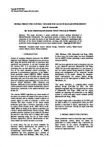
the control signal, Iup (p) values of the control signal applied to the plant at previous sampling instants and on nA + 1 values of the plant output signal measured at previous sampling instants. Unlike classical NARX predictions, they do not depend on predictions calculated for previous sampling instants within the prediction horizon. As a result, the multi-model is not used recurrently and the prediction error is not propagated. Figure 1 depicts the structure of the neural multi-model used for prediction in MPC. Arguments of the multi-model are chosen in such a way that predictions are independent of previous ones. The predictions yˆ(k + p|k) depend only on the future control policy and historical values of process variables. In general, arguments of the multi-model can be selected in a different way, e.g., as

(13)

where y(k) is measured while fp (k|k − 1) is calculated from the multi-model used for the sampling instant k: fp (k|k − 1) = fp (u(k − τ ), . . . , u(k − nB − p), (14) y(k − p), . . . , y(k − nA − p)).

3.2. Neural multi-model implementation. The multimodel is comprised of N MLP feedforward neural networks with one hidden layer and a linear output (Haykin, 1999). They realise the functions fp , p = 1, . . . , N , in (10). Outputs of the neural multi-model for the sampling instant k + p are y(k + p|k) =fp (x(k + p|k)) =w02,p +

Using (10) and (12), output predictions calculated from the multi-model are yˆ(k + p|k) =fp (u(k − τ + p|k), . . . , u(k|k),   

(15)

Iuf (p)

u(k − max(τ − p, 1)), . . . , u(k − nB ),    Iup (p)

y(k), . . . , y(k − nA ))    nA +1

+ d(k + p|k), where Iuf (p) = max(p − τ + 1, 0), Iup (p) = nB − max(τ − p, 1) + 1. Analogously as in the case of predictions (8) calculated from the classical NARX model (7), the predictions yˆ(k + p|k) calculated by means of the multi-model (10) depend on Iuf (p) future values of

(17)

p

K  i=1

wi2,p ϕ(zip (k + p|k)),

where zip (k + p|k) are sums of inputs of the i-th hidden node, ϕ : R −→ R is the nonlinear transfer function (e.g., hyperbolic tangent), K p is the number of hidden nodes. Recalling the prediction of the multi-model (15), one has zip (k + p|k) 1,p = wi,0 Iuf(p)

+

 j=1

1,p wi,j u(k − τ + 1 − j + p|k)

Iup(p)

+

 j=1

1,p wi,I u(k − max(τ − p, 1) + 1 − j) uf (p)+j

(18)

Nonlinear predictive control based on neural multi-models

11

Fig. 1. Structure of the neural multi-model used for prediction in MPC. nA+1

+

 j=1

which depends only on the past:

1,p wi,I y(k + 1 − j). uf (p)+Iup(p)+j 1,p wi,j ,

ˆ (k) = B(k)uN (k) + y 0 (k). y

(19)

p

Weights of networks are denoted by i = 1, . . . , K , j = 0, . . . , max(p−τ +1, 0)−max(τ −p, 1)+nA+nB +2, and wi2,p , i = 0, . . . , K p , for the first and the second layer, respectively, and p indicates the submodel, p = 1, . . . , N .

4. MPC algorithm with nonlinear prediction and linearisation based on neural multimodels If for prediction in MPC a nonlinear neural model is used without any simplifications, at each sampling instant the nonlinear optimisation problem (3) has to be solved on-line (Ławry´nczuk, 2007; Tatjewski, 2007). The difficulty of the resulting optimisation problem is twofold. First of all, it is nonlinear, computationally demanding, and its computational burden is high. Secondly, it may be non-convex and even multi-modal. Hence, a number of suboptimal MPC algorithms have been developed in which the neural model is linearised around the current operating point and the obtained linear approximation is next used for the optimisation of the future control policy (El Ghoumari and Tantau, 2005; Ławry´nczuk, 2007; 2008; 2009a; 2009b; Nørgaard et al., 2000; Tatjewski, 2007; Tatjewski and Ławry´nczuk, 2006). Thanks to linearisation, the future control policy is found by means of an easily solvable quadratic programming problem. In this paper the MPC algorithm with Nonlinear Prediction and Linearisation (MPC-NPL) (Ławry´nczuk, 2007; Tatjewski, 2007) is adopted to use neural multi-models.

Vectors of length N are T ˆ (k) = [ˆ y y (k + 1|k) . . . yˆ(k + N |k)] , T

uN (k) = [u(k|k) . . . u(k + N − 1|k)] ,  T y 0 (k) = y 0 (k + 1|k) . . . y 0 (k + N |k) .

(21) (22)

The matrix B(k) is calculated on-line from local linearisation of the neural multi-model: ⎡ ⎤ b1,0 (k) b1,1 (k) . . . b1,N −1 (k) ⎢ b2,0 (k) b2,1 (k) . . . b2,N −1 (k) ⎥ ⎢ ⎥ B(k) = ⎢ ⎥, .. .. .. .. ⎣ ⎦ . . . . bN,0 (k) bN,1 (k) . . . bN,N −1(k) (23) where the coefficients bp,l (k) =

x(k + p|k)) ∂fp (¯ , ∂u(k + l|k)

(24)

are calculated analytically for all p = 1, . . . , N , l = 0, . . . , N − 1, bp,l (k) = 0 for all p − τ + 1 ≤ l. The calculation of these quantities and of the nonlinear free trajectory depends on the model structure and is detailed in the following subsection. In MPC, only Nu ≤ N future control moves Δu(k) have to be found. Using the relation uN (k) = J Δu(k) + uk−1 N (k),   where J = JJ 12 is an N × Nu matrix, ⎡

4.1. MPC-NPL optimisation problem. In the MPCNPL algorithm at each sampling instant k the neural multi-model is used on-line twice: to find local linearisation and a nonlinear free trajectory. It is assumed that the ˆ (k) can be expressed as the sum output prediction vector y of a forced trajectory, which depends only on the future (on future control signals), and a free trajectory y 0 (k),

(20)

⎢ ⎢ J1 = ⎢ ⎣

1 0 1 1 .. .. . . 1 1

⎤ ... 0 ... 0 ⎥ ⎥ . ⎥ .. . .. ⎦ ... 1

(25)

(26)

is the all ones lower triangular Nu × Nu matrix, J 2 is the all ones (N − Nu ) × Nu matrix, and uk−1 N (k) =

M. Ławry´nczuk and P. Tatjewski

12 T

[u(k − 1) . . . u(k − 1)] is an N -dimensional vector, and the prediction equation (19) becomes 0 ˆ (k) = B(k)J Δu(k) + B(k)uk−1 y N (k) + y (k). (27)

Owing the superposition principle (27), in which it is assumed that future output predictions are linear functions of future input increments Δu(k), the general nonlinear MPC optimisation problem (3) becomes the following quadratic programming task:  min y ref (k) − B(k)J Δu(k) − B(k)uk−1 N (k) Δu(k)     2 2 −y0 (k)M + Δu(k)Λ , subject to umin ≤ J 1 Δu(k) + uk−1 (k) ≤ umax , −Δumax ≤ Δu(k) ≤ Δumax , 0 y min ≤ B(k)J Δu(k) + B(k)uk−1 N (k) + y (k) max ≤y ,

(28)

4.2. Algorithm implementation details. Linearisation points are vectors composed of past input and output signal values corresponding to arguments of consecutive submodels (10): ¯ (k + p|k) = [ u¯(k − 1) . . . u x ¯(k − 1)    Iuf (p)

u¯(k − max(τ − p, 1)) . . . u ¯(k − nB )    Iup (p)

y¯(k) . . . y¯(k − nA )]T ,    nA +1

for p = 1, . . . , N . The bar symbol over the process variables denotes values measured at previous sampling instants. Because future control signals are not known in advance, u ¯(k + p|k) = u ¯(k − 1) for p ≥ 0. Using a Taylor ¯ (k + p|k), linear approxiseries expansion at the points x mations of submodels, obtained at the sampling instant k, are y(k + p|k)

where

 T y ref (k) = y ref (k + 1|k) . . . y ref (k + N |k) , (29) T  (30) y min (k) = y min . . . y min ,

y

max

(36)

(k) = [y

max

...y

max T

u

= [u

max

...u

+

(32)

max T

(33)

] ,

Δumax = [Δumax . . . Δu

max T

T

uk−1 (k) = [u(k − 1) . . . u(k − 1)]

1. Linearisation of the neural multi-model: obtain the matrix B(k). 2. Find the nonlinear free trajectory y 0 (k) using the neural multi-model. 3. Solve the quadratic programming problem (28) to determine future control increments Δu(k). 4. Apply to the process the first element of the calculated vector Δu(k), i.e., u(k) = Δu(k|k)+u(k−1). 5. Set k := k + 1, go to Step 1.

x(k + For simplicity of presentation, bp,l (k) = bp,l (¯ p|k)). Taking into account the structure of the MLP neural multi-model given by (17) and (18), the coefficients of the linearised submodels are x(k + p|k)) ∂fp (¯ ∂u(k − l) ⎧ 0 if p − τ + 1 ≤ l, ⎪ ⎪ ⎪ Kp ⎪  ⎪ dϕ(zip (¯ x(k + p|k))) ⎨ wi2,p p = dzi (¯ x(k + p|k)) i=1 ⎪ ⎪ 1,p ⎪ ⎪ ·wi,p−τ +1−l ⎪ ⎩ if p − τ + 1 > l.

bp,l (k) =

(35)

are vectors of length Nu , and M = diag(μ1 , . . . , μN ), Λ = diag(λ0 , . . . , λNu −1 ). For simplicity of presentation, hard output constraints are used in (28). In practice, however, they are likely to lead to infeasibility problems. Hence, soft output constraints are recommended (Maciejowski, 2002; Tatjewski, 2007). All things considered, at each sampling instant k of the MPC-NPL algorithm the following steps are repeated:

bp,l (¯ x(k + p|k))(u(k + l) − u ¯(k − 1)). (37)

(34)

] ,

p−1  l=0

(31)

]

are N -dimensional vectors, T  umin = umin . . . umin , max

x(k + p|k)) = fp (¯

(38)

(39)

If a hyperbolic tangent is used as the nonlinear transfer function in the hidden layer of neural networks (i.e., ϕ = tanh), one has dϕ(zip (¯ x(k + p|k))) = 1 − tanh2 (zip (¯ xp (k + p|k))). dzip (¯ x(k + p|k)) (40) The nonlinear free trajectory y 0 (k + p|k), p = 1, . . . , N , is calculated on-line recurrently from the general prediction equation (12) using the neural multi-model defined by (17) and (18) and assuming no changes in the control signal from the sampling instant k onwards: p

0

y (k+p|k) =

w02,p +

K  wi2,p ϕ(zip,0 (k+p|k))+d(k+p|k). i=1

(41)

Nonlinear predictive control based on neural multi-models

13

The quantities zip,0 (k + p|k) are determined recurrently, in an analogous way as in (18), but assuming that u(k + p|k) = u(k − 1) for p ≥ 0: zip,0 (k + p|k) 1,p = wi,0 +

Iuf (p)

 j=1

Iup (p)

+



j=1 nA+1

+

 j=1

1,p wi,j u(k − 1)

1,p wi,I u(k − max(τ − p, 1) + 1 − j) uf (p)+j

Fig. 2. Polymerisation reactor control system structure. 1,p wi,I y(k + 1 − j). uf (p)+Iup (p)+j

(42) From (13) and (17), estimates of unmeasured disturbances are   Kp  2,p 2,p p d(k + p|k) = y(k) − w0 + wi ϕ(zi (k|k − 1)) , i=1

(43)

where, from (14) and (18), zip (k|k − 1) 1,p = wi,0 Iuf (p)

+

 j=1

1,p wi,j u(k − τ + 1 − j|k)

Iup (p)

+



j=1 nA+1

+

 j=1

1,p wi,I u(k − max(τ − p, 1) + 1 − j − p) uf (p)+j

1,p wi,I y(k + 1 − j − p). uf (p)+Iup (p)+j

(44)

5. Simulations 5.1. Polymerisation reactor control system. The process under consideration is a polymerisation reaction taking place in a jacketed continuous stirred tank reactor (Doyle et al., 1995) depicted in Fig. 2. The reaction is free-radical polymerisation of methyl methacrylate with azo-bis-isobutyronitrile as the initiator and toluene as the solvent. The output NAMW (Number Average Molecular Weight) [kg kmol−1 ] is controlled by manipulating the inlet initiator flow rate FI [m3 h−1 ]. The flow rate F [m3 h−1 ] of the monomer is a disturbance. Properties of the polymerisation reactor are nonlinear; it is frequently used as a benchmark for comparing nonlinear control strategies (Doyle et al., 1995; Ławry´nczuk, 2007; Tatjewski, 2007). The steady-state characteristic of the process is highly nonlinear, as shown in Fig. 3. As linear models cannot approximate the behaviour of the reactor, MPC algorithms

based on linear models are unable to control the process when changes in the reference trajectory are big and fast. Under some technological assumptions (Doyle et al., 1995), the continuous-time fundamental model of the polymerisation reactor is comprised of four nonlinear ordinary differential equations:    −EP dCm (t) = − ZP exp (45) dt RT   −Efm + Zfm exp Cm (t)P0 (t) RT F (t)Cm (t) F (t)Cmin + , − V  V −EI dCI (t) = − ZI exp (46) CI (t) dt RT F (t)CI (t) FI (t)CIin + , − V V   −ETc dD0 (t) = 0.5ZTc exp (47) dt RT   −ETd P02 (t) + ZTd exp RT   −Efm + Zfm exp Cm (t)P0 (t) RT F (t)D0 (t) , −   V  −EP dDI (t) =Mm ZP exp (48) dt RT   −Efm Cm (t)P0 (t) + Zfm exp RT F (t)DI (t) , − V where      P0 (t) =  

 2fIC (t)ZI

 ZTd exp

−EI RT



exp   , −ETd −ETc + ZTc exp RT RT (49)

M. Ławry´nczuk and P. Tatjewski

14

training the SSE performance index (9) is minimised in the case of the NARX model, while the SSE performance index (11) is minimised in the case of the multi-model. For each model, configuration training is repeated 10 times (the multi-start approach to nonlinear optimisation), and weights of neural networks are initialised randomly. The results presented next are the best ones obtained. Since input and output process variables have different orders of magnitude, they are scaled as u = 100(FI − FI0 ), y = 0.0001(NAMW − NAMW 0 ), where FI0 = 0.028328, NAMW 0 = 20000 correspond to the initial operating point. In all model types the hyperbolic tangent transfer function is used in hidden layers.

4

x 10 4.5

4

NAMW

3.5

3

2.5

2

1.5 0

0.01

0.02

0.03

0.04

0.05

0.06

F

I

Fig. 3. Steady-state characteristic of the reactor.

and the algebraic output equation is NAMW (t) =

DI (t) . D0 (t)

(50)

The initial operating conditions are FI = 0.028328 m3 h−1 , F = 1 m3 h−1 , NAMW = 20000 kg kmol−1 , Cm = 5.3745 kmol m−3 , CI = 2.2433 · 10−1 kmol m−3 , D0 = 3.1308 · 10−3 kmol m−3 , DI = 6.2616 · 10−1 kmol m−3 . Parameters of the model are given in Table 1. 5.2. Neural modelling of the polymerisation reactor. For the identification experiment the fundamental model (45)–(50) is used as the real process; it is simulated openloop in order to obtain two sets of data, namely, training and test data sets depicted in Fig. 4. Both sets contain 2000 samples, and the sampling time is 1.8 min. The output signal contains small measurement noise. During calculations the system of differential equations comprising the fundamental model is solved using the Runge-Kutta RK45 method. In the following part of the article, three model classes are compared: (a) a high-order classical NARX neural model, (b) a low order (underparameterised) classical NARX neural model, (c) a low-order (underparameterised) neural multimodel. Classical NARX models are trained non-recurrently (as one-step ahead predictors) and recurrently (as multiple-step ahead predictors), whereas the multi-model is trained only non-recurrently (recurrent training is not necessary). All neural models are trained using the BFGS optimisation algorithm (Bazaraa et al., 1993). During

5.2.1. High-order classical NARX neural model. In general, the accuracy of a model is determined by its order of dynamics and its approximation ability. Hence, if the order of dynamics is sufficiently high, the approximator is precise enough and the data set used for training is large enough, one may expect that the prediction of the classical NARX model is close to the actual response of the process. The following NARX neural model of order four (i.e., τ = 1, nA = nB = 4) is considered: y(k) = f (u(k − 1), u(k − 2), u(k − 3), u(k − 4), (51) y(k − 1), y(k − 2), y(k − 3), y(k − 4)). In the hidden layer, K = 10 hidden nodes are used. The number of training epochs is 200 (to avoid overfitting). The average training time is approximately 35 s and 125 s for non-recurrent and recurrent training, respectively (AMD Athlon 3.1 GHz). Table 2 compares the accuracy of the classical highorder NARX neural model trained non-recurrently and recurrently for both training and test data sets. The model is evaluated in two modes: non-recurrently and recurrently (values of performance indices SSEnon-recurrent and SSErecurrent). Naturally, the smallest value of SSErecurrent = 0.1636 (for the training data set) is obtained when the model is trained recurrently. When the model trained non-recurrently is used recurrently, SSErecurrent increases to 0.2866. In the light of the future application of the obtained high-order models in MPC, it is interesting to compare their long range prediction accuracy. Figure 5 shows the step-response of the process and long-range predictions. The prediction horizon N = 10 is used. Predictions are calculated recurrently by the classical highorder NARX neural model trained non-recurrently. The manipulated variable FI changes at the sampling instant k = 0 from 0.028328 to 0.004602, which corresponds to changing the operating point from NAMW = 20000 to NAMW = 40000. The step change does not belong to the training data set. Although the neural model is trained non-recurrently, it has very good long-range prediction

Nonlinear predictive control based on neural multi-models

15

Table 1. Parameters of the fundamental model.

Parameter

Value −3

8 kmol m 6 kmol/m−3 2.9442 · 103 kJ kmol−1 2.9442 · 103 kJ kmol−1 7.4478 · 104 kJ kmol−1 1.2550 · 105 kJ kmol−1 1.8283 · 104 kJ kmol−1 0.58 100.12 kg kmol−1

CIin Cmin ETc ETd Efm EI EP f∗ Mm

Parameter

Value

R T ZTc ZTd Zf m ZI ZP V

8.314 kJ kmol−1 K−1 335 K 3.8223 · 1010 m3 kmol−1 h−1 3.1457 · 1011 m3 kmol−1 h−1 1.0067 · 1015 m3 kmol−1 h−1 3.7920 · 1018 h−1 1.7700 · 109 m3 kmol−1 h−1 0.1 m3

Training data set

Test data set

0.04

0.04

F

F

I

0.06

I

0.06

0.02 0

0.02

1

500

1000

1500

0

2000

1

500

k

1500

2000

1500

2000

k

4

4

x 10

x 10

4

NAMW

NAMW

1000

3 2

4 3 2

1

500

1000

1500

2000

1

k

500

1000

k Fig. 4. Training and test data sets.

abilities. It correctly predicts the behaviour of the process over the whole prediction horizon. Figure 5 does not show predictions calculated recurrently by the model trained recurrently because they are much closer to the response of the process (in comparison with predictions calculated by the model trained non-recurrently). 5.2.2. Low-order classical NARX neural model. Irrespective of the training mode, the high-order NARX model has good long-range prediction abilities and can be used in MPC. In practice, however, the true order of dynamics is usually not known. Because, in fact, the fundamental model (45)–(50) consists of four differential equations, in order to precisely capture the nature of the process, the NARX model should have at least the second order, i.e., nA = nB = τ = 2 (Ławry´nczuk, 2007). The following low-order NARX model is considered (τ = nB = 2, nA = 1): y(k) = f (u(k − 2), y(k − 1)).

(52)

The model is intentionally underparameterised. One can expect that the low-order classical one-step ahead model (trained non-recurrently) has poor prediction abilities.

In the hidden layer, K = 6 hidden nodes are used. The number of training epochs is 200. The average training time is approximately 13 s and 27 s for non-recurrent and recurrent training, respectively. Table 3 compares the accuracy of the classical loworder NARX neural model trained non-recurrently and recurrently for both training and test data sets. The model is evaluated in two modes: non-recurrently and recurrently. It is worth noting that the low-order model has poor long-range prediction abilities in comparison with the high-order one (Table 2) (values of the performance index SSErecurrent are significantly bigger). Although for the low-order model recurrent training gives better longrange accuracy than non-recurrent training, properties of the obtained underparameterised model are rather poor when compared with the high-order structure.

5.2.3. Low-order neural multi-model. In order to finally show advantages of the multi-model approach (and disadvantages of the low-order classical NARX structure), the following multi-model (10) for N = 10 is considered:

M. Ławry´nczuk and P. Tatjewski

16

Table 2. Accuracy of the classical high-order NARX neural model trained non-recurrently and recurrently; the value of the SSE performance index actually minimised during training is given in bold.

Training data set SSEnon-recurrent SSErecurrent 0.2148 0.2866 0.2523 0.1636

Training mode Non-recurrent Recurrent

Test data set SSEnon-recurrent SSErecurrent 0.2412 0.6378 0.2574 0.2207

Table 3. Accuracy of the classical low-order (underparameterised) NARX neural model trained non-recurrently and recurrently, the value of the SSE performance index actually minimised during training is given in bold.

Training data set SSEnon-recurrent SSErecurrent

Training mode Non-recurrent Recurrent

0.3671 0.4841

2.7605 1.1189

4

x 10 3.2

3

NAMW

2.8

2.6

2.4

2.2

2 1

2

3

4

5

6

7

8

9

10

p Fig. 5. Step-response (long-range predictions) calculated by the classical high-order NARX neural model trained nonrecurrently (dashed line with circles) vs. the real process (solid line with points).

y(k + 1|k) =f1 (u(k − 1), u(k − 2),

(53)

y(k), y(k − 1)), .. . y(k + 10|k) =f10 (u(k + 8|k), . . . , u(k|k), u(k − 1), u(k − 2),

(54)

y(k), y(k − 1)). The multi-model is intentionally underparameterised in the same way as the low-order NARX model (52), and it has the same order of dynamics (τ = nB = 2, nA = 1). Submodels comprising the multi-model are trained as one-step ahead predictors (non-recurrently). The number of hidden nodes in submodels com-

Test data set SSEnon-recurrent SSErecurrent 0.5618 0.7805

7.5103 3.0351

prising the multi-model is adjusted in such a way that when trained and tested as one-step ahead predictors they give comparable values of the SSE performance index as the classical low-order (underparameterised) NARX model trained non-recurrently (Table 3). Naturally, for the multi-model the SSE index is calculated non-recurrently. Six submodels have K p = 3 hidden nodes (for p = 1, 6, 7, 8, 9, 10), four submodels have K p = 4 hidden nodes (for p = 2, 3, 4, 5). The number of training epochs is 200. The average training time varies from 7 s (submodel for p = 1) to 15.5 s (submodel for p = 10). For each sampling instant within the prediction horizon, one independent submodel is used. Therefore, the multi-model is not used recurrently in MPC. On the other hand, the total number of parameters (weights) of the rudimentary multi-model is big. In order to reduce the model complexity, the Optimal Brain Damage (OBD) pruning algorithm is used (LeCun et al., 1990). The accuracy of submodels (in terms of SSE) before and after pruning is shown in Fig. 6. The accuracy of the low-order underparameterised NARX model trained non-recurrently is marked with dashed lines (for both data sets). Pruned neural networks have good generalisation abilities although in the case of four submodels (p = 1, 3, 4, 6) the SSE performance index is slightly increased for the validation data set. For the training data set the accuracy of submodels is worse when compared with unpruned ones, but the deterioration is not significant. The complexity of submodels is reduced in the best case by 34.15% (submodel for p = 5), in the worst case by 17.65% (submodel for p = 6). An average complexity reduction factor is 29.66%. Figure 7 depicts the number of weights for all submodels before and after pruning. As both model types (i.e., the low-order NARX model and the multi-model) are trained as one-step ahead predictors, for the training data set, the values of the SSE index given in Fig. 6 refer to the one-step prediction error which is actually minimised during training. Analogously,

Nonlinear predictive control based on neural multi-models

17

Training data set

Test data set

0.9

0.9 Before pruning After pruning

0.7

0.7

0.6

0.6

0.5

0.5

0.4

0.4

0.3

0.3

0.2

0.2

0.1

0.1

0

1

2

3

Before pruning After pruning

0.8

SSE

SSE

0.8

4

5

6

7

8

9

0

10

1

2

3

4

5

p

6

7

8

9

10

p

Fig. 6. Accuracy of submodels p = 1, . . . , 10 before and after pruning for training (left) and test (right) data sets. The accuracy of the low-order underparameterised NARX model trained non-recurrently is denoted by dashed lines (for both data sets).

4

50

3.5

x 10

Non−recurrent training

45 40 3

Recurrent training

NAMW

N

w

35 30

2.5

25 20 15

2 10

1

2

3

4

5

6

7

8

9

10

p Fig. 7. Number of weights for submodels p = 1, . . . , 10 before (solid line) and after pruning (dashed line).

for the test data set models are also evaluated as one-step ahead predictors. When trained and tested as one-step ahead predictors both the low-order NARX model and the multi-model give comparable values of the SSE. It is an interesting question whether or not long-range prediction abilities of the multimodel are better than those of the NARX model. Figure 8 shows step-responses of the process and predictions. The manipulated variable FI changes at the sampling instant k = 0 from 0.028328 to 0.004602, analogously as in the experiment the result of which is shown in Fig. 5. The low-order NARX neural model is used recurrently, and it correctly calculates only the prediction for the first sampling instant of the prediction horizon (i.e., for p = 1). The model trained recurrently has better accuracy, but pre-

1

2

3

4

5

6

7

8

9

10

p Fig. 8. Step-responses (long-range predictions) calculated by the classical low-order (underparameterised) NARX neural model trained non-recurrently or recurrently (solid lines) and by the low-order underparameterised neural multi-model (dashed line with circles) vs. the real process (solid line with points).

dictions are still erroneous. As a result of underparameterisation, for next sampling instants the prediction error is propagated and consecutive predictions significantly differ from the real process. The neural multi-model is not used recurrently, and the prediction error is not propagated. In consequence, it has the ability to correctly predict the behaviour of the process over the whole prediction horizon. Differences between the process and predictions calculated from the multi-model are very small. In order to further compare long-range prediction accuracy and show the potential of using neural multimodels for long-range prediction in MPC, the following

M. Ławry´nczuk and P. Tatjewski

18 ratio is considered: RN =

N 1  N p=1



2

(y(k + p|k) − y(k + p)) k∈data set  . (yNARX (k + p|k) − y(k + p))2

k∈data set

(55) The coefficient RN compares average long-range prediction accuracy of the multi-model (numerator) and of the classical NARX model (denominator); both models are underparameterised. For the sampling instant k + p the output of the multi-model is denoted by y(k + p|k), the output of the classical NARX model used recurrently for long-range prediction is denoted by yNARX (k + p|k), and y(k + p) is the real data sample used for model training and testing. If RN < 1, it is clear that there is a potential for using multi-models, rather than classical NARX models in a recurrent way in MPC. The smaller the value of RN , the worse long-range prediction abilities of classical NARX models, and it is more appropriate to use multi-models in MPC. Calculated values of the ratio RN are given in Table 4. Two cases are considered: the NARX model is trained non-recurrently or recurrently. Unfortunately, for both training modes the model has poor accuracy in comparison with the multi-model. Although the multi-model is developed for N = 10, when evaluated, two prediction horizon cases are considered: N = 5 (for which R5 is calculated) and N = 10 (for which R10 is calculated). Because the prediction error is propagated, the longer the prediction horizon, the worse the prediction accuracy of the NARX model. 5.3. MPC of the polymerisation reactor. The fundamental model (45)–(50) is used as the real process during simulations of MPC algorithms. The model is solved using the Runge-Kutta RK45 method. The horizons of MPC are N = 10, Nu = 3, the weighting coefficients μp = 1, λp = 0.2. The following constraints are imposed on the manipulated variable: FImin = 0.003, FImax = 0.06. The sampling time of MPC is the same as the sampling time of neural models discussed in the previous subsection (1.8 min.). In MPC two underparameterised models are used, i.e., the low-order NARX structure and the low-order multi-model. They have the same order of dynamics (τ = nB = 2, nA = 1). Three MPC algorithms are compared: (a) the MPC algorithm with on-line Nonlinear Optimisation (MPC-NO) based on the low-order underparameterised NARX neural model, (b) the MPC-NO algorithm based on the low-order underparameterised neural multi-model, (c) the suboptimal MPC-NPL algorithm based on the same multi-model.

As the nonlinear optimisation routine in the MPC-NO algorithm, Sequential Quadratic Programming (SQP) (Bazaraa et al., 1993) is used on-line. The reference trajectory is ⎧ 20000 if k < 3, ⎪ ⎪ ⎪ ⎪ ⎨ 25000 if 3 ≤ k ≤ 19, 30000 if 20 ≤ k ≤ 39, (56) NAMW ref (k) = ⎪ ⎪ 35000 if 40 ≤ k ≤ 59, ⎪ ⎪ ⎩ 40000 if 60 ≤ k ≤ 80. 5.3.1. Control accuracy. Figure 9 depicts simulation results. In the MPC-NO algorithm based on the the loworder NARX neural model, the control policy is calculated on-line by means of nonlinear optimisation. Hence, it should be potentially very precise provided that the quality of the model used for prediction is high (and assuming that the optimisation procedure finds the optimal solution at each sampling instant). Unfortunately, long-range prediction accuracy of the low-order NARX model is poor in comparison with the multi-model (Fig. 8, Table 4). As a result, the MPC-NO algorithm based on the underparameterised NARX model used recurrently exhibits strong oscillatory behaviour. In contrast to that, both MPC-NO and MPC-NPL algorithms based on the same underparameterised multi-model are stable. Moreover, closedloop performance obtained in the suboptimal MPC-NPL algorithm with quadratic programming is very similar to that obtained in the computationally demanding MPC-NO approach, in which a nonlinear optimisation problem has to be solved on-line at each sampling instant. To make it possible to compare all three examined algorithms, the sum of squared differences between the reference trajectory and the actual value of the controlled variable over the whole simulation horizon, J=

k=80 

(NAMW ref (k) − NAMW (k))2 ,

(57)

k=1

is calculated after completing simulations. For the MPCNO algorithm based on the NARX model J = 5.3449 · 108 , for the MPC-NO algorithm based on the multi-model J = 3.9157 · 108 , and for the MPC-NPL algorithm based on the multi-model J = 3.9231 · 108 . 5.3.2. Computational complexity. Computational efficiency of the MPC-NPL algorithm is twofold. First of all, since the algorithm solves a quadratic programming problem, a unique global solution to the optimisation problem (28) is found at each sampling instant. Moreover, one may expect that the computational burden of the MPC-NPL algorithm is moderate in comparison with the MPC-NO approach. In order to verify this claim, the computational cost (in terms of floating point operations, MFLOPS) of both algorithms is calculated. They both

Nonlinear predictive control based on neural multi-models

19

Table 4. Average accuracy ratios RN : the multi-model in comparison with the classical low-order (underparameterised) NARX model trained non-recurrently or recurrently and used recurrently.

Data Training set Test set

Non-recurrent training R5 R10 0.4792 0.3581

Recurrent training R5 R10

0.3241 0.2298

0.3653 0.2911

0.2902 0.2271

4

x 10 4 3.8

0.025

3.6 3.4

F

I

NAMW

0.02

0.015

3.2

NAMWref

3 2.8 2.6

0.01

2.4 0.005

2.2 2 1

20

40

60

80

1

20

k

40

60

80

k

Fig. 9. Simulation results: the MPC-NO algorithm based on the low-order underparameterised NARX neural model (dotted line), the MPC-NO algorithm (solid line) and the MPC-NPL algorithm (dashed line) based on the same low-order underparameterised multi-model.

use the same neural multi-model. Next, the computational complexity reduction factor is calculated from computational cost of MPC-NO . F = computational cost of MPC-NPL

(58)

The factor F shows how many times the MPC-NPL algorithm is less computationally demanding in comparison with the MPC-NO scheme. Table 5 shows values of the factor F for different combinations of horizons (N = 5, 10, Nu = 1, 2, 3, 4, 5, 10). In general, the suboptimal MPC-NPL algorithm is many times computationally less demanding that the MPC-NO algorithm. 5.3.3. MPC based on parsimonious multi-models. Since in the multi-model the actual number of neural networks is equal to the prediction horizon, the total number of weights can be big. To reduce the number of parameters, the multi-model is pruned, which results in significant reduction of model complexity, as shown in Fig. 7. One can further reduce the number of parameters by considering only selected submodels, which corresponds to taking into account in the MPC cost function (2) only some differences between the reference trajectory and predictions. Good results are obtained when only five submodels are used. Submodels for p = 2, 4, 6, 8, 10 are used, and the weighting matrix in the MPC optimisation

task (28) is M = diag(0, 1, 0, 1, 0, 1, 0, 1, 0, 1).

(59)

Closed-loop performance of both algorithms is similar: for the MPC-NPL algorithm J = 3.8936 · 108 , for the MPC-NO algorithm J = 3.8534 · 108 (since the obtained simulation results are similar to those shown in Fig. 9, they are not given). These values are very close to those obtained when the multi-model comprised of ten submodels is used.

6. Conclusions Because MPC algorithms are very model-based, possible control performance is determined by the accuracy of the dynamic model. The role of the model in MPC cannot be ignored during model structure selection and identification. The model has to be able to make good predictions of future behaviour of the process over the whole prediction horizon. If neural models are trained non-recurrently using the rudimentary backpropagation algorithm, one-step ahead predictors are obtained. They are not suited to be used recurrently in MPC for long range prediction since the prediction error is propagated. This is important in the case of noise, model inaccuracies and underparameterisation. In particular, underparameterisation is potentially a

M. Ławry´nczuk and P. Tatjewski

20

Table 5. Computational complexity reduction factor F (the MPC-NO algorithm vs. the MPC-NPL algorithm based on the same neural multi-model).

N

Nu = 1

Nu = 2

Nu = 3

Nu = 4

Nu = 5

Nu = 10

5 10

5.83 8.69

7.49 12.83

9.04 14.67

9.81 15.19

10.27 13.56

− 12.21

very frequent source of prediction inaccuracies, as demonstrated in the paper. Usually, the order of models used in MPC is significantly lower than that of the real process, or the proper order is even unknown. In order to solve the problem resulting from the inaccuracy of one-step ahead predictors in MPC, the neural multi-model approach described in this paper can be efficiently used. The multi-model predicts future behaviour of the process over the prediction horizon without using previous predictions. It is demonstrated that low-order (underparameterised) neural models have poor prediction abilities, and recurrent training does not lead to any significant improvement. Conversely, the low-order neural multi-model (of the same order of dynamics) has good long-range prediction accuracy. The multi-model is trained easily using the classical backpropagation algorithm—no recurrent training algorithms are necessary. Intuitively, it is much easier to find independent submodels for consecutive sampling instants within the prediction horizon, rather than to train recurrently a single model of comparable long-range prediction accuracy. Although this paper describes the multi-model which is trained off-line and next used in the MPC-NPL algorithm, easy training is an important advantage when the multi-model is used in adaptive MPC (in which the model is trained on-line). An inherent feature of the multi-model is the fact that is has more parameters than classical NARX models of the same order of dynamics. Hence, it may be beneficial to prune submodels or take into account only some of them. Although MLP neural networks are used in this study, different types of networks can be considered, e.g., Radial Basis Functions (RBFs) (Ławry´nczuk, 2009a). In comparison with the structured neural model (Ławry´nczuk, 2009b), which is also designed with MPC in mind, the multi-model has an important advantage. The prediction horizon is not a parameter of the model—it only determines the number of submodels. Hence, changing the prediction horizon does not require retraining all submodels trained so far. When the horizon is lengthened, only lacking submodels must be trained. Conversely, when the horizon is shortened, no new models are necessary; some existing submodels are simply not used in MPC. The structured model is not so flexible—the prediction horizon is a parameter of the model and changing the horizon entails training the model. The presented suboptimal MPC-NPL algorithm cal-

culates on-line a linear approximation of the multi-model. Consequently, the future control policy is calculated by means of a numerically reliable quadratic programming procedure; the necessity of repeating full nonlinear optimisation at each sampling instant is avoided. In practice, the algorithm shows performance comparable to that obtained in MPC with nonlinear optimisation.

Acknowledgment The work presented in this paper was supported by the Polish national budget funds for science for the years 2009–2011 in the framework of a research project.

References ˚ Akesson, B. M. and Toivonen, H. T. (2006). A neural network model predictive controller, Journal of Process Control 16(3): 937–946. Alexandridis, A. and Sarimveis, H. (2005). Nonlinear adaptive model predictive control based on self-correcting neural network models, AIChE Journal 51(9): 2495–2506. Bazaraa, M. S., Sherali, J. and Shetty, K. (1993). Nonlinear Programming: Theory and Algorithms, John Wiley & Sons, New York, NY. da Cruz Meleiro, L. A., Jos´e, F., Zuben, V. and Filho, R. M. (2009). Constructive learning neural network applied to identification and control of a fuel-ethanol fermentation process, Engineering Applications of Artificial Intelligence 22(2): 201–215. Doyle, F. J., Ogunnaike, B. A. and Pearson, R. K. (1995). Nonlinear model-based control using second-order Volterra models, Automatica 31(5): 697–714. El Ghoumari, M. Y. and Tantau, H. J. (2005). Non-linear constrained MPC: Real-time implementation of greenhouse air temperature control, Computers and Electronics in Agriculture 49(3): 345–356. Greco, C., Menga, G., Mosca, E. and Zappa, G. (1984). Performance improvement of self tuning controllers by multistep horizons: The MUSMAR approach, Automatica 20(5): 681–700. Haykin, S. (1999). Neural Networks. A Comprehensive Foundation, 2nd Edition, Prentice-Hall, Englewood Cliffs, NJ. Henson, M. A. (1998). Nonlinear model predictive control: Current status and future directions, Computers and Chemical Engineering 23(2): 187–202.

Nonlinear predictive control based on neural multi-models Ławry´nczuk, M. (2007). A family of model predictive control algorithms with artificial neural networks, International Journal of Applied Mathematics and Computer Science 17(2): 217–232, DOI: 10.2478/v10006-007-0020-5. Ławry´nczuk, M. (2008). Suboptimal nonlinear predictive control with neural multi-models, in L. Rutkowski, R. Tadeusiewicz, L. A. Zadeh and J. Zurada (Eds), The 9th International Conference on Artificial Intelligence and Soft Computing, ICAISC 2008, Zakopane, Poland (Computational Intelligence: Methods and Applications), Exit, Warsaw, pp. 45–56. Ławry´nczuk, M. (2009a). Computationally efficient nonlinear predictive control based on RBF neural multi-models, in M. Kolehmainen, P. Toivanen and B. Beliczy´nski (Eds), The Ninth International Conference on Adaptive and Natural Computing Algorithms, ICANNGA 2009, Kuopio, Finland, Lecture Notes in Computer Science, Vol. 5495, Springer, Heidelberg, pp. 89–98. Ławry´nczuk, M. (2009b). Efficient nonlinear predictive control based on structured neural models, International Journal of Applied Mathematics and Computer Science 19(2): 233–246, DOI: 10.2478/v10006-009-0019-1. LeCun, Y., Denker, J. and Solla, S. (1990). Optimal brain damage, in D. Touretzky (Ed.), Advances of NIPS2, Morgan Kaufmann, San Mateo, CA, pp. 598–605. Liu, D., Shah, S. L. and Fisher, D. G. (1999). Multiple prediction models for long range predictive control, Proceedings of the IFAC World Congress, Beijing, China, (on CD–ROM). Lu, C. H. and Tsai, C. C. (2008). Adaptive predictive control with recurrent neural network for industrial processes: An application to temperature control of a variable-frequency oil-cooling machine, IEEE Transactions on Industrial Electronics 55(3): 1366–1375. Luyben, W. L. (1990). Process Modelling, Simulation and Control for Chemical Engineers, McGraw Hill, New York, NY. Maciejowski, J. M. (2002). Predictive Control with Constraints, Prentice Hall, Harlow. Morari, M. and Lee, J. (1999). Model predictive control: Past, present and future, Computers and Chemical Engineering 23(4): 667–682. Narendra, K. S. and Parthasarathy, K. (1990). Identification and control of dynamical systems using neural networks, IEEE Transactions on Neural Networks 1(1): 4–26. Nørgaard, M., Ravn, O., Poulsen, N. K. and Hansen, L. K. (2000). Neural Networks for Modelling and Control of Dynamic Systems, Springer, London. Parisini, T., Sanguineti, M. and Zoppoli, R. (1998). Nonlinear stabilization by receding-horizon neural regulators, International Journal of Control 70(3): 341–362. Pearson, R. K. (2003). Selecting nonlinear model structures for computer control, Journal of Process Control 13(1): 1–26. Peng, H., Yang, Z. J., Gui, W., Wu, M., Shioya, H. and Nakano, K. (2007). Nonlinear system modeling and robust predictive control based on RBF-ARX model, Engineering Applications of Artificial Intelligence 20(1): 1–9.

21 Qin, S. J. and Badgwell, T. (2003). A survey of industrial model predictive control technology, Control Engineering Practice 11(7): 733–764. Qin, S. Z., Su, H. T. and McAvoy, T. J. (1992). Comparison of four neural net learning methods for dynamic system identification, IEEE Transactions on Neural Networks 3(1): 122–130. Rossiter, J. A. and Kouvaritakis, B. (2001). Modelling and implicit modelling for predictive control, International Journal of Control 74(11): 1085–1095. Su, H. T. and McAvoy, T. J. (1992). Long-term predictions of chemical processes using recurrent neural networks: A parallel training approach, Industrial and Engineering Chemistry Research 31(5): 1338–1352. Tatjewski, P. (2007). Advanced Control of Industrial Processes, Structures and Algorithms, Springer, London. Tatjewski, P. and Ławry´nczuk, M. (2006). Soft computing in model-based predictive control, International Journal of Applied Mathematics and Computer Science 16(1): 101– 120. Temeng, K. O., Schnelle, P. D. and McAvoy, T. J. (1995). Model predictive control of an industrial packed bed reactor using neural networks, Journal of Process Control 5(1): 19–27. ´ Maciej Ławrynczuk was born in Warsaw, Poland, in 1972. He obtained his M.Sc. and Ph.D. degrees in automatic control from the Warsaw University of Technology, Poland, in 1998 and 2003, respectively. Currently, he is an assistant professor at the Institute of Control and Computation Engineering of the Warsaw University of Technology. His research interests include the application of neural networks in process modelling, control (particularly model predictive control) and set-point optimisation.

Piotr Tatjewski was born in Warsaw, Poland, in 1949. He received his M.Sc. (in electronic engineering), Ph.D. and D.Sc. degrees (in automatic control) from the Warsaw University of Technology in 1972, 1976 and 1988, respectively. Since 1972 he has been with the Institute of Control and Computation Engineering of the Warsaw University of Technology (1996–2008: the director of the Institute, 1993: a professor, 2006: a full professor). He is the author or a co-author of more than 30 journal papers, five books, including the recent Advanced Control of Industrial Processes. Structures and Algorithms (Springer, 2007) and Iterative Algorithms of Multilayer Optimizing Control (Imperial College Press/World Scientific, 2005, coauthored by M. A. Brdys). He is a member of the Committee on Automatic Control and Robotics of the Polish Academy of Sciences, and the EUCA (European Union Control Association). His current interests involve multilayer control, predictive control of linear and nonlinear processes, set-point optimisation, decomposition techniques in optimisation and control, and soft computing methods.

Received: 16 January 2009 Revised: 15 July 2009