Nonparametric Modeling of Vibration Signal Features for Equipment Health Monitoring Stephan W. Wegerich Al D. Wilks Robert M. Pipke SmartSignal Corporation 901 Warrenville Road Lisle, IL 60532 (630)-829-4000
[email protected]
Abstract—Monitoring of the vibration characteristics of mechanical systems provides valuable insight into the health of the equipment. Evaluation of vibration features using standards derived from performance of new systems provides benefits in numerous applications. Analysis of the data stream is carried out either on-line or off-line, often utilizing Fourier analysis techniques at a constant rate of operation. In many applications, acquiring vibration data only while the monitored machinery is operating at a specific condition is a difficult limitation that often results in a scarcity of useful data. To ideally assess the health of the machinery in a reliable and timely fashion, it is advantageous to monitor vibration at variable operating states thus avoiding many of the afore-mentioned data collection difficulties. In addition, it is possible to capture valuable machinery health information that might otherwise be neglected, since developing faults might be expected to appear preferentially at some of the different operating conditions.
constant and variable speeds. The features become the "sensors", analogous to the traditional sensors used in plant monitoring applications. We demonstrate an ability to reliably detect subtle changes in the modeled features within vibration data obtained from a laboratory mechanical test system with induced faults. These subtle changes can then be correlated with the severity of the induced faults, which in practice can provide a mechanism for estimating remaining useful life of the monitored machinery.
TABLE OF CONTENTS 1. INTRODUCTION .......................................1 2. NONPARAMETRIC MODELING ................2 3. TEST EQUIPMENT ...................................4 4. FAULT DETECTION SYSTEM (FDS) ........5 5. VIBRATION MONITORING WITH ECM ...6 6. CONCLUSION ...........................................9 REFERENCES ...............................................9
A nonparametric modeling technique developed by SmartSignal Corporation provides very early warnings of the onset of faults in plant applications over full operating ranges. A multivariate model is constructed based on traditional monitoring sensors (pressures, temperatures, flows, etc.); this model is then used to generate high fidelity real-time estimates of sensor values that represent normal plant behavior. These estimates are compared to the actual sensor readings to produce residuals that are analyzed to detect faulty system components. A variety of trending and statistical tests are used to reliably detect the evolving changes in the equipment. In doing so, the advantageous behavior of a residual constructed using a properly functioning model consistently facilitates early enunciation of the developing fault.
1. INTRODUCTION SmartSignal has developed an equipment condition monitoring product called eCM™ that has been used in a variety of monitoring applications in industries ranging from power generation to commercial airliners. The most common applications have relied on the existing low sampling rate monitoring sensors (like temperatures, pressures, levels, flows, etc) typically found on such systems. The eCM product employs at its core a purely data driven nonparametric modeling technology, that can be applied to any multivariate data stream in which a consistent relationship between individual streams exists (linear or non-linear). Thus, the modeling is generally applicable across wide ranges of applications. This paper first describes the nonparametric modeling approach broadly using available sensor data and then its application to fault
Here we demonstrate the use of this nonparametric approach for detecting faults in rotating machinery via extracted features from vibration signals captured at 0-7803-7651-X/03/$17.00 © 2003 IEEE
1
detection in rotating machinery using vibration signal features.
accelerometers and a tachometer. We first describe the nonparametric modeling approach employed by eCM in a general sense. Then the experimental setup of the MFS and the data collected from it are described. We then show the fault detection capabilities of eCM when applied to the vibration signal features extracted from the experimental data collected while the MFS is operated at both constant and variables speeds.
Monitoring rotating machinery using high frequency sensors like accelerometers to sense the operational state of the equipment offers significant diagnostic advantage over lower sample rate data collection approaches. It is well accepted that the vibration sensors provide the richest information source available for machine diagnosis in rotating systems. Unfortunately, the complexity of these signals and their variation with operational condition changes commonly found in such equipment makes the utilization of this information difficult.
2. NONPARAMETRIC MODELING The core of SmartSignal’s eCM software comprises a unique similarity based, nonparametric modeling technology referred to as the Signal Engine (SE). The SE generates estimates of the current values of each variable in a set modeled data sources. The data sources are typically sensor readings from sensors monitoring industrial equipment or processes. In contrast to 1st Principles modeling techniques, it is entirely empirical, i.e., data driven. The model is built from sets of “exemplars” or historic data observations that sufficiently characterize “normal” or “desirable” operation of the monitored equipment. In contrast to parametric modeling techniques (like polynomial regression or neural networks), no assumption about the form of the solution is imposed; the model is capable of making reasonable, if not exacting, estimates of proper equipment behavior globally by means of a localized weighted regression calculation. Another important feature of the SE is that any multivariate data stream can be modeled as long as there is some consistent relationship between individual streams (linear or nonlinear). Some examples of these are:
In a typical scheme the time domain signals acquired from these sensors are often transformed into the frequency domain where selected features of the spectral signals are used to identify signatures of specific fault scenarios [1]. To detect machinery faults, relevant features are usually monitored by simply comparing the magnitude of feature attributes to threshold values. If an attribute exceeds a specified level, the machinery is deemed faulty in some way. Due to the large a mount of variation that can be present in vibration spectra (especially when load and speed are changing), these threshold levels are typically set to be quite conservative to avoid false alerts. Unfortunately, this approach can lead to the detection of a fault when equipment damage is immanent, has already occurred or too late for any practical predictions of Useful Life Remaining (ULR). To avoid irreversible equipment damage and/or to effectively predict the ULR, one needs to (1) detect a fault early in its progression, (2) diagnose the fault, (3) measure the rate of degradation and (4) predict the severity of the fault (see [6], [7]). The eCM technology possesses properties that address all four of these issues [2]. These properties are: • • •
•
•
• • •
Capable of modeling highly variable systems; Multivariate, which facilitates the generation of multi-sensor/feature fault signatures Real-time algorithm with a small computational footprint allowing for real-time residual trending and pattern matching for diagnostics and prognostics Automatically adaptable to changing environmental conditions, which allows for the minimization of false alarms while still maintaining a high level of detection sensitivity Generally applicable (universal modeler), which means that any multivariate data source can be modeled as long as there are meaningful relationships within the data
•
Process variables such as pressure, temperature, flow Vibration signal spectral components Wavelet transform coefficients calculated from transient data Statistical values of time series data such as the mean, variance, skewness and kurtosis
In each of these cases, the data streams are composed of selected relevant features, which act as monitoring "sensors" akin to the pressures, temperatures, and flows used in many traditional monitoring schemes. The primary requirements of the technology are: 1. 2.
Good historic data truly representing the equipment free from fault, and Sufficient historic data to properly encompass the patterns of interaction among the variables
Both of these requirements are hallmarks of all empirical techniques. However, SmartSignal has developed tools for data cleansing to address requirement (1), and adaptive bootstrapping techniques for implementations where
In this paper we apply the eCM approach to vibration signals monitoring a SpectraQuest, Machinery Fault Simulator (MFS) which is comprised of a variable speed motor driving a loaded shaft and is outfitted with four 2
sufficient data is not available at first to address requirement (2).
contributors to the estimate of the input vector Yin. In the extreme case, when Yin exactly equals one of the vectors contained in D, Yest = Yin meaning that the weights in w are all 0 except for the one that corresponds to the like vector. The similarity operator for use in the above meets the following criteria:
The SE technology is based on the application of a “similarity operation” on pairs of observation vectors and the manipulation of a "state" matrix (D) containing the historical data exemplars described above. Thus, the state matrix will have its number of columns equal to the number of representative exemplars (M) and its number of rows equal to the number of data sources contained in each exemplar (L). Defining the set of measurements taken at a given time nj as an exemplar vector, Y(nj),
[
Y (n j ) = y1 (n j ) y2 (n j ) y3 (n j ) K yL (n j )
]
1. 2. 3.
t
(1)
The similarity operation can be a vector operation or can be an element-to-element operation that is averaged across the vectors being compared. For example, one vector-to-vector similarity operation that can be used is based on the Euclidean distance in N-space (where N is the number of data sources in the observation):
where yi(nj) is the measurement from data source i at time nj, then the state matrix D is given by:
D = [Y (n1 ) Y (n2 ) Y (n3 ) K Y (nM )]
(2)
⎧⎪ S ( x, y) = ⎨1 + ⎪⎩
The result of the similarity operation is a similarity score (a scalar) for the comparison of the two observation vectors. The similarity operation is akin to the dot product, and can be extended to matrix operations (although it is non-linear), where a scalar similarity score is rendered for each combination of a row from one matrix and column from a second matrix. Accordingly, given an input vector Yin containing single readings from each of the L data sources, a vector of corresponding estimated data source values, Yest, is determined from [2-5]: Y est = D ⋅ w . (3) The estimate is composed of a linear combination of the exemplars stored in D. Here, w is a weighting vector derived from: wˆ (4) w= ⎛ N ⎞ ⎜ ∑ wˆ ( j ) ⎟ ⎜ ⎟ ⎝ j =1 ⎠
(
wˆ = Dt ⊗ D
) ⋅ (D ⊗ Y ) = G −1
t
in
−1
⋅A
2.
⎫⎪ ( x(n) − y (n)) ⎬ ∑ ⎪⎭ n =1 N
−1
2
(6)
An example of an element-to-element similarity operation that can be used is:
1 S ( x, y ) = N
⎧ x ( n) − y ( n) ⎪ ⎨1 + ∑ R ( n) n =1 ⎪ ⎩ N
⎫ ⎪ ⎬ ⎪⎭
−1
(7)
The D matrix of exemplars is typically created from a large set of historic reference data covering the full dynamic range of the monitored equipment. The selection of exemplars is accomplished such that a minimal number of vectors represent the full range of equipment operation. SmartSignal has developed a number of proprietary techniques for this. All such selection steps are one-pass processes, in contrast to iterative training algorithms that characterize parametric approaches like neural networks. Consequently, they are both extremely fast as well as deterministic. The number of exemplars required is dependent on both the number of sensors in the model, as well as the dynamic variability of the equipment in normal operation. However, a general rule of thumb provides for the selection of a number of exemplars no less than 2 times the number of sensors. It is not uncommon to model a 5060 sensor system with 200-300 exemplars.
(5)
The similarity operation is indicated by the symbol ⊗ (which is not here meant to designate the Kronecker Product as it is sometimes used in literature). Equation (5) can be interpreted as a two-step transformation: 1.
Similarity is a scalar range, bounded at each end The similarity of two identical inputs is the value of one of the bounded ends The absolute value of the similarity increases as the two inputs approach identity
Measure the amount of similarity between the input vector and each of the corresponding exemplars to produce a similarity score vector, A Transform (premultiply by G-1) the score vector into a set of weighting factors that are then used to compose an estimate based on a linear combination of the exemplars in D.
Multiplying through by G-1 has the effect of increasing or decreasing the number of vectors in D that are significant 3
Figure 1 - Estimate of a Point on an Unknown Surface
Figure 2 - Experimental Machinery Fault Simulator
As can be seen in Figure 1, an unknown dynamics surface is empirically mapped by exemplars (shown in blue), using the SmartSignal modeling technology. An estimate (shown in red) is generated as a weighted combination of the exemplars. The contributions (as shown in green along each contributing exemplar) can be both positive and negative. In the classic inferential mode common to most modeling approaches, where estimates are made for variables that are not in the input vector, the D matrix comprises two subsets, one of input exemplars, and one of corresponding output exemplars. Equations 3 and 5 above become:
The vertically mounted accelerometer on the bearing housing nearest to the motor is used in this study. The accelerometer signal is first filtered using an anti-aliasing filter with a cutoff frequency of ~9 kHz. Then the filtered signal is digitized via a 12-bit DAQ system with a sampling rate of 20 kS/s. An overview of the experimental system is shown in the block diagram of Figure 3.
(
Y est = Dout ⋅ w
wˆ = Dint ⊗ Din
) ⋅ (D −1
t in
The MFS allows one to simulate faults in a variety of ways. Here we focus on a shaft imbalance fault and two types of bearing faults. The shaft imbalance fault case is induced by attaching a weight (a small bolt) to the outer radius of one of the loading discs (see Figure 2). The bearing faults are simulated using a set of bearings each containing a different type of fault. Three sets of bearings are used: a completely normal bearing; a bearing containing a single faulty ball; and a bearing with a faulty outer race. Inserting a single, small notch on the surface of the specific bearing component creates the fault. SpectraQuest supplied all faulted bearings used in this study. Data used to produce the experimental results in this paper were collected while operating the MFS at variable speeds from 0 to ~25 rev/s. The speed was systematically varied while data were collected over a 25 second period. A minimum of two data sets was collected while the MFS operated normally and while operating with each of the faults present. One of two normal data sets was used to build a nonparametric model for the imbalance fault case and one of three normal data sets was used to generate the model for the both of the bearing fault cases. These models were then used to drive the SE component of the fault detection system described in the following section.
(3a)
⊗ Y in
)
(5a)
Advantageously, the modeling technique is also capable of generating estimates in what we call the “autoassociative” mode, where all outputs are also inputs (equations 1 and 3 above). This is a critical advantage (and somewhat unorthodox in the modeling world) for the common situation where the instrumented variables of the equipment represent a mix of the causes and effects of the physics that drive the equipment. It ameliorates the need to determine causes and effects and feedback, and reduces the “illposedness” caused by many-to-one state issues.
3. TEST EQUIPMENT To explore the feasibility of applying the eCM Signal Engine (SE) to vibration monitoring for equipment health monitoring, a SpectraQuest variable speed Machinery Fault Simulator (MSF) was used to generate normal operation data and fault data. The simulator (pictured in Figure 2) is comprised of a ½ HP variable speed motor driving a shaft– rotor component supported with two sets of bearings. The MSF is outfitted with 4 accelerometers and a tachometer, which are all connected to a National Instruments, PCbased, DAQ system.
4
Figure 4 – Fault Detection System (FDS) Flow Diagram. A Hanning window is applied to a fixed-size window of vibration data and then the windowed data are transformed into the frequency domain using the FFT. The Power Spectral Density (PSD) is then calculated from the window of transformed data. The window is then moved to include 75% of the most recent samples from the previous window and 25% of the samples from newly acquired samples. The PSD calculation is repeated and the process continues throughout each vibration data set. Once the feature extraction process is applied to one of the normal data sets, the exemplars used to define the state matrix (D) can be selected. Creating the D matrix essentially completes the modeling process and enables the SE to be used to calculate estimates of incoming feature vectors. Residual vectors are created by subtracting the estimate vector from the input feature vector which results in a signature that can be used to identify faults and/or equipment operation deviating from normal behavior (normal behavior represented by the exemplars used to create D). Residual patterns (or signatures) are analyzed using a variety of techniques. These include:
Figure 3 – System Overview
4. FAULT DETECTION SYSTEM (FDS) Traditionally the SE component of eCM operates on raw sensor data acquired from common low frequency monitoring sensors such as thermocouples, pressure transducers and flow meters. The SE is inherently multivariate and therefore requires multiple data streams to operate properly. To monitor a single sensor (like an accelerometer) it is therefore necessary to extract multiple features from the sensor signal to produce the multivariate data stream. There are many ways to accomplish this result depending on the application at hand. Examples of some of the approaches include: • • •
•
• •
The frequency components of a Short Time Fourier Transform (STFT) Coefficients of the of the Discrete Wavelet Transform (DWT) Statistical measurements that characterize a time series (mean, standard deviation, skewness, kurtosis, crest factor, RMS, etc.)
Applying a hypothesis test (the Sequential Probability Ratio Test (SPRT) for example) to each feature over time to produce alerting patterns which can be matched with stored alerting patterns Classifying time-frequency patterns of raw or thresholded residuals using a similarity operator like those defined in equations 6 and 7 Simple visual interpretation by taking advantage of the filtering characteristics resulting from applying the modeling engine
In any case, having the residual patterns themselves facilitates the diagnosis of faults by enhancing those features that deviate from the normal behavior of the monitored equipment and suppressing those that are common with normal behavior. This trait is especially advantageous for vibration monitoring since vibration signals tend to be extremely complex and information rich even during normal equipment operation. Operating at variables speeds and loads only adds to the complexity. In the next section we demonstrate the feasibility of applying the FDS to detect faults by monitoring vibration signals. Of
A flow diagram of the Fault Detection System (FDS) used to analyze vibration signals is shown in Figure 5. The raw vibration signal is fed into a feature extraction module that provides the multivariate data for the SE module. The Short Time Fourier Transform (STFT) is employed as the signal decomposition methodology for generating the features. 5
particular interest is the fact that the results are all generated from monitoring data acquired while the MSF is operating at variable speeds.
the SE for the normal operation case. The bottom plot shows the residual generated by subtracting the estimate of the spectral signal from the actual spectral signal.
5. VIBRATION MONITORING WITH eCM The feasibility of applying eCM to vibration monitoring applications is illustrated in the following results. The study is carried in two phases, one in which the focus is on detecting a shaft imbalance and one where the focus is on detecting two types of bearing faults. In each case, the residual patterns produced by the FDS are used as the indication of either normal equipment operation or operation in the presence of one of the induced faults. In both phases a particular frequency range is used to do the modeling. All frequency components are used within the identified range to determine if it is feasible to simply model all components whether relevant or not. Phase 1: Shaft Imbalance The frequency range necessary for the FDS to detect a shaft imbalance is 5 to 100 Hz. The FFT size used to calculate the features is 4096 at 5 kS/s resulting in a frequency resolution of ~1.2 Hz/sample (the data are actually acquired at 20 kS/s but are down-sampled in this case to increase the low frequency resolution.) Two sets of data were collected that represent normal operation, each acquired for 25 seconds resulting in 500,000 time domain samples. The STFT is applied to the time domain data to produce the modeling features used in the FDS. 300 exemplars were selected from the full set of spectral data to generate the D matrix making it 78 rows by 300 columns, since the number of features represented in the spectral signal from 5 to 100 Hz is 78.
Figure 6 – Modeling at t=18.4 s (normal)
Figure 7 – Modeling at t=24.1 s (normal) As the speed is increased, the spectral components shift to the right as expected. The model follows the variation in the spectral components causing all of the residual components to hover around zero, which indicates normal operating conditions. The same spectral time instances are shown in figures 8, 9 and 10, however in this case an imbalance is present.
Figure 5 – Modeling at t=14.3 s (normal) Figures 5, 6 and 7 show, in the top plots, the spectral signals calculated using the Short Time Fourier Transform (STFT) at three different instances in time along with the corresponding estimate of the spectral signal generated by 6
The model follows many of the components, however the fundamental frequency and some of the fundamental harmonics show a large discrepancy even as the motor speed increases. This deviation is clearly visible in the corresponding residual plots. The residual essentially filters out all of the extraneous information leaving only the important indicators of the presence of a shaft imbalance. Importantly, the signature of this fault is expected to scale with the square of shaft speed, but the SE has encoded that relationship in its family of exemplars, which allow one to see useful information over a wide speed range when using this technique coupled with the SE. Hence, this residual is informative as a signature for this particular fault mode at multiple speeds. This is further illustrated in Figure 11. The top two plots show the spectrograms of the raw data with and without the presence of an imbalance. In both cases, there are many strong frequency components (red indicates large amplitudes and blue indicates small amplitudes) present over time and frequency making it somewhat difficult to detect the imbalance. However, plotting the residual signals in analogous time-frequency intensity plots clearly shows the absence and presence of the imbalance. Here, the time-frequency residual plot serves as a fault "picture" used to identify and distinguish multiple failure types.
Figure 8 – Modeling at t=14.3 s (imbalance)
Figure 9 – Modeling at t=18.4 s (imbalance)
Figure 11 – Spectrograms and Time-Frequency Residuals (imbalance fault) Figure 10 – Modeling at t=24.1 s (imbalance) Phase II: Bearing Faults 7
In the case of the bearing faults, the modeling was extended to include frequency components ranging from 5 to 700 Hz. This is due to the presence of significant higher order harmonic frequency components that are indictors of the bearing faults. The data are not down-sampled to increase the lower end resolution and therefore retain the 20 kS/s sample rate. Because of this, the frequency resolution is lowered to 4.88 Hz/sample. The number of features modeled is now 142, however the number of exemplars is kept constant at 300 for a final D size of 142 rows by 300 columns.
over time and frequency making it difficult to detect the fault. However, plotting the residual signals in analogous time-frequency intensity plots clearly show the presence of the fault. The type of fault can be interpreted by measuring the spacing between the bands in the residual plot as time increases. In this case, the spacing amounts are consistent with a ball fault, which for this bearing has a fundamental frequency of about 18 Hz at 10 rev/s and 37 Hz at a 20 rev/s which is the range of operating speeds used in the experiments.
As in the imbalance case, the residual filters out all of the extraneous information leaving only the important indicators of the presence of a fault. The plots in Figure 12 show the response of the SE to a bearing containing a ball fault. The top two plots are the spectrograms of the raw data with and without the presence of an imbalance. The normal spectrogram is on the left and the spectrogram with the fault is on the right.
Figure 13 - Spectrograms and Time-Frequency Residuals (outer race fault) The analogous plots shown in Figure 13 demonstrate the SE performance when an outer race bearing fault is present in the MFS. Once again, the normal time-frequency residual plot (bottom left) is absent of any structure, meaning that all elements in the residual pattern are close to zero. The raw spectrograms contain vast amounts of spectral information. It would be difficult in the normal case to decide whether or not a fault exists. However, since the SE closely estimates all of the spectral data over time, none of the frequency components stand out (residual pattern shows no structure). In contrast, the fault case plots clearly show the presence of the fault. The residual pattern emphasizes those components that are related to the outer race fault and suppresses the rest. The frequency spacings of the emphasized components range from about 30 Hz to 80 Hz. This is consistent with the expected harmonic spacings calculated for this bearing with an outer race fault operating
Figure 12 - Spectrograms and Time-Frequency Residuals (ball fault) The changing speed of the MFS is indicated by the spectral bands moving towards the right (increasing frequency) and then back to the left (decreasing frequency) over time. Again, in both the normal and fault cases, there are many strong frequency components (red indicates large amplitudes and yellow indicates small amplitudes) present 8
at speeds ranging from about 10 to 25 rev/s, which is how the experiment was performed.
the 9th International Conference on Intelligent Systems Applications to Power Systems, July 6-10, 1997.
6. CONCLUSION
[6] C. Talbott, "Diagnostics and Prognosis of Large Horsepower Electric Submersible Pumps," 13th International Congress, Condition Monitoring and Diagnostic Engineering Management, December 2000.
Providing effective predictions of Useful Life Remaining requires the basic steps of detecting a fault early in its progression, diagnosing the fault, and measuring its rate of degradation and/or severity. In the world of vibration monitoring, providing this information is often complicated due to the complexities of physical interactions in mechanical systems that manifest themselves in vibration signals. These matters are further complicated when the requirement is to monitor equipment continuously while operating over a wide range of states. We have shown that the eCM technology developed at SmartSignal possesses properties that can overcome these obstacles by acting as an extraneous information filter. Having the ability to compare a feature set to a modeled feature set over all operating conditions enables the identification of particular fault modes earlier in their progression. In addition, the magnitudes of the components of the residual patterns produced by eCM are related to the severity of the fault, which is useful for predicting ULR in machinery. In future work we will attempt to makes this connection more clear. Also, because the SE component of eCM is capable of handling many different data sources, it is possible that combining features such as those from vibration data with more tradition monitoring data (pressures, temperatures, flows, etc.) could provide a further enhancement in the ability to detect, diagnose and prognosticate faults. The authors plan to continue to expand the capabilities of the eCM technology in the vibration monitoring space.
[7] J. Gertler, Fault Detection and Diagnosis in Engineering Systems, Marcel Dekker, Inc. New York, 1998.
Stephan Wegerich joined SmartSignal in 1999 after 6 years at Argonne National Laboratory. While at Argonne, he worked on signal processing applications and the multivariate state estimation technique (MSET), which is the precursor to eCM. He is a recipient of the 1998 RD-100 award for his contributions to the development of MSET. He is a specialist in signal processing, and has 11 patents issued and has an extensive list of publications and presentations. He holds BS in Electrical Engineering from Southern Illinois University and a MS in Electrical Engineering and Computer Science from the University of Illinois at Chicago. Alan Wilks co-founded SmartSignal after over 30 years of industrial research experience. During a 26year career at AlliedSignal (where he held the position of VP of Research and Technology), he directed and managed research programs for a broad slate of very diverse businesses, including UOP, Bendix, Garrett, Norplex, Autolite and others. He holds 7 US patents and has numerous publications and presentations. He is an Analytical Chemist holding a BS from the University of Kansas and a PhD from the State University of Iowa.
REFERENCES [1] V. Wowk, Machinery Vibration, Measurement and Analysis, McGraw-Hill, Inc., Boston Massachusetts, 1991. [2] S. Wegerich, R. Singer, J. Herzog, and A. Wilks, "Challenges Facing Equipment Condition Monitoring Systems," Maintenance and Reliability Conference Proceedings, May 2001. [3] J. Mott, R. Young, and R. King, "Pattern-Recognition Software for Plant Surveillance," Proeedings of the International Meeting on Nuclear Power Plant Operation, August 30-September 3, 1987.
Matt Pipke came to SmartSignal as a former principal at Technology Solutions Company, a business-tobusiness IT consulting firm. He was previously an intellectual property attorney with the law firm of Fitch, Even, Tabin and Flannery in Chicago. In addition, he served as president and cofounder of Western Algorithmic Corporation, a software and networking firm. He has a JD from Loyola University of Chicago, and a BA in Physics from the University of Chicago.
[4] J. Mott, R. King, and W. Radtke, "A Generalized System State Analyzer for Plant Surveillance," Artificial Intelligence and Other Innovative Computer Applications in the Nuclear Industry, M. Majumdar, et. al. eds., Plenum Press, New York, 1988. [5] S. Singer, K. Gross, J. Herzog, S. Wegerich, and W. King, "Model-Based Nuclear Power Plant Monitoring and Fault Detection: Theoretical Foundations," Proceedings of 9