Psychonomic Bulletin & Review 2009, 16 (6), 1129-1135 doi:10.3758/PBR.16.6.1129
Notes and Comment
The overconstraint of response time models: Rethinking the scaling problem Chris Donkin, Scott D. Brown, and Andrew Heathcote University of Newcastle, Callaghan, New South Wales, Australia
Theories of choice response time (RT) provide insight into the psychological underpinnings of simple decisions. Evidence accumulation (or sequential sampling) models are the most successful theories of choice RT. These models all have the same “scaling” property—that a subset of their parameters can be multiplied by the same amount without changing their predictions. This property means that a single parameter must be fixed to allow the estimation of the remaining parameters. In the present article, we show that the traditional solution to this problem has overconstrained these models, unnecessarily restricting their ability to account for data and making implicit—and therefore unexamined—psychological assumptions. We show that versions of these models that address the scaling problem in a minimal way can provide a better description of data than can their overconstrained counterparts, even when increased model complexity is taken into account.
Many psychological experiments involve a choice between two alternatives. Despite their apparent simplicity, there are many complicated empirical regularities associated with the speed and accuracy of such choices. Response time (RT) distributions take on characteristic shapes that differ systematically, depending on whether the associated response is correct or incorrect, and depending on any number of experimental manipulations of stimulus properties or of instructions to the participants. A range of theories have been proposed to account for both choice probability and RT when making simple decisions (for reviews, see Luce, 1986; Ratcliff & Smith, 2004). Over the past 40 years, evidence accumulation (or “sequential sampling”) models have dominated the debate about the cognitive processes underlying simple decisions (see, e.g., Busemeyer & Townsend, 1993; Ratcliff, 1978, Ratcliff & Smith, 2004; Smith, 1995; Stone, 1960; Usher & McClelland, 2001; Van Zandt, Colonius, & Proctor, 2000). More recently, evidence accumulation models have been applied more widely, for example, as general tools to measure cognition in the manner of psychometrics (Schmiedek, Oberauer, Wilhelm, Süß, & Wittmann, 2007; Vandekerckhove, Tuerlinckx, & Lee, 2009; Wagenmakers, van der Maas, & Grasman, 2007), and as models for the neurophysiology of simple decisions (see, e.g., Forstmann et al., 2008; Ho, Brown, & Serences, 2009; Smith & Rat-
cliff, 2004). In light of this growing influence, it is especially important that users of these models are not misled by implicit—and hence unexamined—assumptions. Evidence accumulation models all share a basic framework wherein, when making a decision, people repeatedly sample evidence from the stimulus. This evidence is accumulated until a threshold amount is reached, which triggers a decision response. These models naturally predict the response made (depending on which response has accumulated the most evidence) and the latency of the response (depending on how long the evidence took to accumulate). We illustrate these models using the example of a lexical decision task, in which a participant must decide whether a string of letters is a valid word (e.g., dog) or not (e.g., dxg). The participant samples information from the stimulus repeatedly and finds some evidence that suggests that the stimulus is a word, and other evidence to suggest that the stimulus is not a word. The participant accrues this information, waiting until there is enough evidence for one of the two options before responding. His or her choice corresponds to the response with the most evidence, and the time taken for this evidence to be accumulated is the response latency. Over the past four or five decades, dozens of evidence accumulation models have been proposed, and all of them share a mathematical “scaling property”: One can multiply a subset of their parameters by an arbitrary amount, without changing any of the model’s predictions. To avoid complications arising from the scaling property, just one parameter of the model must be constrained arbitrarily. We show that the conventional approaches—which have been universally applied to solve the scaling problem—have actually overconstrained the models by fixing more than one parameter. This overconstraint has been largely unrecognized by the field, so it is equivalent to making a tacit, untested, psychological assumption. Furthermore, we show that this tacit assumption can sometimes have important consequences: When the scaling problem is solved in a minimal way, the models can sometimes provide a better account for data. Overview of the Models There are two major classes of evidence accumulation models: single accumulator models (Busemeyer & Townsend, 1993; Ratcliff, 1978; Ratcliff & Rouder, 1998; Ratcliff & Tuerlinckx, 2002; Smith, 1995; Stone, 1960) and models that have one accumulator for each possible response (Brown & Heathcote, 2005, 2008; Smith & Van Zandt, 2000; Smith & Vickers, 1988; Townsend & Ashby, 1983; Usher & McClelland, 2001; Van Zandt et al., 2000; Vickers, 1970). The customary method for solving the scaling problem differs between the two classes of models, even though the principle is the same. To simplify our dis-
C. Donkin,
[email protected]
1129
© 2009 The Psychonomic Society, Inc.
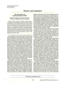
1130 Donkin, Brown, and Heathcote cussion, we choose a specific model from each class: the single accumulator diffusion model (Ratcliff & Tuerlinckx, 2002) and the multiple accumulator linear ballistic model (LBA; Brown & Heathcote, 2008). We have chosen these two models largely for convenience, since both have easyto-implement computer code that is freely available (see Donkin, Averell, Brown, & Heathcote, 2009, and Voss & Voss, 2007). The general point that we make, however, applies to all evidence accumulation models. Continuing the lexical decision example, the diffusion model assumes that participants sample evidence from the stimulus continuously, and that evidence stream updates an evidence total, say, x, illustrated as a function of time by the irregular line in Figure 1. The accumulator begins the decision process in some intermediate state, say, x 5 z. Evidence that favors the response “word” decreases the value of x, and evidence that favors the other response (“nonword”) increases the value of x. The evidence accumulation process continues until sufficient evidence favors one response over the other, causing the total (x) to reach one of its two boundaries (the horizontal lines at x 5 0 and x 5 a in Figure 1). The choice made by the model depends on which boundary is reached (a for a nonword response or 0 for a word response), and the RT equals the accumulation time plus a constant, Ter , that represents the time taken by nondecision processes, such as encoding the stimulus and producing the response. Depending on the stimulus, evidence tends to accumulate more toward one boundary or another, and the average rate of this accumulation is called the “drift rate,” which we will label v. The evidence accumulation process also varies randomly from moment to moment during the accumulation process, and the amount of this variability is another parameter of the model, s. Recent applications of the diffusion model include three extra parameters, but
these are not important for our purposes, so we will delay their introduction until later. When experimental conditions differ only in stimulus characteristics that vary randomly from trial to trial, all parameters except the drift rate are conventionally assumed constant over conditions (Ratcliff, Gomez, & McKoon, 2004). The LBA is a multiple accumulator model, meaning that it assigns a separate evidence accumulator to each possible response: For example, in lexical decision, one accumulator gathers evidence in favor of the word response, and the other gathers evidence for the nonword response, as is illustrated in Figure 1. The activity level in each accumulator begins at a value that is randomly sampled (separately for each accumulator) from the interval [0, A]. Evidence accumulation is noiseless (“ballistic”) and linear, with a slope that we again call the “drift rate,” v. When the evidence accumulated for either response reaches a threshold, b, a response is made. Like the diffusion model, the LBA assumes that nondecision processing takes fixed time, Ter . The drift rates are assumed to vary from trial to trial according to normal distributions, with means v W for the word accumulator and vNW for the nonword accumulator, and a common standard deviation, s. Scaling Properties Consider just one of the evidence accumulators from the LBA. The accumulator begins a trial with some activity, say x0, between 0 and A, and increases at a rate of v units/sec (v is the drift rate for this accumulator). Evidence accumulation ends when the threshold b is reached, which will take (b2x0)/v seconds. If all of these model parameters were multiplied by a common amount, the predicted RT would remain unchanged; for example, if the parameters were doubled, then the evidence accumulation process would travel twice as quickly, but would also LBA Model
Ratcliff Diffusion Model a
b N(v,η)
Respond “nonword”
A
N(v,s)
Accumulator “word”
z Accumulator “nonword” 0
Respond “word”
0
Accumulation Time
Parameters 1. upper response boundary, a 2. nondecision time, Ter 3. between-trial variability in drift rate, η 4. mean of between-trial drift rate distribution, v 5. between-trial variability in starting point, sz 6. between-trial variability in nondecision time, sT 7. within-trial variability in drift rate, s 8. center of start point distribution, z
1. upper response boundary, b 2. nondecision time, Ter 3. between-trial variability in drift rate, s 4. mean of between-trial drift rate distribution for correct response, vC 5. mean of between-trial drift rate distribution for incorrect response, vE 6. upper value of uniform start point distribution, A
Figure 1. Graphical representations of a single decision made by the diffusion model and the linear ballistic accumulator (LBA) model.
Notes and Comment 1131 have to travel twice as far. This scaling property is true of all evidence accumulation models: All parameters that affect evidence accumulation can be multiplied by any fixed amount without altering the model’s predictions. The scaling property makes it impossible to estimate unique model parameters from data unless the value of one parameter is fixed arbitrarily. In single accumulator models, including Ratcliff ’s diffusion, this has always been done by fixing the variability of the diffusion process at either s 5 0.1 or s 5 1 (see, e.g., Ratcliff, 1978; Rat cliff & Rouder, 1998; Ratcliff & Tuerlincx, 2002; Smith & Ratcliff, 2004; Van Zandt et al., 2000; Voss, Rothermund, & Voss, 2004). In fact, the diffusion coefficient is usually referred to as the “scaling parameter” of the model, even though any other parameter could equally well be fixed to avoid scaling problems. For the LBA and other multiple accumulator models, problems that are the result of the scaling property have been avoided by fixing the sum of the drift rates for the two accumulators to a constant (Brown & Heathcote, 2005, 2008; Forstmann et al., 2008; Ho et al., 2009; Rat cliff & Smith, 2004; Smith & Van Zandt, 2000; Townsend & Ashby, 1983; Usher & McClelland, 2001). For example, in the aforementioned word versus nonword model, one might fix v W 1 v NW 5 1. Mathematically speaking, any other parameter constraint would do just as well to solve the scaling problem; for example, the boundary separation or one of the drift rates could be fixed. It is simply a matter of convention that the field has settled on the sum-of-drift-rates constraint for multiple accumulator models, and on the diffusion-noise constraint for single accumulator models. The scaling properties just described are simple and well understood. However, the situation is complicated in practice because evidence accumulation models are almost never used to analyze just one experimental condition in isolation. Instead, data are collected from multiple experimental conditions, which are analyzed together.1 Doing this allows some parameters to be fixed across experimental conditions, depending on what psychological assumptions one is willing to make. For example, when experimental conditions differing only in stimulus properties are randomly ordered from trial to trial, parameters that are assumed to be under the strategic control of the participant (such as boundary separation) are often fixed. This is justified by the notion that such parameters take time and effort to change, and that such changes are unlikely to occur between stimulus onset and the response (Ratcliff, 1978). When parameters are fixed across conditions, changes in parameters for one condition naturally alter the predictions for other conditions. So, when multiple conditions are analyzed simultaneously, the scaling properties of the models can be constrained by fixing a single parameter in only one of the conditions. For example, suppose one conducts an experiment with five different levels of difficulty defined by different stimuli. In this design, scaling problems are avoided if a single parameter is constrained in only one of the five conditions. If Ratcliff’s diffusion model is used, one can set s 5 1 in just one of the five con-
ditions, or, in the LBA, one could set the sum of the drift rates equal to 1 in just one of the five conditions. However, these are not the constraints that have been used in practice. In all of the studies that we have reviewed (including our own), researchers have constrained “scaling parameters” independently in all conditions. To continue our example, they have either fixed s for all five conditions (in single accumulator models, like the diffusion) or fixed the sum of the drift rates for all five conditions (in multiple accumulator models). Avoiding estimation problems that are the result of scaling properties requires fixing just one parameter value, but researchers have always fixed one parameter value per experimental condition. These so-called “scaling parameters” (i.e., s or the sum of drift rates) have also come to be treated quite differently from the other model parameters, as “fixed, not free” (Ratcliff & Tuerlinckx, 2002, p. 440). Mathematically, dealing with scaling parameters entails two independent decisions: (1) that one model parameter is arbitrarily selected for constraint, and (2) that this parameter can be (and always has been) held to its fixed value across all experimental conditions. The first decision has no theoretical consequence, because constraints on different types of parameters are mathematically equivalent. The second decision can have a theoretical consequence. Suppose, for example, that one had decided to fix the boundary separation parameter to solve the scaling problem. Keeping this parameter fixed across conditions that differ in instructions that emphasize the speed or accuracy of responses is clearly inappropriate. In practice, however, it seems that the second decision has automatically followed the first: that choosing a scaling parameter has predetermined its role as fixed across experimental conditions. Our central message is that the parameter type chosen as a scaling parameter can vary across conditions while still satisfying the scaling constraint property. As we will now demonstrate, this can be important, since using minimal constraints changes two things: the predictions and the psychological interpretations of the models. By reanalyzing previously published data, we will show that allowing parameters that have been previously treated in the conventional scaling manner to vary across conditions can have a substantial, and sometimes useful, effect. We will show that when a minimal rather than a conventional scaling solution is used, the resulting improvement in fit is sufficient to justify the extra parametric freedom, even when a very strict complexity penalty is employed. We will then briefly address the psychological implications of our proposal. Reanalysis of Gould, Wolfgang, and Smith’s (2007) Data Gould, Wolfgang, and Smith (2007) investigated the effect of cuing and localization in a stimulus detection task. We focused on one of their cuing conditions—the one providing the greatest challenge for evidence accumulation models. Gould et al. manipulated the difficulty of stimulus detection by varying contrast over five levels. Doing this resulted in 10 different RT distributions—one
1132 Donkin, Brown, and Heathcote LBA
Diffusion
Reaction Time (msec)
1,400 1,200 1,000
Data Diffusion LBA
800 600 400 0
.2
.4
.6
.8
1.0
0
.2
.4
.6
.8
1.0
Response Probability Figure 2. Quantile probability plots for Gould et al.’s (2007) data and fits (averaged across participants) for the diffusion and linear ballistic accumulator (LBA) models.
for correct responses and one for incorrect responses from each of the five contrast levels. In Figure 2, we summarize these 10 distributions using quantile probability (QP) plots, with data (averaged across subjects) represented as filled circles connected by solid lines. QP plots have proven very important in discriminating between models of choice RT (Brown & Heathcote, 2008; Ratcliff & Rouder, 1998; Ratcliff & Smith, 2004). The x-axis measures response probability, and the y-axis shows the latencies associated with five quantiles of the RT distributions (10%, 30%, 50% [the median], 70%, and 90%). An example may help to make the QP plot clearer; consider just the data from the very easiest stimulus condition. The average response accuracy for this condition was 97.3%, so the quantile estimates from the distribution of correct responses are plotted as five filled circles vertically above x 5 .973, and the quantile estimates from the distribution of incorrect responses are plotted above x 5 .027 (i.e., 1 2 .973). The 10% quantile estimate for the correct RT distribution was 409 msec (i.e., 10% of correct responses were faster than 409 msec), so the first filled circle above x 5 .973 is at y 5 409. The procedure is repeated for the remaining quantile estimates for both the correct and incorrect distributions. The resulting plot allows one to assess how the RT distribution changes with response accuracy and between correct and incorrect responses. The solid lines in Figure 2 join each of the quantiles across contrast values for correct and error responses. As is typical, correct responses for difficult decisions were slower than easy decisions (as we move from the right to the center of the plots) at all five quantiles. Incorrect responses were slower still (on the left half of the plots), with the possible exception of errors in the easiest condition (far left). What is unusual in these data is the amount of change in the fastest RTs (the 10% quantile estimate). The 10% quantile estimate for correct responses was 87 msec slower in the hardest condition than in the
easiest condition. In most previous studies, it has been observed that the fastest decision times change by at most 30 msec across the range of a QP plot (see, e.g., Ratcliff et al., 2004; Ratcliff & Smith, 2004). Model fits: Conventional scaling. Figure 2 shows the fits of the diffusion and LBA models when employing the overconstrained conventional solution to the scaling problem (i.e., fixing one parameter across all experimental conditions). To fit both models, we followed the usual convention of assuming that only drift rate varies between conditions, and that all other parameters were equal across all conditions. A constant nondecision time (Ter ) assumes that encoding time and response production time do not vary across conditions. The constancy of the strategic parameters is justified because stimulus conditions varied randomly from trial to trial. We also assumed that responding was unbiased; for the diffusion model, this means evidence accumulation begins halfway between the bounds (z 5 a/2), and that response boundaries are equal in the LBA. The simple diffusion model described earlier would fit these data with five free parameters. However, in practice, the diffusion model uses another three free parameter types related to trial-to-trial variation: The starting point of the evidence accumulation process varies according to a uniform distribution on [z2sz , z1sz ]; the drift rate varies according to a normal distribution N(v,η); and nondecision time (Ter ) varies according to a uniform distribution on [Ter 2sT , Ter 1sT ]. These additions make a total of 10 free parameters (Ter , sT , a, η, sz , v1, v2, v3, v4, v5), since they are assumed to be the same across conditions. The LBA fits also used 10 free parameters for each participant (Ter , sT , A, b, s, v1, v2, v3, v4, v5). This is one more parameter than has previously been used in applications of the LBA, since nondecision time, Ter , is usually assumed to be fixed (i.e., sT 5 0). We allowed nondecision time to vary here for equivalence with the diffusion model (although sT was estimated at about 0 for the LBA). The sum of average
Notes and Comment 1133 Table 1A Parameter Estimates and BIC for the Diffusion Model From Fits to Average Data From Gould et al.’s (2007) Cued 1 FID Condition a T er sTa a ηb sz v b1 v b2 v b3 v b4 v b5 s2 s3 s4 s5 BIC .352 .083 1.46 1.76 .000 5.17 4.01 2.61 1.12 .370 – – – – 39,406 .364 .099 1.26 1.59 .046 4.78 3.68 2.36 1.12 .378 1.01 .923 .843 .788 39,305 aParameters whose units are in “seconds.” bParameters that have units “per second,” whereas other parameters have arbitrary units.
Table 1B Parameter Estimates and BIC for the Linear Ballistic Accumulator Model From Fits to Average Data From Gould et al.’s (2007) Cued 1 FID Condition a T er sTa b sb A v b1 v b2 v b3 v b4 v b5 Σv b2 Σv b3 Σv b4 Σv b5 BIC .144 .000 .356 .276 .047 .974 .881 .757 .621 .538 – – – – 39,403 .168 .002 .287 .219 .082 .797 .720 .609 .475 .378 .923 .800 .692 .648 39,166 aParameters whose units are in “seconds.” bParameters that have units “per second,” whereas other parameters have arbitrary units.
correct and incorrect drift rates in the LBA was set at 1 for all five stimulus contrast levels. The diffusion model was constrained by having the diffusion coefficient fixed at s 5 1 across all five conditions. Parameters were estimated using the method of quantile maximum probabilities (Heathcote & Brown, 2004). Model predictions were evaluated using the LBA code provided by Donkin et al. (2009) and the diffusion model code provided by Voss and Voss (2007). The Bayesian information criterion (BIC) was calculated at the bestfitting parameters for each participant: The BIC statistic for N observations grouped into bins is:
ity, as is indicated by the number of estimated parameters. When comparing two models, the model with the smaller BIC is considered to have provided a better fit to the data, after complexity has been taken into account. We use BIC because it imposes a larger complexity penalty than do alternatives such as the Akaike information criterion (AIC), so it provides a more stringent test of whether the models benefit from the extra parameter variation allowed by imposing minimal constraints to solve the scaling problem. Parameter estimates and BIC values are shown in Tables 1A and 1B (we focus on averaged data for brevity). As Figure 2 shows, both models provided poor accounts of the data: The diffusion underpredicts the shift in RT distribution across conditions, whereas the LBA fails to capture the faster errors that occur in easy conditions. The conclusion we draw is that standard applications of both models fail to provide convincing accounts of these data. Model fits: Minimally constrained. For the minimally constrained version of Ratcliff ’s (1978) diffusion model, we fixed the diffusion coefficient in the highest
BIC 5 22[Σi Npi ln(πi )] 1 M ln(N ),
where pi is the proportion of observations in the ith bin, and πi is the proportion of observations in the ith bin as predicted by the model. M is the number of parameters of the model used to generate predictions. The BIC is composed of two parts: The first is a measure of misfit, and a second part, M ln(N ), penalizes a model for its complexDiffusion
LBA
Reaction Time (msec)
1,400 1,200 1,000
Data Diffusion LBA
800 600 400 0
.2
.4
.6
.8
1.0
0
.2
.4
.6
.8
1.0
Response Probability Figure 3. Quantile probability plots and fits (averaged over participants) for the minimally constrained versions of the diffusion model and the linear ballistic accumulator (LBA) model, for Gould et al.’s (2007) data.
1134 Donkin, Brown, and Heathcote contrast condition at s1 5 1 and freely estimated diffusion coefficients for the other four contrast conditions (s2, s3, s4, s5). For the minimally constrained version of the LBA, we fixed the sum of correct and error drift rates to be one in the easiest condition, and estimated this sum in the other four conditions (i.e., Σv2, Σv3, Σv4, Σv5). Table 1 reports the estimated parameters and the BIC values for the minimally constrained fits, which are shown in Figure 3. The quality of fit was greatly improved, with both models providing a much better account of the data than the conventionally constrained versions. BIC values were better in the minimally constrained versions of both models, suggesting that the improvement in fit outweighed the cost of adding four additional parameters. With the use of the methods that were outlined by Wagenmakers and Farrell (2004), BIC values can be converted to model selection probabilities (see Raftery, 1995, for a discussion of conventions for interpreting such probabilities). The BIC improvement provided very strong evidence ( p . .99; Raftery, 1995) favoring both minimally constrained models over their conventionally constrained counterparts. The improvement in the diffusion model seems to have come from predicting a larger shift in RT distribution across conditions and no longer predicting such extreme skewness for difficult decisions. The minimally constrained LBA was better able to accommodate the fast errors. As before, estimated drift rates for both models decreased in a sensible manner with decreasing stimulus contrast (Tables 1A and 1B). For both models, the scaling parameter also decreased with decreasing stimulus contrast (the sum of the drift rates for the correct and incorrect response accumulators in the LBA, and the diffusion variability coefficient in the diffusion model). Discussion. All evidence accumulation models require a “scaling property” to be fixed before parameters can be estimated. To this end, researchers must choose a parameter to constrain, but this choice is logically independent of the subsequent decision of whether to further constrain that parameter across experimental conditions. In practice, however, these two decisions have never been separated: The parameter chosen to satisfy the scaling property has always also been constrained across experimental conditions. This is a nontrivial assumption, because the scaling parameters of the models could plausibly be driven by stimulus characteristics that often differ between conditions. A reanalysis of one such case, from Gould et al. (2007), showed that separating these two decisions was justified by improved fits to data for both the LBA and diffusion models, even allowing for a very stringent model complexity penalty. For multiple accumulator models, such as the LBA, the assumption of a constant sum for correct and incorrect drift rates across conditions is that increasing the stimulus evidence in favor of one response will equally increase the evidence against the other response. However, it seems reasonable that some stimulus manipulations could decrease the evidence available for both responses. Contrast is plausibly one such manipulation: As contrast decreases, there may be less evidence supporting either response,
and our parameter estimates from Gould et al.’s (2007) data were consistent with this interpretation. For single accumulator models, such as Ratcliff’s diffusion, the conventional constraints imply that the variability in evidence accumulation is independent of the mean rate of accumulation. This assumption might be reasonable if, for example, the decision signal arises from one set of processes, whereas all decision noise arises from an independent set of processes. However, our parameter estimates suggest that the diffusion model may better account for the effects of decreasing stimulus contrast by assuming some dependence between decision signal and decision noise. Although we have focused on the diffusion and LBA models, the same arguments apply to all evidence accumulation models. Other multiple accumulator models have been similarly overconstrained, particularly the many variants of Usher and McClelland’s (2001) leaky competing accumulator model, including the racing diffusion of Ratcliff, Cherian, and Segraves (2003) and the ballistic accumulator (Brown & Heathcote, 2005). The Poisson counter models (Ratcliff & Smith, 2004; Smith & Van Zandt, 2000; Townsend & Ashby, 1983; Van Zandt et al., 2000) have all been similarly overconstrained by their own conventional solutions for the scaling problem. General Discussion The way in which the parameters of evidence accumulation models are constrained across conditions is based on careful argument and empirical evidence. For example, Ratcliff (1978) proposed that strategic parameters (e.g., boundary separation) should not differ among conditions whose order is randomized within blocks of trials. In contrast, parameters related to the quality of evidence provided by the stimulus (e.g., drift rate) should vary whenever stimulus properties change (see also Ratcliff & Rouder, 1998; Voss et al., 2004). However, the “scaling parameters” of evidence accumulation models have always been fixed across all conditions, even though these parameters may most naturally be interpreted as ones influenced by stimulus properties. A review of the literature reveals neither careful argument nor empirical evidence to justify this extra constraint; it appears to have been a result of misunderstanding the scaling property (this is certainly true on our own part). Our results show that this overconstraint may not have always been benign; it can restrict the models’ ability to account for data, and it makes implicit psychological assumptions. It is possible that experts in the field may have been aware of this additional assumption being made when scaling parameters were fixed across conditions. For example, more than 25 years ago, Weatherburn (1978), Pike and Dalgleish (1982), and Weatherburn and Grayson (1982) discussed whether or not scaling parameters might vary in earlier instances of multiple accumulator models. This discussion, however, did not include actually trying out such models, and our literature review suggests that the implications of their discussion have since gone unrecognized (we could find no citations of these articles in the past 14 years). Our aim was to ensure that the ever-
Notes and Comment 1135 expanding group of researchers who use RT models are aware of the implicit assumptions made when fixing the scaling parameter constant across conditions. AUTHOR NOTE Address correspondence to C. Donkin, School of Psychology, University of Newcastle, Callaghan, NSW 2308 Australia (e-mail: chris
[email protected]). References Brown, S. [D.], & Heathcote, A. (2005). A ballistic model of choice response time. Psychological Review, 112, 117-128. Brown, S. D., & Heathcote, A. J. (2008). The simplest complete model of choice reaction time: Linear ballistic accumulation. Cognitive Psychology, 57, 153-178. Busemeyer, J. R., & Townsend, J. T. (1993). Decision field theory: A dynamic-cognitive approach to decision making in an uncertain environment. Psychological Review, 100, 432-459. Donkin, C., Averell, L., Brown, S., & Heathcote, A. (2009). Getting more from accuracy and response time data: Methods for fitting the linear ballistic accumulator. Behavior Research Methods, 41, 1095-1110. Forstmann, B. U., Dutilh, G., Brown, S. D., Neumann, J., von Cramon, D. Y., Ridderinkhof, K. R., & Wagenmakers, E.-J. (2008). Striatum and pre-SMA facilitate decision-making under time pressure. Proceedings of the National Academy of Sciences, 105, 17538-17542. Gould, I. C., Wolfgang, B. J., & Smith, P. L. (2007). Spatial uncertainty explains exogenous and endogenous attentional cuing effects in visual signal detection. Journal of Vision, 7(13, Art. 4), 1-17. Heathcote, A., & Brown, S. D. (2004). Reply to Speckman and Rouder: A theoretical basis for QML. Psychonomic Bulletin & Review, 11, 577-578. Ho, T. C., Brown, S. D., & Serences, J. T. (2009). Domain general mechanisms of perceptual decision making in human cortex. Journal of Neuroscience, 29, 8675-8687. Luce, R. D. (1986). Response times. New York: Oxford University Press. Pike, A. R., & Dalgleish, L. (1982). Latency-probability curves for sequential decision models: A comment on Weatherburn. Psychological Bulletin, 91, 384-388. Raftery, A. (1995). Bayesian model selection in social research. Sociological Methodology, 25, 111-163. Ratcliff, R. (1978). A theory of memory retrieval. Psychological Review, 85, 59-108. Ratcliff, R., Cherian, A., & Segraves, M. (2003). A comparison of macaque behavior and superior colliculus neuronal activity to predictions from models of two choice decisions. Journal of Neurophysiology, 90, 1392-1407. Ratcliff, R., Gomez, P., & McKoon, P. (2004). A diffusion model account of the lexical decision task. Psychological Review, 111, 159-182. Ratcliff, R., & Rouder, J. N. (1998). Modeling response times for two-choice decisions. Psychological Science, 9, 347-356. Ratcliff, R., & Smith, P. L. (2004). A comparison of sequential sampling models for two-choice reaction time. Psychological Review, 111, 333-367.
Ratcliff, R., & Tuerlinckx, F. (2002). Estimating the parameters of the diffusion model: Approaches to dealing with contaminant reaction times and parameter variability. Psychonomic Bulletin & Review, 9, 438-481. Schmiedek, F., Oberauer, K., Wilhelm, O., Süß, H. M., & Wittmann, W. W. (2007). Individual differences in components of reaction time distributions and their relations to working memory and intelligence. Journal of Experimental Psychology: General, 136, 414-429. Smith, P. L. (1995). Psychophysically principled models of visual simple reaction time. Psychological Review, 102, 567-591. Smith, P. L., & Ratcliff, R. (2004). Psychology and neurobiology of simple decisions. Trends in Neurosciences, 27, 161-168. Smith, P. L., & Van Zandt, T. (2000). Time-dependent Poisson counter models of response latency in simple judgment. British Journal of Mathematical & Statistical Psychology, 53, 293-315. Smith, P. L., & Vickers, D. (1988). The accumulator model of two-choice discrimination. Journal of Mathematical Psychology, 32, 135-168. Stone, M. (1960). Models for choice-reaction time. Psychometrika, 25, 251-260. Townsend, J. T., & Ashby, F. G. (1983). Stochastic modeling of elementary psychological processes. Cambridge: Cambridge University Press. Usher, M., & McClelland, J. L. (2001). On the time course of perceptual choice: The leaky competing accumulator model. Psychological Review, 108, 550-592. Vandekerckhove, J., Tuerlinckx, F., & Lee, M. D. (2009). Hierarchical diffusion models for two-choice response times. Manuscript submitted for publication. Van Zandt, T., Colonius, H., & Proctor, R. W. (2000). A comparison of two response time models applied to perceptual matching. Psychonomic Bulletin & Review, 7, 208-256. Vickers, D. (1970). Evidence for an accumulator model of psychophysical discrimination. Ergonomics, 13, 37-58. Voss, A., Rothermund, K., & Voss, J. (2004). Interpreting the parameters of the diffusion model: An empirical validation. Memory & Cognition, 32, 1206-1220. Voss, A., & Voss, J. (2007). Fast-dm: A free program for efficient diffusion model analysis. Behavior Research Methods, 39, 767-775. Wagenmakers, E.-J., & Farrell, S. (2004). AIC model selection using Akaike weights. Psychonomic Bulletin & Review, 11, 192-196. Wagenmakers, E.-J., van der Maas, H. L. J., & Grasman, R. P. P. P. (2007). An EZ-diffusion model for response time and accuracy. Psychonomic Bulletin & Review, 14, 3-22. Weatherburn, D. (1978). Latency-probability functions as bases for evaluating competing accounts of the sensory decision process. Psychological Bulletin, 85, 1344-1347. Weatherburn, D., & Grayson, D. (1982). Latency-probability functions: A reply to Pike and Dalgleish. Psychological Bulletin, 91, 389-392. NOTE 1. Applications of Wagenmakers et al.’s (2007) EZ estimation technique, such as that by Schmiedek et al. (2007), are an exception.
(Manuscript received March 24, 2009; revision accepted for publication June 25, 2009.)