Psychonomic Bulletin & Review 2010, 17 (4), 589-598 doi:10.3758/PBR.17.4.589
Notes and Comment Recognition-based inference: When is less more in the real world? Thorsten Pachur
University of Basel, Basel, Switzerland Common wisdom tells us that more information can only help and never hurt. Goldstein and Gigerenzer (2002) highlighted an instance violating this intuition. Specifically, in an analysis of their recognition heuristic, they found a counterintuitive less-ismore effect in inference: An individual recognizing fewer objects than another individual can, nevertheless, make more accurate inferences. Goldstein and Gigerenzer emphasized that a sufficient condition for this effect is that the recognition validity be higher than the knowledge validity, assuming that the validities are uncorrelated with the number of recognized objects, n. But how is the occurrence of the less-is-more effect affected when this independence assumption is violated? I show that validity dependencies (i.e., correlations of the validities with n) abound in empirical data sets, and I demonstrate by computer simulations that these dependencies often have a strong limiting effect on the less-is-more effect. Moreover, I discuss what cognitive (e.g., memory) and ecological (e.g., distribution of the criterion variable, environmental frequencies) factors can give rise to a dependency of the recognition validity on the number of recognized objects. Supplemental materials may be downloaded from http://pbr.psychonomic-journals.org/content/supplemental.
You have just bought the latest electronic gadget (e.g., an iPad) and want to know how long it will take you to perform a certain task with it. Whom should you ask: an expert (who knows a lot about the gadget), a novice (like yourself ), or someone with intermediate knowledge? Surprisingly, experts are often no better than novices in making such predictions, whereas people with intermediate knowledge outperform both groups (Hinds, 1999). In other words, too much knowledge can be a curse (for other examples, see Hertwig & Todd, 2003). Such results seem counterintuitive, since common sense tells us that more information cannot hurt. After all, what can be done with less information can also be done with more. Goldstein and Gigerenzer (2002) illustrated that too much knowledge can also hamper one’s ability to make inferences about the world. Specifically, analyzing the implications of the recognition heuristic—according to which a recognized object is inferred to score higher on some criterion than an unrecognized object—they found that the heuristic can predict a less-is-more effect: A person who has heard of only a subset of the objects in a
certain domain and uses the recognition heuristic to infer their properties (e.g., the number of inhabitants of French cities) can sometimes be more accurate than a person who has heard of all of the objects. Goldstein and Gigerenzer (2002) highlighted an apparently key condition for the occurrence of this effect. The probability of getting a correct answer merely on the basis of recognition (i.e., that one has heard of an object before) must be greater than the probability of getting a correct answer using more information. Analytically, this result holds under the assumption that both probabilities are uncorrelated with the number of recognized objects. Goldstein and Gigerenzer noted that this independence assumption might not hold in empirical data, and I show below that, empirically, it is indeed often violated. In this article, such correlations will be referred to as validity dependencies. What are the consequences of validity dependencies for the less-is-more effect? In computer simulations, I demonstrate that the pattern of validity dependencies that is usually present in the real world works against the effect. In addition, I discuss cognitive and ecological factors that might give rise to a dependency of the recognition validity on the number of recognized objects. The Less-Is-More Effect Goldstein and Gigerenzer (2002) highlighted the important function of recognition in decision making and proposed the recognition heuristic as one way of how people might exploit recognition to make inferences. The model of the heuristic assumes that recognition is used in a noncompensatory way: A recognized object is inferred to have a larger criterion value than an unrecognized object, irrespective of further cue knowledge (for empirical support and boundary conditions, see Marewski, Gaissmaier, Schooler, Goldstein, & Gigerenzer, 2010; Pachur, Bröder, & Marewski, 2008; Pachur & Hertwig, 2006; but see, e.g., Hilbig & Pohl, 2008). Using recognition to make inferences about the world is often a useful strategy because recognition of an object is frequently correlated with other properties of the object. This correlation arises because people learn of names of objects from mediators in the environment, such as the news media. Objects with larger criterion values tend to be mentioned more frequently (thus increasing the chance of the objects’ being recognized) in the mediator than are objects with small criterion values (Goldstein & Gigerenzer, 2002). The proposal of the recognition heuristic has led to an interesting debate on the mechanisms and implications of using recognition in decision making and how to model it (e.g., Dougherty,
T. Pachur,
[email protected]
589
© 2010 The Psychonomic Society, Inc.
590 Pachur Franco-Watkins, & Thomas, 2008; Gigerenzer, Hoffrage, & Goldstein, 2008; Hilbig & Pohl, 2009; for an overview, see Pachur, Todd, Gigerenzer, Schooler, & Goldstein, in press). An intriguing aspect of Goldstein and Gigerenzer’s (2002) model of the recognition heuristic is its prediction that less can be more under specific circumstances (detailed below). For illustration of the effect, consider three people: Arthur, Britta, and Clemens. Each of them is asked (separately) to make inferences about the relative size of the 20 largest French cities. Arthur knows only a little about French cities and has heard of 4 of the 20 cities. Britta has heard of 15 cities. Clemens is a student of French and has heard of all 20 cities. The inference task consists of pair comparisons, where each city is compared with every other. Let us assume that whenever Arthur, Britta, and Clemens are presented with a pair of cities where they recognize only one city, they apply the recognition heuristic. When they recognize both cities, they use further knowledge about French cities. When they recognize neither city in a pair, they guess. The overall proportion of correct inferences that Arthur, Britta, and Clemens each achieves can be calculated from the number of objects, n, that are recognized of the total number of objects, N, using Equation 1 (cf. Goldstein & Gigerenzer, 2002):
( )( NN −− 1n )α + ( Nn )( Nn −−11 ) β + ( N − n ) ( N − n − 1 ) 1 . (1) N −1 2 N
f ( n) = 2 n N
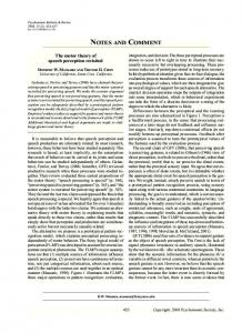
Each individual’s accuracy will, thus, depend on two parameters: (1) the recognition validity, α, defined as the proportion of correct inferences on pairs where only one city is recognized; and (2) the knowledge validity, β, defined as the proportion of correct inferences on pairs where both cities are recognized. If we assume an α of .80 and a β of .70 for all 3 individuals, Figure 1 shows that
Proportion of Correct Inferences
.75
Britta Clemens
.70 .65 Arthur
.60 .55 .50 0
5
10
15
20
Number of Objects Recognized Figure 1. Less-is-more effects illustrated for a recognition validity of α 5 .8 and a knowledge validity of β 5 .7. The performance of Arthur, Britta, and Clemens is indicated by the three points on the curve.
Britta, although she has heard of fewer French cities than Clemens, will achieve the highest number of correct inferences. This example illustrates the less-is-more effect: A person who has heard of fewer objects than another person can still achieve a higher inferential accuracy. Various types of less-is-more effects can be distinguished, depending on whether different levels of knowledge reflect changes within a person over time (e.g., through learning), persons with different levels of expertise in a domain (e.g., laypeople vs. experts), or different domains (although between-domain less-is-more effects can be more difficult to establish; Dougherty et al., 2008). My analysis of the impact of validity dependencies applies to all types of lessis-more effects—that is, wherever inferential accuracy is analyzed as a function of knowledge (irrespective of the source of variation in such knowledge). Analytical investigations into the robustness and scope of the less-is-more effect have yielded several interesting results. For instance, the effect can also occur in tasks that involve comparisons among more than two objects (McCloy, Beaman, & Smith, 2008), as well as in group decision making (Reimer & Katsikopoulos, 2004); Pleskac (2007) and Katsikopoulos (in press) investigated how imperfect recognition memory influences the effect, and Schooler and Hertwig (2005) demonstrated that a less-is-more effect can also arise through forgetting. In addition, Dougherty et al. (2008) showed how the less-is-more effect can arise—in certain environments—through a familiarity-based mechanism. These developments represent important extensions of Goldstein and Gigerenzer’s (2002) model of the recognition heuristic. Although its formal character represents a huge improvement over ill-specified labels (such as availability; see, e.g., Gigerenzer, 1996), crucial processes contributing to recognition-based inference, such as the recognition process, were not formalized in Goldstein and Gigerenzer’s model. A possible consequence of such an omission is discussed in the final part of the present article. Conditions for the Less-Is-More Effect Goldstein and Gigerenzer (2002) showed mathematically that a less-is-more effect will occur if the recognition validity α is larger than the knowledge validity β (although this is not a necessary condition; see Katsikopoulos, in press). In this analysis, it was supposed that α and β remain constant across different levels of recognition knowledge. As they noted, however, “in the real world, the recognition and knowledge validities usually vary when one individual learns to recognize more and more objects from experience” (p. 80). Therefore, Goldstein and Gigerenzer ran a computer simulation that learned the names of German cities according to empirical recognition rates (i.e., the proportion of participants recognizing the city) and recalculated α for each (increasingly larger) set of recognized cities. The recognition validity could thus vary across different levels of recognition knowledge; nevertheless, a less-is-more effect still emerged (see their Figure 3). Although this simulation shows that α does not need to be constant for a less-is-more effect to occur, it is currently unclear how the effect is affected when α (and β) correlate with the number of recognized objects, n (cf. Dougherty
Notes and Comment 591 et al., 2008). Below, I show that a correlation of α or β with n can be critical for the occurrence of the less-is-more effect. Before I turn to this analysis, I give an overview of the empirical support for the less-is-more effect. Empirical Evidence Can the less-is-more effect be observed empirically? As a cautionary note, in many situations, the predicted size of the less-is-more effect is very small, which would lead to statistically significant differences only with extremely large sample sizes. This might be one reason why empirical tests of the effect often rely on simple comparisons of accuracy levels with full versus incomplete knowledge, without running significance tests (there are exceptions; see below). In the studies mentioned in the following overview, no significance test was reported, unless noted. Goldstein and Gigerenzer (2002) reported two demonstrations in support of the less-is-more effect. In the first, they asked a group of American participants to judge which of two cities is larger, both for the 22 largest German cities and for the 22 largest American cities. The participants knew relatively little about German cities; in fact, they had heard of, on average, only about half of the cities. Nevertheless, participants achieved a slightly higher percentage of correct inferences for the German than for the American cities. In Goldstein and Gigerenzer’s (2002) second demonstration, German participants learned to recognize, across a period of 4 weeks, the names of American cities that they had previously not heard of. Despite this increase in recognition knowledge, participants’ inferential accuracy dropped significantly from Week 1 to 4. Using a different domain, Snook and Cullen (2006) asked participants to judge which of two National Hockey League (NHL) players had achieved a larger number of career points. Participants varied greatly in terms of their knowledge about NHL players: Some had heard of more than 100 players, whereas others had heard of only 20. Participants who had heard of many players, however, did not achieve a higher proportion of correct judgments than relatively ignorant participants did. A regression analysis based on the observed data suggested a quadratic relationship between the amount of recognized players and accuracy, with the estimated accuracy decreasing for higher levels of recognition knowledge. Similarly, Frosch, Beaman, and McCloy (2007) found (using a within-participants analysis) that participants scored significantly better in picking, from a set of Britons, the wealthiest one when they did not recognize all individuals in the set, as compared with when they recognized all of them. Other studies have failed to find a (numerical) less-ismore effect, even when α was greater than β. For instance, comparing German participants’ accuracy in judging the sizes of German, Belgian, and Italian cities, Pohl (2006, Experiment 3) reported that participants achieved a significantly higher accuracy in the domains for which they had the most knowledge (German cities) than for the domains about which they were more ignorant (the average knowledge validity for German cities was lower than the average recognition validities for the other domains).
In a forecasting study, Pachur and Biele (2007) asked, for the matches of the 2004 European Soccer Championships, which team the participants thought was more likely to win. Although the average recognition validity was higher than the average knowledge validity,1 accuracy increased monotonically across different levels of recognized teams. The highest accuracy was achieved by those participants who had heard of all or almost all teams. Overall, one may thus argue that the empirical evidence for less-is-more effects in inference tasks is mixed. What if one takes a more comprehensive look that also includes studies that have not explicitly tested the less-is-more effect? Figure 2 plots—for a total of 10 data sets spanning various domains, in all of which the average recognition validity was larger than the average knowledge validity— the accuracy of individual participants as a function of the number of recognized objects (further details about the data sets are given in Table 1).2 Since tests of between-domains less-is-more effects can be ambiguous (Dougherty et al., 2008), and since tests of across-time less-is-more effects are rare (e.g., Goldstein & Gigerenzer, 2002), I focus on less-ismore effects across participants.3 The pattern in each data set is summarized by locally weighted polynomial regression (LOESS) lines (see, e.g., Cleveland & Devlin, 1988). As can be seen, in some data sets, there are indications of a less-is-more effect; in others, there are not. Cues in Natural Environments Validity Dependencies Why is the less-is-more effect sometimes difficult to find empirically? As mentioned above, one possibility is that the effect is often small and can thus easily get masked by noise in empirical data. For instance, for an α of .8 and a β of .7 (assuming they are constant across n), Equation 1 yields a predicted size of the less-is-more effect (defined as the difference between the maximum accuracy and the accuracy with full knowledge) of merely 2.6%. Second, it is possible that people only rarely rely on the recognition heuristic: Hilbig, Erdfelder, and Pohl (2010) showed that a compensatory processing of recognition can diminish or even destroy the less-is-more effect. A third possibility was pointed out by Pachur and Biele (2007), who observed validity dependencies: Participants who recognized more objects also tended to have higher recognition validities and knowledge validities, violating Goldstein and Gigerenzer’s (2002) independence assumption. Because α and β are the main determinants of a person’s overall accuracy (see Equation 1), “a systematic trend toward higher values . . . when more teams are recognized . . . means that with increasing n the overall forecasting accuracy increases as well—the opposite of a less-is-more pattern” (p. 112). How general is Pachur and Biele’s (2007) observation of validity dependencies? Table 1 reports for each of the 10 data sets shown in Figure 2 the corresponding correlation of α with n, r(α, n), and the correlation of β with n, r(β, n). In the majority of the data sets, the correlations are substantial. Interestingly, the values for r(α, n) are sometimes positive and sometimes negative, whereas the values
Proportion of Correct Inferences
Proportion of Correct Inferences
592 Pachur Snook & Cullen (2006, NHL players)
Pohl (2006, Exp. 1, Swiss cities)
Pohl (2006, Exp. 3, Italian cities)
Pohl (2006, Exp. 3, Belgian cities)
Pohl (2006, Exp. 4, islands)
1
1
1
1
1
.8
.8
.8
.8
.8
.6
.6
.6
.6
.6
.4
.4
.4
.4
.4
.2
.2
.2
.2
.2
0
0
100
200
0
Pachur & Biele (2007, soccer)
0
10
20
Hertwig et al. (2008, music artists)
0
0
5
10
0
Hertwig et al. (2008, American cities)
0
5
10
0
Hertwig et al. (2008, companies)
1
1
1
1
.8
.8
.8
.8
.8
.6
.6
.6
.6
.6
.4
.4
.4
.4
.4
.2
.2
.2
.2
.2
0
5
10
15
0
0
50
100
0
0
50
100
0
0
20 40 60 80
5
10
Pachur et al. (2009, American cities)
1
0
0
0
0
10
20
Number of Objects Recognized Figure 2. The relationship between the observed inference accuracy and the number of recognized objects in 10 empirical data sets. Each dot represents 1 participant. The lines represent locally weighted polynomial regression (LOESS) lines. Note that, in all data sets, α . β.
for r(β, n) are mostly positive—an issue discussed further below. In the following, I first examine, via computer simulations, the impact of validity dependencies on the less-is-more effect. Then, I consider possible reasons for the emergence of these dependencies. Validity Dependencies What Is Their Impact on the Less-Is-More Effect? In this section, I systematically examine Pachur and Biele’s (2007) conjecture that validity dependencies—that is, correlations between α and n and between β and n—can
have a major impact on the occurrence of the less-is-more effect (for a related analysis, see Smithson, in press). Is there support for this conjecture? If there is, how large is the relative impact of α’s and β’s correlation with n on the effect? To answer these questions, I ran a computer simulation that sequentially learned the names of 100 objects (yielding 100 levels of n 5 1 . . . 100). The average recognition validity (across all levels of n) was set at .8, and the average knowledge validity was set at .7—a situation for which, assuming validity independence, Goldstein and Gigerenzer (2002) predicted a pronounced less-is-more
Table 1 Relative Changes of the Prevalence and Size of the Less-Is-More Effect Relative Change of LIM Prevalence Size Study Domain α (M ) β (M ) r(α, n) r(β, n) of LIM of LIM Snook & Cullen (2006) Career points of NHL player .84 .80 .14 .23 291.7% 291.8% Pohl (2006, Experiment 1) Population of Swiss cities .86 .75 .02 .17 233.0% 237.3% Pohl (2006, Experiment 3) Population of Italian cities .82 .73 .19 .22 247.2% 248.6% Pohl (2006, Experiment 3) Population of Belgian cities .89 .75 2.13 .06 26.4% 217.4% Pohl (2006, Experiment 4) Size of islands .84 .66 .77 2.04 215.8% 23.8% Pachur & Biele (2007, laypeople) Success of soccer teams .71 .60 .19 .22 236.6% 239.7% Hertwig, Herzog, Schooler, & Reimer (2008) Sales of music artists .61 .57 .32 .16 259.1% 241.5% Hertwig et al. (2008) Population of American cities .83 .68 2.17 .18 214.0% 236.1% Hertwig et al. (2008) Profit of companies .74 .60 2.18 .13 22.2% 227.3% Pachur, Mata, & Schooler (2009, young adults) Population of American cities .91 .76 2.52 .38 260.1% 285.1% Note—LIM, less-is-more effect; NHL, National Hockey League. The relative change of the prevalence of the LIM was calculated as (LIM prevalencedependent 2 LIM prevalenceindependent )/LIM prevalenceindependent 3 100. The relative change of the size of LIM was calculated accordingly.
Notes and Comment 593 effect. The correlation between the recognition validity and the number of recognized objects [r(α, n)] and the correlation between the knowledge validity and the number of recognized objects [r(β, n)] were varied between 21 and 1 in steps of .2. This yielded a total of 11 3 11 5 121 conditions. I manipulated r(α, n) and r(β, n) as follows. First, I created a vector of length 100, representing different values of α, ranging from .60 to 1 (in steps of .004, yielding an average of .8); a vector of length 100, representing different values of β, ranging from .5 to .9 (in steps of .004, yielding an average of .7); and a vector representing the different levels of n, ranging from 1 to 100. Each cell in the “validity vectors” represented the values of α and β, respectively, given the number of recognized objects r(α, n) = .6; r(β, n) = .6
Results Figure 3 shows the average accuracy (across all runs) at different levels of n. For simplicity, results are shown
r(α, n) = .6; r(β, n) = 0
r(α, n) = .6; r(β, n) = �.6
.9
.9
.9
.8
.8
.8
.7
.7
.7
.6
.6
.6
.5
Proportion of Correct Inferences
indicated in the corresponding cell in the “n vector.” In this original form, the two validity vectors were correlated perfectly with the n vector. To create correlations of r(α, n) , 1 and r(β, n) , 1, I reordered a randomly chosen subset of the cells in the validity vectors, with larger subsets for smaller correlations. For instance, reordering 60% of the cells led to an average correlation of around .404. For negative correlations, the validity vectors were flipped. Using the resulting values, I calculated the overall accuracy for each level of n according to Equation 1.4 For each of the 121 conditions, there were 100,000 runs.
0
20
40
60
80
100
.5
0
r(α, n) = 0; r(β, n) = .6
20
40
60
80
100
.5
r(α, n) = 0; r(β, n) = 0 .9
.9
.8
.8
.8
.7
.7
.7
.6
.6
.6
0
20
40
60
80
100
.5
0
r(α, n) = �.6; r(β, n) = .6
20
40
60
80
100
.5
.9
.8
.8
.8
.7
.7
.7
.6
.6
.6
20
40
60
80
100
.5
0
20
40
60
80
40
60
80
100
20
40
60
80
100
r(α, n) = �.6; r(β, n) = �.6
.9
0
0
r(α, n) = �.6; r(β, n) = 0
.9
.5
20
r(α, n) = 0; r(β, n) = �.6
.9
.5
0
100
.5
0
20
40
60
80
100
Number of Objects Recognized Figure 3. Occurrence of the less-is-more effect as a function of the correlation of the recognition validity α and the knowledge validity β with the number of recognized objects n.
594 Pachur only for nine conditions resulting from combining three levels (2.6, 0, and .6) of r(α, n) with the same three levels of r(β, n). The function relating accuracy to n differs greatly among the conditions. In some conditions, there is no less-is-more effect; in others, the effect is amplified as compared with the condition where r(α, n) 5 r(β, n) 5 0 (shown in the center panel in Figure 3). Recall that, in all conditions, α . β. Prevalence of less-is-more effects. To quantify the less-is-more effect, I define it formally as the situation in which there exist two levels of the number of recognized objects, n1 and n2, so that n1 , n2, but f (n1) . f (n2), where f (n) is the accuracy as a function of the number of objects recognized, n (cf. Reimer & Katsikopoulos, 2004). For each condition, I determined the prevalence of less-is-more effects as the proportion of pairs (n1, n2) with n1 n2, for which the less-is-more effect occurs. The left panel in Figure 4 shows the prevalence of lessis-more effects as a function of the size of r(α, n) and r(β, n). The white dot indicates the result under validity independence—that is, when r(α, n) 5 r(β, n) 5 0. There are three main results. First, both r(α, n) and r(β, n), if nonzero, have an influence on the prevalence of less-is-more effects. Second, there is an interaction between r(α, n) and r(β, n). If r(β, n) # 0, a positive correlation between α and n leads to a decrease, and a negative correlation leads to an increase of the prevalence of less-is-more effects. If r(β, n) . 0, however, the opposite pattern holds. That is, a positive correlation between α and n leads to an increase, and a negative correlation leads to a decrease of the prevalence of less-is-more effects. The direction of the influence of r(β, n), by contrast, is independent of the sign of r(α, n): A positive r(β, n) leads to
a decrease, and a negative r(β, n) leads to an increase, of the prevalence of less-is-more effects. The third result is that the influence of r(β, n) is considerably stronger than the influence of r(α, n). As a consequence, even when r(α, n) and r(β, n) have antagonistic effects, the influence of r(β, n) will prevail. For example, the decrease of the prevalence of less-is-more effects when r(β, n) 5 .2 cannot be compensated, even when r(α, n) 5 1. Size of the less-is-more effect. The right panel of Figure 4 shows the results for the size of the less-ismore effect, defined as the difference between maximum accuracy and accuracy with full knowledge (i.e., when n 5 N ). The white dot indicates the result when r(α, n) 5 r(β, n) 5 0. As can be seen, again, both r(α, n) and r(β, n) have an influence on the size of the less-ismore effect, their influences are antagonistic, and the influence of r(β, n) is much stronger than the influence of r(α, n). Moreover, a positive r(β, n) decreases, and a negative r(β, n) increases, the size of the effect. In contrast to the influence on the prevalence of the lessis-more effect, however, the direction of the influence of r(α, n) on the size of the effect does not depend on the sign of r(β, n): A positive r(α, n) increases, and a negative r(α, n) decreases, the size of the effect. As a consequence, when the correlation between n and β is negative, there can be the interesting situation where a positive r(α, n) decreases the prevalence of (as shown above), but increases the size of, the less-is-more effect, or, conversely, where a negative r(α, n) increases the prevalence of, but decreases the size of, the less-is-more effect. Note, however, that this situation may arise rarely in the real world, since negative correlations between n and β are infrequent (see Table 1).
.25
.6
Size of Less-Is-More Effect
Prevalence of Less-Is-More Effect
.7
.5 .4 .3 .2
.15
.10
.05
.1 0
.20
1 .8 .6 .4 –.6 –.8 –1 .2 0 0 –.2 –.4 –.2 –.4 .2 .4 –.6 –.8 –1 1 .8 .6
r (α, n)
r (β, n)
0
–.8 –1 1 .8 .6 .4 .2 –.4 –.6 0 –.2 0 –.2 –.4 .2 .4 .6 –.6 –.8 –1 1 .8
r (α, n)
r (β, n)
Figure 4. The prevalence of the less-is-more effect (left panel) and the size of the less-is-more effect (right panel) as a function of whether and how the recognition validity α and the knowledge validity β are correlated with the number of recognized objects n. The white dots indicate where α and β are uncorrelated with n.
Notes and Comment 595
Proportion of Correct Inferences
Proportion of Correct Inferences
In summary, the computer simulation shows that validity dependencies can influence the prevalence and size of less-is-more effects dramatically. This holds, in particular, for a dependency of β on n. If this dependency is negative, the less-is-more effect is more likely to occur (i.e., it is more prevalent and larger) than when one assumes validity independence (the situation analyzed in Goldstein & Gigerenzer’s, 2002, mathematical analysis); if this dependency is positive, the less-is-more effect is rather unlikely to occur. Since r(β, n) is usually positive (see Table 1) in natural environments, the less-is-more effect will typically be small (or even wiped out). Implications of these results are illustrated in Figure 5, which shows, for the 10 data sets listed in Table 1, the predicted accuracy curves for both the situation where α and β are independent of n (dashed line) and the situation where r(α, n) and r(β, n) take on the empirically observed values reported in Table 1 (solid line).5 The two rightmost columns in Table 1 show the relative changes in the prevalence and size of the less-is-more effect, respectively, under validity dependence and validity independence. For the majority of the data sets, both the prevalence and the size of the less-is-more effect are greatly reduced. For instance, for Snook and Cullen’s (2006) data set, the prevalence rate of less-is-more effects under validity dependence is reduced by more than 90% of the prevalence rate when r(α, n) 5 r(β, n) 5 0 (i.e., a drop from 2.4% to 0.2%). Snook & Cullen (2006, NHL players)
Pohl (2006, Exp. 1, Swiss cities)
What Gives Rise to Validity Dependencies? Validity dependencies have a strong impact on the occurrence of the less-is-more effect. How do these dependencies arise? The correlation between n and β is usually positive (see Table 1), which, in all likelihood, simply reflects that individuals who recognize many objects tend to possess more cue knowledge, know better cues, and/or use the cues more effectively (cf. Dougherty et al., 2008). For the correlation between n and α, however, both positive and negative values are observed (Table 1). Before discussing ways in which correlations between n and α might arise, it is helpful to clarify what a correlation between n and α means. Interestingly, a derivation of the association between α and n based on the known relationship between cue validities and the U value of the Mann–Whitney test (see the Appendix; cf. Martignon & Hoffrage, 2002), yields that 1 + rs . 2 (2) In other words, α should be independent of n. The inconsistency between this and the empirical results suggests that—in contrast to the assumption in the derivation— empirically, the difference between an object’s relative criterion value and its relative probability of being recognized differs systematically across objects. A correlation
α ( n) =
Pohl (2006, Exp. 3, Italian cities)
Pohl (2006, Exp. 3, Belgian cities)
Pohl (2006, Exp. 4, islands)
1
1
1
1
.9
.9
.9
.9
.8
.8
.8
.8
.8
.7
.7
.7
.7
.7
.6
.6
.6
.6
.6
1 .9
.5
Dependent Independent
20 40 60 80 100
.5
Pachur & Biele (2007, soccer)
20 40 60 80 100
.5
Hertwig et al. (2008, companies)
20 40 60 80 100
Hertwig et al. (2008, music artists)
.5
20 40 60 80 100
.5
Hertwig et al. (2008, American cities)
Pachur et al. (2009, American cities)
1
1
1
1
1
.9
.9
.9
.9
.9
.8
.8
.8
.8
.8
.7
.7
.7
.7
.7
.6
.6
.6
.6
.6
.5
20 40 60 80 100
.5
20 40 60 80 100
.5
20 40 60 80 100
.5
20 40 60 80 100
.5 20 40 60 80 100
20 40 60 80 100
Number of Objects Recognized Figure 5. The predicted relationships between inference accuracy and the number of recognized objects for the 10 data sets in Table 1, either assuming that α and β are independent of n (dashed line) or assuming the empirically observed dependencies (solid line; see Table 1).
596 Pachur between α and n thus implies that recognition predicts the criterion value better for larger objects than for smaller objects (yielding a negative correlation) or vice versa (yielding a positive correlation). (A detailed description of this argument can be found in the online supplemental material.) In the following, I discuss how memory and characteristics of the environment could give rise to the asymmetric distribution of recognition validities that a correlation between α and n implies. Memory Computer simulations using the MINERVA memory model (Hintzman, 1988), described in the online supplemental material, show that a negative correlation between n and α can arise as a result of an interaction between memory and the structure of the environment. The rationale is as follows. Recognition results from encountering objects in the environment (e.g., in the media). For instance, the more frequently the name of a tennis player is cited in the newspaper, the more likely a person is to have heard of him. A lower citation frequency, by contrast, produces a lower familiarity signal in memory, leading (in the presence of random error) to less accurate recognition judgments. The distribution of citation frequencies is often skewed, where a large proportion of objects are cited only infrequently in the news and few objects are cited very frequently. In such a skewed distribution, when many objects have been encountered, recognition judgments will less accurately reflect whether there actually was an encounter than when only a few objects have been encountered. Less accurate recognition judgments result in a lower α (Pleskac, 2007), and α thus decreases with increasing n, yielding a negative correlation between α and n. This analysis illustrates the value of specifying a process model of the recognition heuristic that includes a formal account of the recognition process, which Goldstein and Gigerenzer’s (2002) model left unspecified (cf. Dougherty et al., 2008; Dougherty, Gettys, & Ogden, 1999; Marewski & Schooler, 2010). Environment In addition to an interplay between the mind and the environment, aspects of the structure of the environment on their own could also give rise to a correlation between recognition validity and n. Skewed distribution of the criterion variable. Many quantities in the world follow a skewed distribution (e.g., city sizes, wealth, book sales, name frequencies; Clauset, Shalizi, & Newman, 2009), so that there are few very large objects and very many rather small objects. If the target variable in inference is such a quantity, an asymmetric distribution of recognition’s predictive power might arise as follows. In a skewed distribution, the differences between objects in the tail of the distribution are very small, which decreases the chance that recognition correctly reflects the relative criterion value. Therefore, the more objects that are recognized, the lower the ability of recognition to predict the criterion, leading to a decreasing recognition validity. The result is a negative correlation between n and α.
Dynamic environments. In competitive domains (e.g., stock market, sports), the pecking order among the competitors often does not remain stable for long. Because the incentive to rise in rank is higher among higher ranked competitors, changes in rank among the top competitors are more likely than changes among lower ranked competitors. Because recognition responds to changes in criterion ranks rather slowly (but see Schooler & Hertwig, 2005; Serwe & Frings, 2006), it will be a worse predictor for the high-ranked objects than for the entire set of objects, giving rise to a positive correlation between n and α.6 Biases in the mediator. A correlation between n and α can also arise due to specific error patterns in the “mediator” responsible for a connection between recognition and the criterion (Goldstein & Gigerenzer, 2002). In mediating the criterion, the mediator can make two distinct types of errors. First, the mediator can (falsely) give a lot of attention to an object that has a low criterion value, thus committing a “false alarm.” Second, the mediator can (falsely) give little attention to an object, even though it has a high criterion value, thus committing a “miss.” If one of these two types of errors—false alarms or misses—prevails in a particular environment (assuming that, otherwise, the mediator reflects the criterion reliably), a correlation between n and α will arise (i.e., false alarms and misses will give rise to positive and negative correlations, respectively). Summary and Conclusions An overview of various data sets revealed that validity dependencies are common in the real world. Extending the analysis by Goldstein and Gigerenzer (2002), I showed that validity dependencies can have dramatic implications for the prevalence and size of the less-is-more effect. If there is a positive correlation between the number of recognized objects and the knowledge validity—a common constellation in the real world—less-is-more effects are unlikely to occur, even if the recognition validity is higher than the knowledge validity. That is, once the independence assumption is violated, α . β is no longer a sufficient condition for the effect. A positive association of the number of recognized objects with the recognition validity, by contrast, can amplify the less-is-more effect, but this impact is rather weak. Aspects of the environment and memory can give rise to a correlation between the number of recognized objects and the recognition validity. The results offer one explanation why, in the real world, occurrences of the less-is-more effect may be rather rare. More important, they help specify the situations in which the effect is predicted to occur. Author Note I thank Mike Dougherty, Gerd Gigerenzer, Ralph Hertwig, Stefan Herzog, and Tim Pleskac for helpful comments on earlier versions of this article; Dan Goldstein and Rick Thomas for discussions; and Laura Wiles for editing the manuscript. Correspondence concerning this article should be addressed to T. Pachur, Department of Psychology, University of Basel, Missionsstr. 60/64, 4055 Basel, Switzerland (e-mail: thorsten
[email protected]).
Notes and Comment 597 References Clauset, A., Shalizi, C. R., & Newman, M. E. J. (2009). Power-law distributions in empirical data. SIAM Review, 51, 661-703. Cleveland, W. S., & Devlin, S. J. (1988). Locally weighted regression: An approach to regression analysis by local fitting. Journal of the American Statistical Association, 83, 596-610. Cohen, J., Cohen, P., West, S. G., & Aiken, L. S. (2003). Applied multiple regression/correlation analysis for the behavioral sciences (3rd ed.). Mahwah, NJ: Erlbaum. Dougherty, M. R. [P.], Franco-Watkins, A. M., & Thomas, R. (2008). Psychological plausibility of the theory of probabilistic mental models and the fast and frugal heuristics. Psychological Review, 115, 199-211. Dougherty, M. R. P., Gettys, C. F., & Ogden, E. E. (1999). MINERVA-DM: A memory processes model for judgments of likelihood. Psychological Review, 106, 180-209. Frosch, C. A., Beaman, C. P., & McCloy, R. (2007). A little learning is a dangerous thing: An experimental demonstration of ignorancedriven inference. Quarterly Journal of Experimental Psychology, 60, 1329-1336. Gigerenzer, G. (1996). On narrow norms and vague heuristics: A reply to Kahneman and Tversky (1996). Psychological Review, 103, 592596. Gigerenzer, G., Hoffrage, U., & Goldstein, D. G. (2008). Fast and frugal heuristics are plausible models of cognition: Reply to Dougherty, Franco-Watkins, and Thomas (2008). Psychological Review, 115, 230-239. Goldstein, D. G., & Gigerenzer, G. (2002). Models of ecological rationality: The recognition heuristic. Psychological Review, 109, 75-90. Hertwig, R., Herzog, S. M., Schooler, L. J., & Reimer, T. (2008). Fluency heuristic: A model of how the mind exploits a by-product of information retrieval. Journal of Experimental Psychology: Learning, Memory, & Cognition, 34, 1191-1206. Hertwig, R., & Todd, P. M. (2003). More is not always better: The benefits of cognitive limits. In D. Hardman & L. Macchi (Eds.), Thinking: Psychological perspectives on reasoning, judgment and decision making (pp. 213-231). Chichester, U.K.: Wiley. Hilbig, B. E., Erdfelder, E., & Pohl, R. F. (2010). One-reason decision making unveiled: A measurement model of the recognition heuristic. Journal of Experimental Psychology: Learning, Memory, & Cognition, 36, 123-134. Hilbig, B. E., & Pohl, R. F. (2008). Recognizing users of the recognition heuristic. Experimental Psychology, 55, 394-401. Hilbig, B. E., & Pohl, R. F. (2009). Ignorance- versus evidence-based decision making: A decision time analysis of the recognition heuristic. Journal of Experimental Psychology: Learning, Memory, & Cognition, 35, 1296-1305. Hinds, P. J. (1999). The curse of expertise: The effects of expertise and debiasing methods on prediction of novice performance. Journal of Experimental Psychology: Applied, 5, 205-221. Hintzman, D. L. (1988). Judgments of frequency and recognition memory in a multiple-trace memory model. Psychological Review, 95, 528-551. Katsikopoulos, K. V. (in press). The less-is-more effect: Predictions and tests. Judgment & Decision Making. Marewski, J. N., Gaissmaier, W., Schooler, L. J., Goldstein, D. G., & Gigerenzer, G. (2010). From recognition to decisions: Extending and testing recognition-based models for multialternative inference. Psychonomic Bulletin & Review, 17, 287-309. Marewski, J. N., & Schooler, L. J. (2010). Cognitive niches: An ecological model of emergent strategy selection. Manuscript submitted for publication. Martignon, L., & Hoffrage, U. (2002). Fast, frugal, and fit: Simple heuristics for paired comparison. Theory & Decision, 52, 29-71. McCloy, R., Beaman, C. P., & Smith, P. T. (2008). The relative success of recognition-based inference in multichoice decisions. Cognitive Science, 32, 1037-1048.
Pachur, T., & Biele, G. (2007). Forecasting from ignorance: The use and usefulness of recognition in lay predictions of sports events. Acta Psychologica, 125, 99-116. Pachur, T., Bröder, A., & Marewski, J. N. (2008). The recognition heuristic in memory-based inference: Is recognition a noncompensatory cue? Journal of Behavioral Decision Making, 21, 183-210. Pachur, T., & Hertwig, R. (2006). On the psychology of the recognition heuristic: Retrieval primacy as a key determinant of its use. Journal of Experimental Psychology: Learning, Memory, & Cognition, 32, 983-1002. Pachur, T., Mata, R., & Schooler, L. J. (2009). Cognitive aging and the adaptive use of recognition in decision making. Psychology & Aging, 24, 901-915. Pachur, T., Todd, P. M., Gigerenzer, G., Schooler, L. J., & Goldstein, D. G. (in press). When is the recognition heuristic an adaptive tool? In P. M. Todd, G. Gigerenzer, & ABC Research Group, Ecological rationality: Intelligence in the world. New York: Oxford University Press. Pleskac, T. J. (2007). A signal detection analysis of the recognition heuristic. Psychonomic Bulletin & Review, 14, 379-391. Pohl, R. F. (2006). Empirical tests of the recognition heuristic. Journal of Behavioral Decision Making, 19, 251-271. Reimer, T., & Katsikopoulos, K. V. (2004). The use of recognition in group decision-making. Cognitive Science, 28, 1009-1029. Schooler, L. J., & Hertwig, R. (2005). How forgetting aids heuristic inference. Psychological Review, 112, 610-628. Serwe, S., & Frings, C. (2006). Who will win Wimbledon? The recognition heuristic in predicting sports events. Journal of Behavioral Decision Making, 19, 321-332. Smithson, M. (in press). When less is more in the recognition heuristic. Judgment & Decision Making. Snook, B., & Cullen, R. M. (2006). Recognizing National Hockey League greatness with an ignorance-based heuristic. Canadian Journal of Experimental Psychology, 60, 33-43. Notes 1. The average validities are calculated by first determining the validities for each individual participant (as defined above) and then averaging the individual parameters across participants. 2. I thank Stefan Herzog, Rüdiger Pohl, and Brent Snook for providing their raw data. 3. These studies thus fulfill the criteria for a proper test of the lessis-more effect, as stipulated by Dougherty et al. (2008), involving a comparison of individuals “with different levels of knowledge all raised in the same ecology making inferences about objects within the same reference class” (p. 206). 4. That is, the simulation assumed implicitly that people apply the recognition heuristic in every case they can. Although this assumption is not supported empirically (people usually pick the recognized objects in only 80%–90% of the cases), for comparability with Goldstein and Gigerenzer’s (2002) analysis, I nevertheless retained this assumption. Further analyses showed that more realistic adherence levels led to qualitatively very similar results. 5. For the uncorrelated case, these predictions were based on putting the observed α and β into Equation 1. For the correlated case, the predictions were generated using simulations similar to those reported above. 6. This possibility holds irrespective of the shape of the criterion distribution, which, as discussed above, can also produce a correlation between α and n. SUPPLEMENTAL MATERIALS An extended discussion and analysis of the correlations in this article may be downloaded from http://pbr.psychonomic-journals.org/content/ supplemental.
(Continued on next page)
598 Pachur Appendix Recognition Validity As a Function of the Number of Recognized Objects Each item from a set of objects has a recognition rank and a criterion rank. The recognition rank orders the objects according to the number of individuals recognizing them. The criterion rank orders the objects according to their criterion value. Using the connection between cue validity and the U value for the Mann–Whitney test (cf. Martignon & Hoffrage, 2002), we can express the recognition validity α, given n recognized objects, as
α ( n) =
n( n + 1) − S ( n) 2 , n( N − n)
n( N − n) +
(A1) where S(n) is the sum of criterion ranks Rcrit of the n recognized objects. What is the expected value of S(n)? As a first step, what is the expected criterion rank of the nth recognized object, given that n objects are recognized: Rcrit (n)? Put differently, what is the expected criterion rank of the object with a particular recognition rank? Assume that objects are learned in the order of their recognition ranks, Rrec , so that n 5 Rrec (cf. Goldstein & Gigerenzer, 2002); that the expected rank depends only on the recognition rank—that is, Rcrit (n) 5 f (Rrec ); and that the function relating Rcrit and Rrec is linear. Think of the criterion ranks and the recognition ranks as two variables that have the same variance (assuming there are no ties) and are correlated by rs (i.e., the recognition correlation; Goldstein & Gigerenzer, 2002). Generally, a variable Y is predicted linearly by another variable X as Y 5 B0 1 BYX 3 X, where the intercept B0 5 MY 1 MX 3 BYX and the slope BYX 5 rXY 3 sY /sX (see Cohen, Cohen, West, & Aiken, 2003, p. 33). Applied to the present case, Rcrit (n) 5 M(Rcrit ) 1 M(Rrec ) 3 BRcritRrec 1 BRcritRrec 3 Rrec . Because Rrec and Rcrit both range from 1 to N, both the average recognition rank, M(Rrec), and the average criterion rank, M(Rcrit ), equal (N 1 1)/2. Additionally, because Rrec and Rcrit both represent ranks, they have the same variance (sRcrit /sRrec 5 1) and, therefore, BRrec Rcrit 5 rs . Consequently, we obtain as our first result the expected criterion rank of the nth recognized object expressed as a linear function of the object’s recognition rank:
(
) (
)
Rcrit ( n) = N + 1 − N + 1 × rs + rs × Rrec . (A2) 2 2 As a second step, what is the sum of the expected criterion ranks across all n recognized objects? For that purpose, we need to multiply the intercept (the left-hand side of Equation A2) by n and replace Rrec with the sum of the recognition ranks of the n recognized objects, which is n( n + 1) n ∑ i =1 R reci = 2 . The sum of the expected criterion ranks across all n recognized objects is thus
(
) (
)
n( n + 1) S ( n) = n N + 1 − N + 1 × rs + rs × . 2 2 2 By putting Equation A3 into Equation A1, we obtain
α ( n) =
This can be simplified to
n( N − n) +
(
)(
)
n( n + 1) n( n + 1) − n N + 1 − N + 1 × rs − rs × 2 2 2 2 . n( N − n)
α ( n) = 1 −
1 − rs 1 + rs = . 2 2
(Manuscript received October 18, 2009; revision accepted for publication March 3, 2010.)
(A3)
(A4)