Psychonomic Bulletin & Review 2009, 16 (3), 583-593 doi:10.3758/PBR.16.3.583
Notes and Comment Purely relative models cannot provide a general account of absolute identification Scott D. Brown
University of Newcastle, Callaghan, New South Wales, Australia
A. A. J. Marley
University of Victoria, Victoria, British Columbia, Canada and
Pennie Dodds and Andrew Heathcote
University of Newcastle, Callaghan, New South Wales, Australia Unidimensional absolute identification—identifying a presented stimulus from an ordered set—is a common component of everyday tasks. Laboratory investigations have mostly used equally spaced stimuli, and the theoretical debate has focused on the merits of purely relative versus purely absolute models. Absolute models incorporate substantial knowledge of the complete set of stimuli, whereas relative models allow only partial knowledge and assume that each stimulus is compared with recently observed stimuli. We test and refute a general prediction made by relative models, that accuracy is very low for some stimulus sequences when the stimuli are unequally spaced. We conclude that, although relative judgment processes may occur in absolute identification, a model must incorporate long-term referents to explain performance with unequally spaced stimuli. This implies that purely relative models cannot provide a general account of absolute identification.
Absolute identification requires participants to identify which stimulus has been presented from a prespecified set. In general, people are unable to accurately identify more than about 8–10 stimuli that vary on a single psychological dimension, which is surprising when comparative judgments with the same stimuli (i.e., judging whether one stimulus is less than, equal to, or greater than another stimulus) are completely accurate. For over 20 years, theories of absolute identification have been divided along a continuum from purely absolute accounts to purely relative accounts (for reviews, see Brown, Marley, Donkin, & Heathcote, 2008; Stewart, Brown, & Chater, 2005). Absolute models assume some form of memory for the magnitude of each stimulus in the set—a set of long-term referents that represent the stimuli. Relative models make a more parsimonious assumption by representing the stimuli with a limited set of partial information. Usually, relative models assume that the only long-term memory is for a single scale factor related to the spacing of the
s timuli—that is, to the magnitude differences between adjacent stimuli. The relative approach has proven successful in magnitude estimation tasks (e.g., Luce & Green, 1974; Marley, 1976), and the superficial similarity between the tasks suggests that the same approach may work in absolute identification. The theoretical debate has progressed mainly by pairwise comparison of particular absolute and relative models—for example, Marley and Cook (1984) versus Laming (1984); Petrov and Anderson (2005) versus Stewart et al. (2005); and Stewart et al. (2005) versus Brown et al. (2008). There have been one or two attempts at a more general comparison, but these have proven less diagnostic than was hoped (see, e.g., Brown, Marley, & Lacouture, 2007; Stewart, 2007; Stewart et al., 2005, Experiment 2). Here, we present a classwise comparison based on key differences in the way absolute and relative models map from the stimulus to the response space. Rather than relying on small differences in quantitative goodness of fit, we identify a qualitative failure of relative models, caused by their core structure. In particular, we show that relative models make very strong and surprising predictions for experiments in which unequally spaced stimuli are used. We then test these predictions with a new experiment that addresses a potential limitation of past research. We focus on absolute identification experiments with unequally spaced stimuli presented with feedback, which means that participants are informed of the correct response after each trial. Feedback is almost always presented in numeric format (e.g., as a digit on a computer screen), and so researchers have used the term numeric feedback (Holland & Lockhead, 1968, p. 412). The numeric nature of feedback is important in our discussion of relative models, especially of the relative judgment model (RJM; Stewart et al., 2005). In fact, we show that relative models—including the RJM—are unable to account for certain aspects of data from experiments with unequally spaced stimuli. Although it is not the model described by Stewart et al., an extended version of the RJM can account very accurately for unequally spaced designs.1 However, the extension contradicts the core assumptions of the relative account of absolute identification, transforming the relative judgment model into an absolute judgment model, or at least into a hybrid absolute–relative judgment model. Absolute Versus Relative Stimulus Representations Absolute and relative models of absolute identification assume fundamentally different psychological representations. All absolute models include a flexible long-term
S. D. Brown,
[email protected]
583
© 2009 The Psychonomic Society, Inc.
584 Brown, Marley, Dodds, and Heathcote memory representation of the entire set of stimuli used in an experiment. For example, Marley and Cook (1984) assumed end anchors and an attention mechanism that together yield a long-term representation of the stimulus context and, indirectly, of stimulus magnitude. Petrov and Anderson (2005) posited explicit anchors that provide referents for the magnitude of each stimulus. In theories based on Lacouture and Marley’s (1995) bow mapping (including Brown et al., 2008; Lacouture & Marley, 2004), both end anchors and a referent for each stimulus have been used. By contrast, a fundamental property of relative models is that they explicitly deny the use of memories for stimulus magnitudes. Instead, they use only magnitude differences between stimuli presented on successive trials and assume that equal stimulus differences are mapped to equal differences on a response scale. Relative models have enjoyed considerable success and have been able to account for almost all of the data accounted for by the more complex absolute theories (see Stewart, 2007; Stewart et al., 2005). However, our analyses suggest that this success is a product of the way in which researchers have traditionally designed their experiments, almost always using designs in which the stimuli are equally spaced and the feedback respects this equal spacing. This matches the assumption underlying relative accounts but runs the risk that they will not generalize to absolute identification in the real world, where stimuli are often not equally spaced. There have been isolated investigations into the effects of unequally spaced stimuli (Lacouture, 1997; Lockhead & Hinson, 1986). However, in these experiments, a withinsubjects design has always been used to compare equal and unequal spacing conditions. This may have prompted participants to take particular note of the stimulus structure and encouraged them to use an absolute, rather than a relative, processing mode—whether or not that mode was their default. Our experiments address this possibility by manipulating unequal spacing conditions between subjects. The representations used by relative accounts of absolute identification make a powerful and surprising prediction: that unequally spaced stimuli should result in very poor accuracy for certain trial sequences. On the other hand, absolute accounts predict that data from experiments with unequally spaced stimuli should not be radically different from standard data. To illustrate the point, consider the relative judgment models of Laming (1984), Holland and Lockhead (1968), and Stewart et al. (2005) and, for simplicity of the example, ignore sequential effects. These models depend critically on a single estimate for the difference between adjacent stimulus magnitudes. This spacing estimate is used to scale the psychological difference between the current stimulus and the previous stimulus into a difference in response units. The resulting estimate of the response difference between the current and previous stimuli is then added to the numeric feedback for the previous trial.2 This numeric feedback informs the participant of the correct response for the previous stimulus, and so, when the estimated response difference between the previous and current stimuli is added, a response can be generated for the current stimulus.
When the stimuli used in an experiment are unequally spaced, this process breaks down in the obvious manner. The single estimate used for the spacing between adjacent stimuli cannot capture all of the different spacings that exist between different stimuli. The relative model is forced into a compromise when scaling from stimulus differences to response differences, using some average estimate of the spacing between stimuli. This average estimate leads to errors whenever the current and prior stimuli are separated by spacings that are different from the average estimate. We will develop the argument above more formally in the Appendix. There, we will set out a very basic model that captures the core elements of relative judgment but includes no extra components, such as random variability or sequential effects. We will show that when stimuli are unequally spaced, the basic model predicts very low accuracy for certain combinations of current and prior stimulus magnitudes, regardless of the values given to the model’s parameters. Below, we will test this prediction using data from an experiment with unequally spaced stimuli, replicating Lockhead and Hinson’s (1986) design. The simple model we will analyze in the Appendix does not include many of the extra components used in cutting-edge relative models, so our analyses will not apply perfectly to those accounts. Therefore, we also will show that the leading relative model (the RJM) cannot account for our data or those from one of Lacouture’s (1997) unequal spacing experiments. These analyses will confirm that the problems observed in cutting-edge relative models are the same as those found in the basic architecture analyzed in the Appendix. Method Participants Introductory psychology students from the University of Newcastle took part in the experiment, receiving course credit as compensation: 10 participants in the low-spread condition and 8 in each of the other two conditions.
Low Spread
Even Spread
High Spread
73
76
79
82
85
88
91
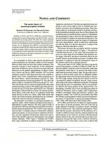
Intensity (dB) Figure 1. Schematic illustration of the stimuli used in the three different conditions.
Notes and Comment 585 Stimuli There were three spacing conditions: low spread, even spread, and high spread. In each condition, the stimuli were three 1000-Hz tones of different intensities. The range of tone intensities was different in each condition, as illustrated in Figure 1. In the even-spread condition, the tones were equally spaced at 79, 82, and 85 dB. The stimuli in the other conditions were identical, except that in the low-spread condition, Stimulus 1 was made less intense (73 dB), and in the highspread condition, Stimulus 3 was made more intense (91 dB). Procedure Each participant was randomly assigned to the low-, even-, or high-spread condition. Each condition had three phases: digit identification, practice, and a test phase. The digit identification block was 90 trials in length, during which the participants responded to a series of electronically prerecorded numbers (1, 2, or 3). They were asked to press the corresponding number key on a regular keyboard; each number was played via headphones 30 times, in random order. This phase was intended to examine baseline response times for unambiguous stimuli, so that differences in mean response times for the three different response buttons (and fingers) could be identified. During practice, each of the three tones was played once, in ascending order of intensity. Each tone was labeled with the number 1, 2, or 3, which appeared on screen while the tone was played. The participants were required to press the corresponding key to continue—for example, “This is tone number 1, if you think you have heard this tone, press 1 to continue.” The test phase had 10 blocks. In each block, each stimulus was presented 30 times, with the order of the 90 trials being randomized. On each trial, a visual cue (1) was displayed for 500 msec; then the stimulus was played for 1,000 msec, and the participant had up to 20 sec to respond. If no response was made, the next trial was presented, and a missing value was recorded. If a response was incorrect, the correct answer was displayed on the screen for 1,000 msec. If the response was correct, “Correct” was displayed on the screen for 1,000 msec. The participants were required to take a minimum 30-sec break between the blocks.
Results Response times shorter than 180 msec or longer than 5 sec were removed from the analysis, which accounted for fewer than 1% of the trials in each condition. The results from the digit identification block showed that there were no substantial differences in response time across Stimuli 1–3; on average, response times were 642, 678, and 635 msec, respectively, and this pattern was maintained within the three experimental conditions. Figure 2 illustrates the absolute identification results. Results in the even-spread condition were typical of traditional absolute identification tasks. Mean response time (top row, middle panel) was longer for the middle stimulus than for the edge stimuli, although the mean difference was slight (59 msec). Response probabilities (bottom row, middle panel) show that the correct response was most frequent for each of Stimuli 1–3: 78%, 79%, and 87%, respectively. There was a slight asymmetry, with the softest stimulus identified less accurately, and more slowly, than might be expected, relative to the loudest stimulus. The results shown in Figure 2 replicated the key aspects of Lockhead and Hinson (1986). Responses to the privileged stimuli (the ones with greater separation) were more accurate in the low- and high-spread conditions than in the even-spread condition [t(16) 5 3.7, p 5 .001, and t(14) 5 4.4, p 5 .001, respectively]. Mean response times for the privileged stimuli were also shorter, although the differences were not significant [t(16) 5 0.9, p . .05, and t(14) 5 1.4, p . .05, respectively]. These advantages are unsurprising, since in each case, the stimulus itself was different, either much louder or much softer.
Spread
Mean RT (sec)
Low
Even
High
1.0 0.9 0.8 0.7
Response Probability
1.0
Response 1
.8
2 3
.6
SAMBA
.4 .2 0 1
2
3
1
2
3
1
2
3
Stimulus Figure 2. Mean response times (RTs; top row) and response probabilities (bottom row) for the low-spread, evenspread, and high-spread conditions. The triangle, circle, and inverted triangle symbols depict data associated with Responses 1, 2, and 3, respectively. Error bars are 61 standard error, calculated across participants, assuming normal distributions of means in the population. The dashed lines join predictions from the SAMBA model.
586 Brown, Marley, Dodds, and Heathcote What is more interesting is that the remaining two stimuli were confused more often in the low- and high-spread conditions than in the even-spread condition, even though these two stimuli were physically identical across pairs of conditions. For example, Stimuli 1 and 2 were physically identical in the even-spread and high-spread conditions (79 and 82 dB in both cases), yet they were confused more often in the high-spread condition than in the even-spread condition. In the even-spread condition, Response 1 was given on 11% of the presentations of Stimulus 2, but this rose to 19% in the high-spread condition, and the difference was significant [t(14) 5 2.6, p 5 .014]. Similar patterns occurred (with smaller magnitudes) for the other identical stimulus/response pairs. An Absolute Account of the Data Theories in which absolute processes are used naturally account for data from unequally spaced stimuli, because they include complete knowledge of the stimulus set, including long-term memories for the magnitudes of all the stimuli in the set. When the spacing of the stimuli changes, so do these referents. The tracking process that carries out these changes may be specified in great detail (e.g., Petrov & Anderson, 2005; Treisman & Williams, 1984) or not (e.g., Brown et al., 2008), but nevertheless, all absolute models include the necessary components. To illustrate, we will use Brown et al.’s (2008) model (SAMBA). SAMBA assumes that the magnitude of a stimulus is estimated in a noisy and error-prone fashion, which is then compared against long-term memories (referents) for each stimulus. When the physical spacing of certain stimuli is small, relative to the average spacing of stimuli in the entire set, so too is the difference between their referents. Since decisions are based on comparison with these referents, greater confusion is predicted between stimuli that are closer together, relative to the overall context of the experiment—just as was observed in the data. In Figure 2, the dashed lines join predictions from SAMBA, for both response times (top row) and response probabilities (bottom row). SAMBA’s account of the data is very parsimonious; exactly the same parameter values are used to generate predictions for all three experimental conditions. The different predictions arise without parameter changes because the different stimuli in the three conditions provide different long-term referent values. These referents capture the critical qualitative patterns in both response times and response probabilities. The quantitative fit to the data is quite good, with all predicted response probabilities falling within .05 of the corresponding observed probabilities (root-mean squared error [RMSE] 5 .026). SAMBA’s predictions were generated by adjusting the parameters used by Brown et al. (2008) to fit data from the equally spaced condition in Lacouture’s (1997) experiment. To fit the present data set, four parameters were changed. One parameter was adjusted to fit the overall level of accuracy (η 5 16); larger values of η endow the model with improved memory for the context of the experiment, allowing more precise estimates of stimulus magnitudes. A second parameter was adjusted to fit the overall level of response times (C 5 447); larger values of C correspond to more
caution in evaluating evidence for the different responses. Finally, two anchor values (L and U ) were changed to accommodate the asymmetry in the data; these anchor values describe the range of stimuli that the observer set as relevant for this experiment. Response accuracy is maximized if the range is set identical to the range used in each particular stimulus condition, but observers typically do not quite manage this. We fixed L to be 6 dB quieter than the quietest tone in each condition, and U to be 3.3 dB louder than the loudest in each condition. An even better fit to the data—particularly the response time asymmetry—could have been obtained by allowing differences in the anchors between conditions. Such differences are plausible, given the between-subjects manipulation, but our arguments do not rely on small differences in quantitative fit, and so the extra complexity is not necessary. SAMBA estimates stimulus magnitudes by using a selective attention mechanism based on Marley and Cook’s (1984) rehearsal model. The details are in Brown et al. (2008), but the important point is that the averages of these magnitude estimates serve as referents. Magnitude estimates are expressed as ratios in the interval [0, 1], with 0 representing the lower anchor (L) and 1 representing the upper anchor (U ). With the parameters above, in the evenspread condition, the average magnitude estimates for the three stimuli are {.4, .59, .78}, and these estimates capture the even spacing of the physical stimuli. In the low-spread and high-spread conditions, the average magnitude estimates are {.29, .71, .85} and {.29, .43, .85}, respectively. The latter two sets of estimates capture the relevant threeto-one stimulus spacings without the need for changes in parameters between conditions. The Relative Account Relative models make the strong prediction that response accuracy for certain stimulus sequences will be very low when stimuli are unequally spaced. For example, consider the relative models proposed by Laming (1984) and Stewart et al. (2005). Both models depend critically on a memory for the average spacing between adjacent stimulus magnitudes (λ in Stewart et al.’s model, β in Laming’s). Throughout this article, we will use the symbol Zi to represent the physical magnitude of the stimulus presented on trial i, measured on a logarithmic scale. The symbol Si will be used for the rank of that stimulus within the entire set of stimuli experienced by a participant. In the evenspread condition of our experiment, we used three stimuli with physical magnitudes of 79, 82, and 85 dB. Relative accounts of absolute identification operate using the knowledge that 3 dB separates adjacent stimuli, as follows. Suppose that the stimulus presented on the previous trial was Zn21 5 79 dB (Sn21 5 1) and the stimulus presented on the current trial is Zn 5 82 dB (Sn 5 2). The core elements of a relative model would operate by (1) estimating the magnitude difference between the current and previous stimuli (in this case, 82 2 79 dB 5 13-dB difference); (2) transforming the difference estimate into the numerical response scale, using the knowledge that adjacent stimuli are separated by 3 dB, so that the 13-dB difference is transformed to a difference of 11 response; and (3) con-
Notes and Comment 587 Spread Low
Even
High
Response Probability
1.0 .8 Response .6
1 2
.4
3 RJM
.2 0 1
2
3
1
2
3
1
2
3
Stimulus Figure 3. Data (points) and predictions (dashed lines connecting predicted values) from the RJM.
verting the response difference into a response by adding it to the correct response from the previous trial, which is known by feedback. Thus, the response on the current trial would be the 11 difference added to the previous correct response (1), yielding Response 2 (which is correct). When the stimuli are unequally spaced, this process breaks down. In our high-spread condition, three stimuli were used with intensities of 79, 82, and 91 dB; the loudest stimulus was much louder than before, but the other two were unchanged. The participants performed quite well in this condition, with better than 84% accuracy for each of the three stimuli. However, consider the relative judgment account of the same trial sequence as above; when stimulus Zn21 5 79 dB (Sn21 5 1) is followed by stimulus Zn 5 82 dB (Sn 5 2), the magnitude difference is the same as before, 13 dB. However, if the observer’s long-term memory is based on the average difference between adjacent stimuli, they will use λ 5 6 dB. This causes the observed magnitude difference to be transformed into a numerical response difference of only 1½. When this response differences is added to the numeric feedback from the previous trial (1), the model predicts that the response given for the current trial should be equally likely to be 1 (incorrect) as 2 (correct). Manipulating λ can solve this particular problem—for example, by using λ 5 3 dB. However, this simply shifts the problem to other stimulus sequences (e.g., then all trials on which Stimulus 2 follows Stimulus 3 will be classified incorrectly). This type of reasoning is formalized in the Appendix. Figures 3 and 4 illustrate that this exact problem arises even in the fit of a much more complicated relative model, the RJM of Stewart et al. (2005). In this section, we will focus on the RJM as described by Stewart et al.’s text and equations. A personal communication (June 11, 2008) has revealed that Stewart et al. actually implemented a different version of their model, at least when dealing with experiments using unequally spaced stimuli. We will call that model the extended RJM and will consider it carefully in the next section. Figure 3 shows that the global fit of
the RJM is quite good, with RMSE 5 .042, which is in the same ballpark as SAMBA’s fit (RMSE 5 .026). When fitting the RJM, we adjusted four parameters: one for the scaling of stimulus differences to response differences (λ), one for the effect of the prior trial on the current decision (α1), a variance parameter (σ), and a decision threshold (χ1). We had to allow the RJM to have different parameter values for the equally spaced (λ 5 0.786 dB, α1 5 .312, σ 5 .208, χ1 5 0.702, and χ2 5 4 2 χ1) and unequally spaced (λ 5 2.016 dB, α1 5 .087, σ 5 .092, χ1 5 1.36, and χ2 5 4 2 χ1) conditions. The different values of the spacing parameter, λ, reflect the very different stimulus spacing conditions in the equal versus the unequal spacing conditions.3 These extra parameters (eight, as opposed to the four used by SAMBA) provide the RJM with some extra flexibility, which may concern some readers; however, we were unable to find a common set of parameters that gave a reasonable fit to all three conditions. We also explored even greater parameter freedom for the RJM, by allowing independent parameters for the two response thresholds (χ1 and χ2); this version of the model performed only marginally better than the symmetric version described above. Note that the RJM does not make predictions for response times, so Figure 3 shows only response probabilities. The previous discussion suggests that relative accounts predict very low accuracy for particular stimulus transitions, such as those between Stimuli 1 and 2 in the highspread condition and Stimuli 2 and 3 in the low-spread condition. Figure 4 graphs the accuracy associated with each stimulus (shown using different symbols), conditional on the previous stimulus (given by the x-axes). The three columns of Figure 4 show these graphs separately for the low-spread, even-spread, and high-spread conditions. The top row shows just the data, the second row shows corresponding predictions from SAMBA, and the bottom row shows the predictions made by the RJM. The top row of Figure 4 shows that the participants performed quite well on all stimulus transition sequences; even the very worst accuracy was still 71% (when Stimu-
588 Brown, Marley, Dodds, and Heathcote Spread Low
Even
High
1.0 .8
Data
.6 .4
Response Accuracy
1.0 .8
SAMBA
.6 .4 1.0 .8
RJM
.6 .4
Stimulus 1
2
3
1
2
3
Previous Stimulus
1
2
3
1 2 3
Figure 4. Response accuracy for each stimulus conditioned on the previous stimulus (x-axis): Data (top row) and predictions from the SAMBA model (middle row) and the RJM (bottom row). The three columns correspond to the low-spread, even-spread, and high-spread conditions.
lus 1 followed Stimulus 3 in the even-spread condition). SAMBA’s predictions, shown in the second row, match the data quite well (RMSE 5 .059), and the greatest mismatch between the data and SAMBA’s predictions is only .12. In contrast, the predictions for the RJM, on the third row, are very different from the data. Just as was expected, the predicted accuracy for some stimulus transitions is around 50%. The overall RMSE for RJM’s fit to the sequential data is more than three times that of SAMBA (.19), as is the greatest mismatch between the sequential data and predictions (.41). These analyses demonstrate that the apparently adequate account of the data provided by the RJM in Figure 3 was really a consequence of averaging together large overpredictions for some conditional accuracy values, together with large underpredictions for others. We tried to remedy this misfit by adjusting the free parameters of the RJM solely to optimize the fit shown in Figure 4, ignoring the overall mean response probabilities shown in Figure 3. This analysis resulted in a slight improvement in fit, but not enough to change the conclu-
sions to be drawn, nor did it change the predictions of extremely poor performance for certain stimulus transitions. When the model was endowed with almost double the number of free parameters (an extra two for asymmetric response criteria, plus independent free parameters for all three conditions) and when all of those parameters were adjusted to optimize fit for Figure 4, the overall RMSE for the RJM was still double that of SAMBA (at .12) and the worst misfit was still very large (.31). Lacouture (1997) Lacouture (1997) also studied absolute identification with unequally spaced stimuli. He used a larger stimulus set, which has the consequence that relative models are less able to trade off underprediction and overprediction of the conditional data in order to provide an apparently adequate fit to the unconditional data. In one of his simplest conditions, he used a standard design with 10 lines of increasing length that were equally log-spaced, except for a large gap between the central pair of lines that was six
Notes and Comment 589 1.0
Accuracy
.8 .6 .4 .2
Data RJM
0 1
2
3
4
5
6
7
8
9
10
Response Figure 5. Response accuracy for Lacouture’s (1997) large central gap condition (points) and predictions from the RJM (dashed lines). Error bars show 61 standard error, assuming binomial distributions.
times as large as the other gaps; using arbitrary units4 for log-length, the lines’ lengths were {1, 2, 3, 4, 5, 11, 12, 13, 14, 15}. The data from this condition were very similar to those observed under standard conditions, except for improved response accuracy and latency for stimuli adjacent to the large gap. Figure 5 illustrates these data, following Lacouture’s analysis: plotting accuracy conditioned on the response, rather than the customary conditioning on the stimulus. Similar effects can be observed with either analysis, but they are somewhat clearer in the responseconditioned version. Donkin, Brown, Heathcote, and Marley (2009) demonstrate that SAMBA fits these data well (RMSE 5 .08), while simultaneously accounting for the associated response times and for both types of data for Lacouture’s (1997) other stimulus-spacing conditions, all using the same set of parameters. Our analyses (see the Appendix) show that the core architecture that underlies relative models makes inappropriate predictions for the choice data. To confirm that these problems are not limited to the basic relative architecture, we also fit the RJM to Lacouture’s data. We optimized the RJM’s parameters to fit only the data shown in Figure 5 (σ 5 0.074, λ 5 1.75, and C 5 .136; we could not obtain a better fit by adjusting the five sequential effect parameters α1–5). Other parameter settings allow the RJM to capture the accuracy values for Responses 2–4 and 7–9 somewhat better, but always at the expense of far worse predictions for other responses. As would be expected from our analytic results, the RJM fits the data very poorly (RMSE 5 .18). The relative account of Lacouture’s (1997) data fails in exactly the manner predicted by our analysis in the Appendix. There is a tension in the model between transforming the small spacing between Stimuli 1–5 and 6–10 (just one stimulus spacing unit) to numerical differences on the response scale, and transforming the large gap between Stimuli 5 and 6 (six stimulus spacing units) to a numerical difference on that scale. The RJM settles on a compromise solution, estimating the spacing parameter at λ 5 1.75 spacing units. Of course, this compromise fails for certain stimulus transitions. For example, it makes inappropriate predictions whenever the current and previous
stimuli lie on opposite sides of the large gap (i.e., when the current stimulus is between 1 and 5 and the prior stimulus was between 6 and 10, or vice versa). These predictions are confirmed by the predicted response probabilities from the RJM fits; for example, when the stimulus given on the previous trial was the largest one (10) and the current stimulus was the smallest (1), the RJM always predicted an incorrect response (3). Lacouture’s (1997) participants did not show such behavior. Stimulus 10 was followed by Stimulus 1 a total of 21 times, but not once did this elicit Response 3. Instead, 17 responses were correct (1), and the other 4 were all just 1 response away (2). Similar patterns were observed for many other stimulus sequence pairs that involve either very large or very small jumps between successive stimuli, and these have resulted in near-chance prediction of the conditional accuracy values by the RJM (RMSE 5 .44). In contrast, SAMBA fits these same values with RMSE 5 .17 (Donkin et al., 2009), with the misfit due mostly to a failure to capture the asymmetry in the data due to the responses to Stimuli 4 and 5 being less accurate than those to Stimuli 6 and 7. Rescuing the Relative Account The analyses above suggest that purely relative accounts of absolute identification must fail when stimuli are unequally spaced. In this section, we will present two ways by which the relative account can better address data from unequally spaced stimuli. However, a side effect of both approaches is an increase the amount of long-term stimulus magnitude information used by the model. In each case, this changes the theoretical account from a purely relative one to either a purely absolute one or a hybrid account that falls somewhere in between the two poles. Mapping the Numeric Feedback to Stimulus Magnitude In our analysis of the RJM above, Zn and Zn21 are the physical magnitudes of the current and previous stimuli, measured on a log scale. The difference between these magnitudes is scaled to a difference on the response scale by the parameter λ. Finally, this response scale difference is
590 Brown, Marley, Dodds, and Heathcote added to the feedback given to the participant on the previous trial. This feedback is invariably numeric (one of the digits 1, 2, . . . , N ). For example, in the low-spread condition of our experiment, the physical stimulus magnitudes were 73, 82, and 85 dB. When Stimulus 3 was given, the feedback provided to the participants after their response was the label 3, not the physical magnitude of the stimulus (85 dB). Stewart et al. (2005) extended the RJM to accommodate unequally spaced data from Lockhead and Hinson’s (1986) experiment by assuming that the feedback provided to the model about the correct answer for the previous trial (i.e., the label 1, 2, or 3) is transformed by the observer back into a physical stimulus magnitude (e.g., they assume that the observer transforms the label 3 back to the magnitude 85 dB, or some representation of that). There are two problems with this extended RJM. The first problem is that the extension was never mentioned in print. The reader would naturally assume the conventional definition of feedback: the numeral associated with the correct response. Stewart et al. (2005) reinforced this assumption in three ways. First, they cited Holland and Lockhead’s (1968) model, which explicitly uses numeric feedback, as a basis for their own. Second, Stewart et al. carefully defined a symbol for feedback that was different from the one used for stimulus magnitude. Third, and most explicit of all, the text above Stewart et al.’s Equation 8 clearly used numeric feedback. There, stimulus ranks (Sn21) were used for feedback, whereas psychological magnitudes [written as Aln(r)Sn21, which is equal to Zn21] were used for stimulus differences. This clearly shows that the model Stewart et al. described is the one we have implemented, not the extended RJM. It is surprising that the unusual definition of feedback required for the extended RJM was not discussed by Stewart et al. This omission is particularly surprising because the extended RJM makes a very powerful assumption about the psychological processes in question—that the observer can somehow transform numeric feedback about the stimulus into information about absolute stimulus magnitude. The second, and more serious, problem with Stewart et al.’s (2005) assumption is that it violates the very heart of their work. On page 892, Stewart et al. write:5 “What is admitted to the decision process on trial n is not some representation of the magnitude of Sn but a representation of the difference between Sn and Sn21.” Allowing the assumption that the feedback label (Fn21) can be transformed by the observer into the stimulus magnitude (Zn21) perfectly solves the problem of fitting the data for unequally spaced stimulus sets. However, making this assumption directly contradicts the core of their model—that stimulus magnitudes are not admitted to the decision process. On a deeper level, assuming that the observer can transform numerical feedback into a stimulus magnitude is equivalent to assuming that the observer is able to rely on long-term referents that encode the absolute magnitude of each stimulus used in the experiment. This assumption goes against the very core of all purely relative accounts of absolute identification. Even if the assumption that feedback labels are replaced by stimulus magnitudes can be motivated in some
way (e.g., by assuming optimization of performance via learning), the resultant effect is still a code of the absolute magnitude of each stimulus in the experiment. The use of absolute referents might be justified as an exceptional case for Stewart et al.’s (2005) account, appropriate for Lockhead and Hinson’s (1986) experiment because of its within-subjects design. When Lockhead and Hinson’s participants experienced the unequally spaced conditions, they may have noted the difference from the equally spaced condition and stored this information in the form of a set of long-term referents that accurately captured the spacing of the stimuli. Thus, a within-subjects design for unequally spaced experiments may encourage participants to adopt an absolute, rather than a relative, approach, mirroring the approach taken by Stewart et al. to modeling these data. Although this is implicitly the theoretical approach taken by Stewart et al., they did not acknowledge that this necessarily makes their model absolute. Of course, the same explanation does not apply to our between-subjects experiment or to situations beyond the laboratory in which absolute identification is accomplished with unequally spaced stimuli. Judgment Relative to the Last Two Stimuli A variant of relative models (implemented in the RJM by Stewart, 2007) assumes that sometimes the magnitude of the current stimulus is judged relative to the stimulus that occurred two trials previously. If the model uses either the previous or the next-to-previous stimulus as a referent, depending on which is closer in magnitude to the current stimulus, a better fit can be obtained to data from both of the experiments we analyzed above. The improvement in fit comes about by avoiding the problematic stimulus sequences described earlier. For example, for Lacouture’s (1997) experiment, relative models have difficulty when there is a very large difference between the current and previous stimuli, such as when a stimulus from the smaller subgroup of lines (Stimuli 1 . . . 5) follows a stimulus from the larger subgroup of lines (Stimuli 6 . . . 10), or vice versa. In Lacouture’s experiment, 50% of the trials fit this description. On these trials, a model allowed to use the two-back stimulus as a referent can avoid the problematic situation half of the time, because the two-back stimulus has a 50% chance of being from the same subgroup as the current stimulus. Thus, a model using either the prior or two-back stimulus as a referent strikes a problematic stimulus sequence on only one quarter of the trials. The model still makes unreasonable predictions for that 25% of the trials, but the global average fit is much improved. The relative account could be improved even further by allowing access to the previous three stimuli as referents (or four, or five, . . .). However, the core problem would still remain for particular trial sequences. When given a run of stimuli all from the same subgroup of lines (e.g., several trials in succession all using Stimuli 1 . . . 5), a relative model will predict very low accuracy if the next stimulus is drawn from the other subgroup. Such runs of stimuli are sufficiently common in data from large experiments that they cannot be ignored.
Notes and Comment 591 Discussion Relative models of absolute identification (e.g., Laming, 1984; Stewart et al., 2005) have explicitly denied the use of long-term memories for stimulus magnitudes. Instead, they are based on a more parsimonious representation of the stimulus magnitudes that uses just a single value that maps differences in stimulus magnitudes to differences on the response scale. The scaled difference between the stimulus magnitude on the current and previous trials (plus the distortions due to previous differences) is added to the numeric feedback from the previous trial to generate a value on the response scale. We have shown that this approach fails when the spacing between stimuli is unequal. We also have explored ways in which theories based on relative judgment can be modified to alleviate the observed problem. These solutions allow relative models to fit the data very well, but they do so by violating the core assumption of relative accounts. Our analyses (see the Appendix) show that these problems are not simply due to poor parameter estimates or to the particular details of the detailed relative model we tested; instead, the problem arises from the core architecture that underlies all relative judgment models. The success of absolute models and the failure of relative models are due to the fact that the former have a quite complete representation of the stimulus magnitudes and a flexible mapping from the stimulus to the response space, whereas the latter have a representation of differences in stimulus magnitudes and a restrictive mapping from the stimulus to the response space. The long-term referents used in absolute models allow them to flexibly represent different stimulus magnitudes. On the other hand, relative models have explicitly denied such long-term memory elements. Without such referents, relative models are forced to use a greatly simplified stimulus-to-response mapping based on the assumption of a linear relationship between psychological stimulus magnitudes and the numeric feedback values (1, 2, 3, . . . , N ). With this assumption, relative models succinctly summarize the stimulus-toresponse mapping with just one parameter—namely, for the psychological spacing between stimuli with adjacent responses. This summary works very well when the experimenter uses a design with N equally spaced stimuli and the numeric feedback set (1, 2, 3, . . . , N ) but breaks down for other stimulus spacings with the same feedback set. Absolute models do not use such a limited framework. For example, SAMBA does not treat the responses as numbers that can be added and subtracted but, rather, as independent labels applied to response accumulators. It may be possible to escape the above limitation of relative models by using a nonnumerical mapping of the type used in SAMBA. A simple version would map the difference between the current and prior stimulus magnitudes (Zn 2 Zn21) to some response label that was not necessarily a real number. This response label could then be combined with an appropriate transform of the numeric feedback for the previous trial (Fn21) in a cognitive operation that mimics the mathematical operation of addition.
Unfortunately, the same problems we have identified above apply even to such extensions of relative models. In order to appropriately accommodate unequally spaced stimuli, such a model would still require the additional assumption that participants can transform the labels they are given as feedback (e.g., 1, 2, or 3) into stimulus magnitudes (e.g., 58, 60, or 66 dB). This transformation can be accomplished by assuming that a long-term referent is maintained for the magnitude of each stimulus, but of course, that makes the model absolute, rather than relative. Equivalently, the transformation can be accomplished via a look-up table that remembers the correct response associated with each pair of possible values of {Fn21, (Zn 2 Zn21)}. As with all the other versions of relative models that can successfully accommodate data from unequally spaced designs, this is just an absolute referent model by another name. All modifications to relative models that allow them to operate with unequally spaced stimuli work by including in the model a representation of the absolute magnitudes of the stimuli. This representation can be incorporated in many forms, such as in the look-up table above, or in an assumed transformation between numeric feedback and stimulus magnitude, or even in the location of response criteria. In all cases, the modification includes in the model a very complete representation of the stimulus magnitudes, which runs counter to the basic tenets of relative judgment. The Addendum, below, critiques Stewart and Matthews’s (2009) relative account from this perspective. Our results make it clear that relative judgment based on a single scale factor and numeric feedback cannot provide a general account of absolute identification. However, it is possible that absolute identification is accomplished, at least in some cases, via a cognitive process of relative judgment that relies on a set of absolute referents. Indeed, the SAMBA model incorporates just such a relative process, although it was not used in any of the fits presented here and was required to account for only one of the many benchmark phenomena fit by Brown et al. (2008). Similarly, the extension of the RJM to unequally spaced designs discussed above uses relative judgment in addition to a set of long-term memories for stimulus magnitudes. The success of these hybrid models is interesting and deserves further investigation, particularly given the strong case that has been made for the general importance of relative judgment in cognition (Chater & Brown, 2008). However, our main point remains: Purely relative processes are insufficient to provide a general account of absolute identification. Addendum We assume that the reader is familiar with the material in the present article (hereafter, BMDH) and in Stewart and Matthews (2009; hereafter, SM). BMDH conclude that a purely relative model cannot account for data from absolute identification experiments with unequally spaced stimuli; SM reach the opposite conclusion. Here, we provide a framework that reconciles those differing conclusions. Absolute models of absolute identification involve a detailed set of numbers that equal the stimulus magnitudes, whereas relative models do not involve stimulus magnitudes. There are two possible interpretations
592 Brown, Marley, Dodds, and Heathcote of the second part of this statement: (1) A model is relativeA if it does not involve numbers that equal the stimulus magnitudes; (2) a model is relativeB if it does involve such numbers but they are not interpreted as stimulus magnitudes. When BMDH refer to relative models, they mean relativeA , whereas SM appear to mean relativeB . Our argument for this statement is based on the core formula6 (3) in SM: DnC,n −1
(3) + ρ l. λ The zero points (zn21) are represented on an internal response scale; here, we use SM’s values on that scale. In SM’s model fits,
R n = zn −1 +
Zn −1 + C, B ˜ where Z n21 is the stimulus magnitude in decibels of the stimulus designated by the feedback on trial n21, B = 5.43 dB, and C = 214.6. Thus, replacing zn21 in (3) with the identical quantity Zn−1 +C B shows that, under SM’s interpretation, (3) is a relativeB model. Furthermore, letting R n′ = B( R n − C ), λ ′ = λ , l ′ = Bl, B (3) becomes7 zn −1 =
R n′ = Zn −1 +
DnC,n −1
(3′) + ρ l ′, λ′ which is the extended RJM discussed by BMDH, which they called hybrid, since it involves both stimulus magnitudes and stimulus differences. Thus, (3) and (3′) are currently mathematically equivalent. One may argue that, even though SM’s model fit is identical to that of a model that includes stimulus magnitudes, it is conceptually different. This position appears undesirable, since it implies that a hybrid and a relativeB model can be mathematically identical and, hence, can never be differentiated in data. With our definitions, BMDH’s and SM’s critiques can be summarized succinctly: relativeA models cannot provide a complete account of absolute identification, whereas perhaps relativeB (and hybrid) models can.
Author Note S.D.B. and A.H. were supported by Australian Research Council Discovery Project DP0881244, and A.A.J.M. was supported by Natural Science and Engineering Research Council Discovery Grant 8124-98 to the University of Victoria. Correspondence concerning this article should be addressed to S. D. Brown, School of Psychology, University of Newcastle, Psychology Building, Callaghan, NSW 2308, Australia (e-mail:
[email protected]). References Brown, S. D., Marley, A. A. J., Donkin, C., & Heathcote, A. (2008). An integrated model of choices and response times in absolute identification. Psychological Review, 115, 396-425. Brown, S. D., Marley, A. A. J., & Lacouture, Y. (2007). Is absolute identification always relative? Psychological Review, 114, 528-532. Chater, N., & Brown, G. D. A. (2008). From universal laws of cognition to specific cognitive models. Cognitive Science, 32, 36-67. Donkin, C., Brown, S. D., Heathcote, A. J., & Marley, A. A. J. (2009). Dissociating speed and accuracy in absolute identification: The effect of unequal stimulus spacing. Psychological Research, 73, 308-316.
Holland, M. K., & Lockhead, G. R. (1968). Sequential effects in absolute judgments of loudness. Perception & Psychophysics, 3, 409414. Lacouture, Y. (1997). Bow, range and sequential effects in absolute identification: A response-time analysis. Psychological Research, 60, 121-133. Lacouture, Y., & Marley, A. A. J. (1995). A mapping model of bow effects in absolute identification. Journal of Mathematical Psychology, 39, 383-395. Lacouture, Y., & Marley, A. A. J. (2004). Choice and response time processes in the identification and categorization of unidimensional stimuli. Perception & Psychophysics, 66, 1206-1226. Laming, D. (1984). The relativity of absolute judgments. British Journal of Mathematical & Statistical Psychology, 37, 152-183. Lockhead, G. R., & Hinson, J. (1986). Range and sequence effects in judgment. Perception & Psychophysics, 40, 53-61. Luce, R. D., & Green, D. M. (1974). The response ratio hypothesis for magnitude estimation. Journal of Mathematical Psychology, 11, 1-14. Marley, A. A. J. (1976). A revision of the response ratio hypothesis for magnitude estimation. Journal of Mathematical Psychology, 14, 252-254. Marley, A. A. J., & Cook, V. T. (1984). A fixed rehearsal capacity interpretation of limits on absolute identification performance. British Journal of Mathematical & Statistical Psychology, 37, 136-151. Petrov, A. A., & Anderson, J. R. (2005). The dynamics of scaling: A memory-based anchor model of category rating and absolute identification. Psychological Review, 112, 383-416. Stewart, N. (2007). Absolute identification is relative: A reply to Brown, Marley, and Lacouture (2007). Psychological Review, 114, 533-538. Stewart, N., Brown, G. D. A., & Chater, N. (2005). Absolute identification by relative judgment. Psychological Review, 112, 881-911. Stewart, N., & Matthews, W. J. (2009). Relative judgment and knowledge of the category structure. Psychonomic Bulletin & Review, 16, 594-599. Treisman, M., & Williams, T. C. (1984). A theory of criterion setting with an application to sequential dependencies. Psychological Review, 91, 68-111. Notes 1. Stewart et al. (2005) used this extended model to fit Lockhead and Hinson’s (1986) unequal spacing data but did not specify the nature of the extension. 2. Laming’s (1984) model differs in that it assumes that the response scale is the log of the numeric responses. This approach retains the core problems of relative models for unequally spaced stimuli when the numeric responses are 1, . . . , N. 3. Our parameter estimate of λ 5 0.786 dB agrees with the corresponding estimate from Stewart et al.’s (2005) fit to Lockhead and Hinson’s (1986) experiment. When converted to units of decibels, they found λ 5 0.746 dB. 4. The RJM is insensitive to arbitrary linear transformations of the psychological stimulus magnitudes, although the numerical value of some parameters in data fits may depend on the particular representation selected. 5. Recall that the RJM is insensitive to arbitrary linear transformations of the psychological stimulus magnitudes, except for the numerical estimates of some parameters. So even though Stewart et al. (2005) made this statement in terms of ranks (Sn and Sn21) for the equally spaced case, it also applies to (log) stimulus magnitudes (Zn and Zn21) in the unequally spaced case. 6. A secondary revision replaces the normally distributed random variable Z in Stewart et al. (2005) with a Laplace-distributed random variable L. This change is inconsequential for the present discussion. 7. To obtain identical fits, the cut-points are transformed as for Rn to R′n.
Notes and Comment 593 Appendix We will examine the performance of a canonical RJM for absolute identification with correct feedback that is intended as an abstraction of the major assumptions of the RJM (Stewart et al., 2005) and the theoretical frameworks of Laming (1984) and Holland and Lockhead (1968). One absolute model of absolute identification (SAMBA) also includes a local judgment component (see Brown et al., 2008, pp. 403–404) that shares some characteristics with relative judgment models. This component does not suffer from the problems outlined below, since it operates on absolute knowledge (including referents for stimulus magnitude estimates). Consider the large central gap condition from Lacouture’s (1997) experiment. This was an absolute identification experiment using 10 lines whose psychophysical magnitudes (Zi ) can be represented using arbitrary units as {1, 2, 3, 4, 5, 11, 12, 13, 14, 15}. That is, there were 10 stimuli, with a gap equal to 5 missing stimuli in the middle. We will examine the performance of a simplified, deterministic relative judgment model for this experiment. We require of this model the following. 1. There is a parameter λ . 0 that transforms psychophysical differences to numerical differences on the response scale. 2. On each trial, n, a response magnitude estimate Mn is produced according to Mn 5 Fn21 1 (Zn 2 Zn21)/λ, where Zn and Zn21 are the log physical magnitudes of the current and previous stimuli and Fn21 is the numeric feedback for the previous trial. 3. The magnitude estimate Mn is partitioned into a response by comparison with a set of cut-points C0 , C1 , C2 , . . . , C9 , C10, with C0→2` and C10→`. Response j is given if and only if Cj21 , Mn , Cj . (For simplicity of exposition, we ignore the case in which Mn 5 Ci for some i. In any case, this event occurs with probability measure zero in any probabilistic relative judgment model with a continuous response scale.) A more complete model might include extra components, such as variability in several parameters and influences from earlier stimulus differences, such as Zn22 2 Zn21. We will not concern ourselves with these details, since they serve only to decrease model performance. In particular, the magnitude estimate Mn usually has zeromean noise added to it. By considering just the noise-free estimate, we will restrict ourselves to considering the most probable response for any given sequence of stimuli. We require that the model should produce reasonable predictions for absolute identification data. For any combination of Zn and Zn21, the most probable response should be the correct one. In our noise-free model, this means that we require Ci21 , i , Ci when i, i {1, . . . , 10}, is the correct response for the stimulus presented on trial n. Lemma 1. Ci21 , i , Ci for i 5 1, . . . , 10. Proof. Consider the case of a repeated stimulus, where the stimulus with rank i is presented on both the current trial (n) and the previous trial (n21). The resulting magnitude estimate will be Mn 5 i, regardless of the value of λ. To ensure that Mn 5 i is converted into the correct response i (the integer i), we require that Ci21 , i and Ci . i. Lemma 2. λ , 4/3. Proof. Consider the case Zn 5 5 and Zn21 5 1. Then, Mn 5 1 1 4/λ. For the correct Response 5 (the integer 5) to be issued, we require C4 , Mn , C5. From Lemma 1, we know that C4 . 4, so Mn . 4. After rearranging, and with our assumption that λ . 0, we arrive at λ , 4/3. Theorem. If Zn21 5 11 and Zn 5 5, the predicted response will be incorrect. Proof. There is a magnitude difference of 26 units between these stimuli, so the resulting magnitude estimate is Mn 5 6 2 6/λ. Invoking Lemma 2 gives that Mn , 1.5. Invoking Lemma 1 gives, therefore, that Mn , C2, so the predicted response is either 1 or 2. Both of these are very different from the correct Response 5 (the integer 5). Various other inconsistencies can be obtained in a similar manner, and these inconsistencies can be made arbitrarily large by considering designs with more stimuli and more unequal spacing. The intuition for the problem is that a small value of λ is required to manage the gaps between closely spaced stimulus magnitudes (1–5, and 11–15) but a large λ is required to manage the large gap (5–11). The approach to fixing this problem taken by Stewart et al. (2005), and discussed in the text above, is to transform the numerical feedback on trial n21 to the absolute psychological magnitude of the stimulus presented on trial n21. Thus, with R denoting this mapping, the example above requires R(Fi ) 5 Zi , for any i. Step 2 of the relative judgment process is then replaced by 2′. On each trial, n, a magnitude estimate is produced according to Mn 5 R(Fn21) 1 (Zn 2 Zn21)/λ, where R is defined above such that R(Fn21) 5 Zn21. With this adjustment, Lemma 2 does not hold, allowing the modified model to fit the data. (Manuscript received September 9, 2008; revision accepted for publication December 9, 2008.)