Novel Decomposition of Tensor Distance into Shape and Orientation Distances Yonas T. Weldeselassie1 , Ghassan Hamarneh1 , Mirza Faisal Beg2 , and M. Stella Atkins1 1
School of Computing Science, Simon Fraser University, Canada,
[email protected], 2 School of Engineering Science, Simon Fraser University, Canada.
Abstract. A novel geometric framework for decomposition of tensor distance into shape and orientation distances is proposed. We show that such shape distance leads to the development of a novel and robust anisotropy measure that reveals strikingly superior white matter profile of DT-MR brain images than fractional anisotropy (FA) and analytically show that it has a higher signal to noise ratio than FA. Using orientation distance, we show how to rotationally interpolate tensors with a scalar linear interpolation.
1
Introduction
Diffusion tensor magnetic resonance imaging (DT-MRI) is a non-invasive imaging technique that measures the self-diffusion of water molecules in the body; thus capturing the microstructure of the underlying tissues. It results in a 3D image where at each voxel the direction of water diffusion is locally modeled by a Gaussian probability density function whose covariance matrix is a second order 3×3 symmetric positive definite matrix (tensor). Processing and analysis of DT-MR images such as noise reduction, segmentation, registration, visualization etc therefore require appropriate metric be defined on tensors [1–4]. Several tensor distance metrics have been proposed such as the Frobenius norm and difference in scalar parameters [5, 6]. Distance measures based on only scalar parameters are intuitive but ignore the orientation of diffusion and thus are not complete. Although the Frobenius norm works on the whole tensor, it is inappropriate because the space of tensors does not form a vector space. In fact averaging using the Euclidean distance very often leads to tensor swelling effect [7, 8]. In order to remedy these shortcomings, more advanced methods have been proposed recently that take into account the manifold of the space of tensors. Such metrics include an affine invariant tensor dissimilarity measure(dAI ) [7], Log-Euclidean metric (dLE ) [8], and Riemannian metric (dRI ) [9, 10] given by: ! 1 tr(T1−1 T2 + T2−1 T1 ) − 6 (1) dAI (T1 , T2 ) = 2 dLE (T1 , T2 ) = #log(T1 ) − log(T2 )#2 (2) −1/2
dRI (T1 , T2 ) = #log(T1
−1/2
T2 T1
)#2
(3)
These distance metrics, though developed on solid mathematics, do not provide the contribution of shape or orientation dissimilarities of tensors towards the distance measured. Moreover, in some applications it may be considered more desirable to decompose tensor distance into shape and orientation distances and work with only either of them. In this paper, we propose a novel geometric framework for the decomposition of tensor distance into shape and orientation distance measures. This is achieved by computing the shape distance as a function of eigenvalues, while the orientation distance from the rotation matrix needed to align the corresponding eigenvectors of tensors. We show that such shape distance measure leads to the development of a novel rotationally invariant anisotropy measure that reveals superior white matter profile of brain image than fractional anisotropy (FA) and analytically show that it has a higher signal to noise ratio (SNR) than FA. We also show that rotational interpolation of tensors performed by interpolating rotation matrices [9] can be achieved by a linear interpolation of angles using our orientation distance. The paper is organized as follows: The proposed shape distance is presented in section 2 followed by a new anisotropy measure in section 3 whose robustness and noise immunity is analyzed in section 3.1. In section 4, we present the proposed orientation distance and use it for rotational interpolation of tensors in section 4.1. Section 5 concludes the paper.
2
Shape Distance
The shape distance is the distance between a pair of tensors whose eigenvalues are ordered, say in descending order. Intuitively such distance should be a function of only the eigenvalues of the tensors. In fact, given tensors T1 and T2 with ordered eigenvalues D1 = diag(λ1 , λ2 , λ3 ) and D2 = diag(µ1 , µ2 , µ3 ) respectively both having the same eigenvectors matrix V (V V t = V t V = I where t stands for matrix transposition), we get Ti = V Di V t , Ti−1 = V Di−1 V t t and log(Ti ) = V log(Di )V t , i = 1, 2. Noting that !A!2 = trace(A A), it is !" 3 (λi −µi )2 1 then easy to show that (1)-(3) simplify to dAI (T1 , T2 ) = 2 i=1 λi µi , !" !" 3 3 λi 2 λi 2 dLE (T1 , T2 ) = i=1 (log µi ) and dRI (T1 , T2 ) = i=1 (log µi ) . Motivated by these observations, we define our shape distance as follows: Definition 1:- Let T1 and T2 be tensors with ordered eigenvalues (λ1 , λ2 , λ3 ) and (µ1 , µ2 , µ3 ) respectively. Then we define the shape distance denoted as dsh between T1 and T2 as # $ 3 $& (λi − µi )2 dsh (T1 , T2 ) = % (4) λi µi i=1
In a way, the shape distance is defined as the sum of the squares of the differences between corresponding ordered eigenvalues of the tensors. The denominator in the expression accounts for scale invariance of the shape distance. Moreover
since rotating tensors does not change their eigenvalues, we notice that dsh is rotationally invariant.
3
Shape Anisotropy Index
Given a tensor T , FA can be interpreted as the distance between T and its closest ¯ where λ ¯ is the mean of the eigenvalues of T and I isotropic tensor Tiso = λI is a 3×3 identity matrix[11]. Since T differs from Tiso only in shape but not in orientation, we may as well measure the anisotropy of T as the shape distance between T and Tiso . Because the range of FA is [0, 1] whereas the range of dsh as defined in (4) is [0, +∞), for comparisons with FA and for displaying purposes we renormalized dsh to tanh(dsh ) and define a novel anisotropy measure, which we refer as Shape Anisotropy (SA), as follows:
(a) FA
(c) SA minus FA
(b) SA
(d) FA and SA profiles along the green line
Fig. 1. Qualitative comparison of FA and SA maps using DT-MR brain image slice.
Definition 2:- Let T be a tensor with eigenvalues (λ1 , λ2 , λ3 ). Then we define
the Shape Anisotropy (SA) measure of T as !" & # 3 #% (λi − λ) ¯ 2 SA = tanh $ ¯ λi λ
(5)
i=1
Qualitative comparison of FA and SA maps is shown in figure 1 using a real brain DT-MR image slice. We see from figures 1(a) and 1(b) that the SA map is brighter than FA which can also be seen in 1(c) where we show the difference between SA and FA maps (i.e. SA - FA). The intensity values of SA and FA maps are inspected along the green line shown in 1(c) and plotted in 1(d) which clearly shows SA map has higher intensity values than FA map along the line. 3.1
Noise Immunity Considerations
While figure 1 gives a qualitative comparison of FA and SA maps, we now analytically show that SA has higher noise immunity than FA by comparing the SNR of SA and FA. For any Anisotropy Index (AI) such as relative anisotropy (RA), FA and SA; assuming that all λi ’s are independent with the same standard deviation (s.d.) of noise, the SNR(AI) per unit s.d. of noise in λi is given by [12] " # 3 ' #% ∂AI (2 SN R(AI) = AI/$ (6) ∂λi i=1
Following the approach in [12], we have calculated the values of AI and ¯ = SNR(AI) of RA, FA and SA for a prolate tensor whose mean diffusivity λ (λ1 + λ2 + λ3 )/3 is kept constant at 0.7 · 10−3 mm2 /s, in agreement with typical values of the experimentally measured value for normal cerebral tissue. We then ¯ 1 )/2. vary λ1 from 0.7·10−3 mm2 /s to 2.1·10−3 mm2 /s and keep λ2 = λ3 = (3λ−λ Figure 2(a) shows plots of AI (RA, FA and SA) as a function of the dominant ¯ principal diffusivity λ1 that was normalized relative to the mean diffusivity λ. Figure 2(a) shows that SA is consistently greater than or equal to FA which, as shown in [12] (c.f. fig 1(a)) and reproduced here, is greater than or equal to RA for all anisotropy levels. The gap between SA and FA is pronounced more clearly as we move away from isotropic case and decreases as we approach the case of linear anisotropy. RA shows stronger linear variation with λ1 than both FA and SA while SA depicts strongest non-linear variation. Since SA takes consistently larger values than FA and RA, SA maps may provide a more detailed depiction of anisotropic areas. Figure 2(b) shows plots of SNR(AI) as a function of the normalized dominant principal diffusivity λ1 . For small anisotropy levels, all RA, FA and SA have comparably same SNR but their differences in noise sensitivity becomes more prominent as anisotropy level increases with SA having better SNR than FA, which has higher SNR than RA (c.f. fig 1(b) in [12]). Therefore the SA maps will generally be more robust to noise than the FA and RA maps, exhibiting little intensity variation within structures of uniform anisotropy. The differences
in the appearance of noise in the maps of the three AI is more pronounced for the strongly anisotropic structures. Also note that SNR(SA) exceeds the axes limits for λ1 values exceeding 2.5 (i.e. SA values exceeding 0.98).
(a) RA, FA and SA of prolate tensor
(b) SNR of RA, FA and SA
Fig. 2. AI and SNR(AI) of prolate tensor as its anisotropy varies from 0 to 1 as a function of the dominant principal diffusivity λ1 .
4
Orientation Distance
The orientation distance is the distance measure we would expect between a given tensor and a tensor obtained by rotating it, i.e., distance between tensors having the same shape but oriented differently. Figure 3(a) depicts such a scenario. We start with T1 and rotate it by 30◦ , 60◦ , 90◦ ... about one of its eigenvectors to get T2 , T3 , T4 ... We then ask the question: How is the distance between pairs (Ti , Tj ) related with the angle needed to rotate Ti to get Tj or vice versa? It is clear that T1 and T2 are more similar than say T1 and T3 . Similarly T1 and T3 are more similar than say T1 and T4 . This implies that the orientation distance is proportional to the angle required in order to rotate one tensor to get the other. But then we see that T1 and T5 are more similar than T1 and T4 although T5 was obtained by rotating T1 by 120◦ while T4 was obtained by rotating T1 by only 90◦ . This is because T5 can in fact be obtained from T1 by only 60◦ rotation in the opposite direction. Therefore we conclude that the distance measure increases as the angle increases from 0◦ to 90◦ and then decreases as the angle increases from 90◦ to 180◦ . This is a property exhibited by the Sine function. Motivated by this observation, we define the orientation distance when rotation is about an eigenvector as follows: Definition 3:- Suppose T1 is a tensor with eigenvalues in descending order (λ1 , λ2 , λ3 ) and corresponding eigenvectors (v1 , v2 , v3 ). Let T2 be a tensor obtained by rotating T1 by an angle θ about an eigenvector vi , i = 1, 2, or 3. Then
6
T1 T2
5.5 T3
5 4.5
T4
4 3.5 3
T5 2.5 2 T6
1.5 1
(a) Rotation of a tensor about an eigenvector visualized as ellipsoids
(b) Orientation distances vs. rotation angle
Fig. 3. Rotation of tensors and plots of tensor distances vs. rotation angles
we define the orientation distance between T1 and T2 denoted by dor(vi ) as: dor(vi ) (T1 , T2 ) = (λj − λk )sin(θ);
i "= j, i "= k, j > k.
(7)
The motivation for the multiplicative factor (λj − λk ) in (7) may be illustrated as follows: Suppose T1 is a tensor aligned along the standard ˆi, ˆj, kˆ axes and let T2 be obtained by rotating T1 by 90◦ about ˆi. Then the eigenvalue along ˆj of T2 is equal to the eigenvalue along kˆ of T1 and vice versa. In other words the eigenvalues along ˆj and kˆ are swapped. Now observe that if the eigenvalues along ˆj and kˆ of T1 were equal, then such 90◦ rotation of T1 would result in T2 that is identical to T1 and hence the orientation distance between T1 and T2 should be zero. This case is captured by the multiplicative factor. This intuitive orientation distance is verified as shown in figure 3(b) which shows plots of tensor distances (dAI , dLE , dRI and dor(v1 ) ) versus rotation angles (0◦ − 180◦ ) between ˆ ˆj, ˆi) and T1 with eigenvalues (6.0, 1.0, 1.0) and corresponding eigenvectors (k, Ti , i = 1, 2, 3, ... obtained by rotating T1 about ˆi. It is clear from these plots that when tensors have same shape, what all the tensor distance metrics measure is the orientation distance between tensors which can be computed from the angle of the rotation matrix needed to align the eigenvectors of the tensors. Definition 4:- Let T1 and T2 be tensors with eigenvalues in descending order (λ1 , λ2 , λ3 ) and (µ1 , µ2 , µ3 ) and corresponding eigenvectors (v1 , v2 , v3 ) and (u1 , u2 , u3 ) respectively. Suppose that (u1 , u2 , u3 ) is obtained by rotating (v1 , v2 , v3 ) with an angle of θ about an axis along an eigenvector vi , i = 1, 2 or 3 so that λi = µi . Then we define the orientation distance between T1 and T2 denoted by dor(vi ) as: ! i "= j, i "= k, j > k. (8) dor(vi ) (T1 , T2 ) = (λj − λk )(µj − µk )sin(θ);
Finally consider the case when the axis of the rotation matrix needed to align tensors T1 and T2 is not along any of the eigenvectors of T1 or T2 . In this case, the orientation distance suddenly becomes more involved and does not follow the pattern of the Sine function. We circumvent this difficulty by decomposing the rotation matrix that aligns T1 and T2 into three rotation matrices whose axes of rotation are about the eigenvectors of T1 . Such rotation matrix decomposition can be achieved using the method proposed by Wittenburg and Lilov [13]. The orientation distance is then defined as: Definition 5:- Given tensors T1 and T2 with eigenvalues in descending order (λ1 , λ2 , λ3 ) and (µ1 , µ2 , µ3 ) and corresponding eigenvectors (v1 , v2 , v3 ) and (u1 , u2 , u3 ) respectively, let R be a rotation matrix needed to simultaneously align (v1 , v2 , v3 ) to (u1 , u2 , u3 ). Decompose R into three rotation matrices R1 , R2 and R3 whose axes of rotation are v1 , v2 and v3 and corresponding angles (known as Bryant angles) θ1 , θ2 and θ3 respectively. Then we define the orientation distance between T1 and T2 denoted by dor as: ! " 3 "$ i "= j, i "= k, j > k (9) dor (T1 , T2 ) = # (λj − λk )(µj − µk )sin2 (θi ); i=1
Observe that (7) is a special case of (8) obtained when λj = µj and λk = µk and (8) is a special case of (9) obtained when the alignment rotation matrix has an axis along an eigenvector of T1 . 4.1
Rotational Interpolation of Tensors
As an application of orientation distance, we have computed the interpolation between a prolate tensor with eigenvalues (1.0, 0.1, 0.1) and a tensor with same eigenvalues but whose eigenvectors are rotated by θ = 90◦ . Rotational interpolation is performed by interpolating θ linearly. The result of the interpolation is shown in figure 4. The same result was obtained by interpolating rotation matrices in [9]. When eigenvalues of the interpolated tensors are equal, arithmetic interpolation preserves the trace of tensors and geodesic interpolation preserves the determinant of tensors while rotational interpolation preserves both the trace and determinant of the interpolated tensors (c.f. fig 2 in [9]).
5
Conclusions and Remarks
A novel geometric framework for decomposition of tensor distance into shape and orientation distance measures is presented. The development of novel and robust anisotropy measure from shape distance and rotational interpolation of tensors using orientation distance is presented. Future work include, among other things, comprehensive analysis of SA and its clinical applications, computation of the orientation distance without having to decompose the alignment rotation matrix, and optimal weighting scheme to combine the shape and orientation distances for a single tensor distance metric.
!
,
,
,
,
Fig. 4. Rotational interpolation of tensors obtained with a linear interpolation of rotation angles.
References 1. McGraw, T., Vemuri, B., Chen, Y., Rao, M., Mareci, T.: DT-MRI denoising and neuronal fiber tracking. Medical Image Analysis 8(2) (2004) 95–111 2. Zhang, S., Demiralp, C., Laidlaw, D.: Visualizing diffusion tensor MR images using streamtubes and streamsurfaces. IEEE Transactions on Visualization and Computer Graphics 9(4) (2003) 454–462 3. Lenglet, C., Rousson, M., Deriche, R., Faugeras, O., Lehericy, S., Ugurbil, K.: A Riemannian Approach to Diffusion Tensor Images Segmentation. Proceedings of the 19th International Conference on Information Processing in Medical Imaging (IPMI), Glenwood Springs, CO, USA (2005) 591–602 4. Lenglet, C., Deriche, R., Faugeras, O.: Inferring white matter geometry from diffusion tensor MRI: Application to connectivity mapping. ECCV 2004, PT 4, Proceedings of (2004) 127–140 5. Westin, C., Maier, S., Mamata, H., Nabavi, A., Jolesz, F., Kikinis, R.: Processing and visualization for diffusion tensor MRI. Medical Image Analysis 6(2) (2002) 93–108 6. Basser, P., Mattiello, J., LeBihan, D.: Estimation of the effective self-diffusion tensor from the NMR spin echo. Journal of Magnetic Resonance B 103(3) (1994) 247–54 7. Wang, Z., Vemuri, B.: DTI segmentation using an information theoretic tensor dissimilarity measure. IEEE transactions on medical imaging 24(10) (2005) 1267– 1277 8. Arsigny, V., Fillard, P., Pennec, X., Ayache, N.: Log-Euclidean metrics for fast and simple calculus on diffusion tensors. Magnetic Resonance in Medicine 56(2) (2006) 411–421 9. Batchelor, P., Moakher, M., Atkinson, D., Calamante, F., Connelly, A.: A rigorous framework for diffusion tensor calculus. Magn Reson Med 53(1) (2005) 221–5 10. Bhatia, R.: Positive definite matrices. Princeton University Press (2007) 11. Basser, P., Pierpaoli, C.: Microstructural and physiological features of tissues elucidated by quantitative-diffusion-tensor MRI. J Magn Reson B 111(3) (1996) 209–219 12. Papadakis, N., Xing, D., Houston, G., Smith, J., Smith, M., James, M., Parsons, A., Huang, C., Hall, L., Carpenter, T.: A study of rotationally invariant and symmetric indices of diffusion anisotropy. Magnetic resonance imaging 17(6) (1999) 881–892 13. Wittenburg, J., Lilov, L.: Decomposition of a Finite Rotation into Three Rotations about Given Axes. Multibody System Dynamics 9(4) (2003) 353–375
"