Mar 4, 2016 - I thank the faculty members of the Department of Physics, University of Cal- ... (UGC/520/Jr. Fellow (RFSMS) and the Council of Scientific and ...
NOVEL DYNAMICAL PHENOMENA
arXiv:1603.01646v1 [cond-mat.stat-mech] 4 Mar 2016
IN MAGNETIC SYSTEMS
SOHAM BISWAS DEPARTMENT OF PHYSICS UNIVERSITY OF CALCUTTA INDIA 2011
Acknowledgement I express my sincere gratitude to Prof. Parongama Sen for her invaluable guidance, advice and continuous encouragement for the past five years. In these years her words became true that “the relationship between a student and a supervisor is much more than simply a student-teacher relationship”. I have enjoyed not only academic but also non-academic discussions with her. I thank Prof Deepak Dhar, Prof. Bikas Chakrabarti, Prof. Indrani Bose, Prof Subinay Dasgupta, Prof Purusattam Ray and Prof. P.K.Mohanti for some valuable discussions regarding my work. I also thank my collaborators Prof Purusattam Ray and Dr. Anjan Kumar Chandra for all the help and support that I received from them. I thank the faculty members of the Department of Physics, University of Calcutta for their support in various forms. I thank all my friends of the Department of Physics, University of Calcutta. I shared my room in the Department with Roshni, Sanchari, Bipasha, Biplob, Chirashree, Pankaj and Anindya. I have thoroughly enjoyed the primarily nonacademic and some academic discussions with them. I also thank the University of Calcutta, the University Grants Commission (UGC/520/Jr. Fellow (RFSMS) and the Council of Scientific and Industrial Research (SRF-DIRECT: sanction no. 09/028 (0818)/2010 EMR-I) for providing me the financial support. DST project SR/S2/CMP-56/2007 is also acknowledged for the financial support and also for the providing computational facilities for this work. Finally, I thank my parents for their support.
Contents 1 Introduction
1
1.1
Magnetic system : The Models . . . . . . . . . . . . . . . . . . .
1
1.2
Dynamical phenomena . . . . . . . . . . . . . . . . . . . . . . . .
3
1.3
The outline of the thesis . . . . . . . . . . . . . . . . . . . . . . .
6
2 Dynamical Phenomena in Ising systems
11
2.1
Introduction . . . . . . . . . . . . . . . . . . . . . . . . . . . . . .
11
2.2
Equilibrium dynamics
. . . . . . . . . . . . . . . . . . . . . . . .
12
Monte Carlo Study . . . . . . . . . . . . . . . . . . . . . .
12
Quenching dynamics . . . . . . . . . . . . . . . . . . . . . . . . .
15
2.3.1
Glauber dynamics . . . . . . . . . . . . . . . . . . . . . . .
16
2.3.2
Domain coarsening . . . . . . . . . . . . . . . . . . . . . .
18
2.3.3
Persistence
. . . . . . . . . . . . . . . . . . . . . . . . . .
19
Quenching of nearest neighbour Ising model . . . . . . . . . . . .
21
2.4.1
Finite size scaling . . . . . . . . . . . . . . . . . . . . . . .
22
2.4.2
Known results . . . . . . . . . . . . . . . . . . . . . . . . .
25
2.2.1 2.3
2.4
3 Zero Temperature Dynamics of Ising models with competating interactions
30
3.1
30
Introduction . . . . . . . . . . . . . . . . . . . . . . . . . . . . . .
i
3.2
Quantities calculated . . . . . . . . . . . . . . . . . . . . . . . . .
33
3.3
Detailed dynamical behaviour . . . . . . . . . . . . . . . . . . . .
35
3.3.1
Stability of simple structures . . . . . . . . . . . . . . . . .
35
3.3.2
0 0 . . . . . . . . . . . . . . . . . . . . . . . . . . . . 106 6.4.1
Results for 0 < p < 1 . . . . . . . . . . . . . . . . . . . . . 108
6.4.2
Discussions on the results . . . . . . . . . . . . . . . . . . 114
6.5
The case with quenched randomness . . . . . . . . . . . . . . . . 117
6.6
Summary and concluding remarks . . . . . . . . . . . . . . . . . . 119
iii
Chapter 1 Introduction 1.1
Magnetic system : The Models
A magnet may be regarded as consisting of a set of magnetic dipoles residing on the vertices of a crystal lattice. We often refer to the magnetic dipoles as spins. The spins are able to exchange energy through interactions between themselves and with other degrees of freedom of the crystal lattice (e.g., via spin orbit coupling). There are many models which have been proposed to represent magnetic systems. Ising, XY and Heisenberg models are three spin models which may be considered to be the most basic models among them [1]. The simplest model describing interactions between spins, is the Ising Model, proposed by E. Ising in 1925 to represent magnetic systems and alloys and magnetic phase transitions from ferromagnetic/antiferromagnetic to paramagnetic states [2]. The model consists of a system of magnetic dipoles placed on a hypercubic lattice, that can be either up or down and interact among themselves only by nearest neighbour interactions. The Hamiltonian of the Ising model with no
1
external magnetic field can be written as
H=−
X
Jij Si Sj ,
(1.1)
where the interaction between the ith and jth spins is denoted by Jij . This model with nearest neighbour uniform interaction exhibits a temperature-induced continuous phase transition at a non-zero temperature in two and higher dimensions, but not in one dimension. Though in this model a spin can have only two states (either up or down), still it is possible to obtain phase transition and critical behaviour in a realistic manner from this simple model which has made it one of the most studied models in history of condensed matter physics. In the Heisenberg model, spins Si obey a continuous symmetry instead of discrete symmetry. That means the Si are vectors. The Hamiltonian of equation (1.2) can be generalized as the Hamiltonian of Heisenberg and XY model.
H=−
X
Jij S~i .S~j .
(1.2)
In the Heisenberg model Si are allowed to point in all directions (4π steradians), rather than having only up or down state of the spins (Si = ±1). The Hamiltonian of the XY Model is also given by equation (1.2) but the spins are unit vectors confined to rotate in a plane. Since the Heisenberg and XY models involve more than one component of spin, these models are essentially quantum in nature as the different components of the spin do not commute. The Ising model on the other hand, is purely classical in nature. Ising model can be generalized to the q-state classical spin model popularly known as Potts model [3] where lattice spins can take q different discrete values. In this model, a system of spins are considered to be confined in a plane, with
2
each spin pointing to one of the equally spaced directions specified by the angles
Θn =
2πn , q
n = 0, 1, 2, ...., q − 1
The interaction Hamiltonian of the Potts model is given by
H=−
X
Jij δSi ,Sj ,
(1.3)
where the interaction between spins Si and Sj , is denoted by Jij and δkr is the Kronecker delta given by 1 δα,β = [1 + (q − 1)eα eβ ] q and α = 0, 1, ..., q − 1 are q unit vectors pointing in the q symmetric directions of a hypertetrahedron in q − 1 dimensions. For q = 2, Potts model is equivalent to the Ising model. Though Potts model is a simple extension of the Ising model, it has a much richer phase structure, which makes it an important testing ground for new theories and algorithms in the study of critical phenomena [4]. Ising model does not have any intrinsic dynamics as it is a classical model. The dynamics of Ising model can only be induced by the influence of some external agents (change of temperature or field etc.). In this thesis to study the dynamics of the magnetic systems we will restrict ourselves in the study of the dynamics of Ising like classical spin systems only.
1.2
Dynamical phenomena
Dynamics of spin models is a much studied phenomenon and has emerged as a rich field of present-day research. Models having identical static critical behavior may 3
display different behavior when dynamic critical phenomena are considered [5]. Our primary focus is on a prototypical system that is initially in a homogeneous high-temperature disordered phase and the temperature is quenched (suddenly dropped) to below the critical temperature. The quenching phenomenon below the critical temperature is an important dynamical feature. Because of the complexity of the domain coarsening process at the level of discrete spins, considerable effort has been devoted in constructing a complementary approach that is based on a phenomenological description at the continuum level. But here in this thesis we have studied the quenching dynamics of Ising spin like system which exhibit discrete symmetry, not the continuous one. The details of the dynamics and the methodology is discussed in the next chapter (Chapter 2 ) of the thesis. When a homogeneous system is quenched to below the critical temperature, a coarsening mosaic of ordered-phase domains forms, as the distinct brokensymmetry phases compete with each other in their quest to select the low-temperature thermodynamic equilibrium state [6, 7]. As a result of this competition, equilibrium is never reached for an infinite system. Instead, self-similar behavior typically arises, where the domain mosaic looks the same at different times but only its overall length scale changes. This self-similarity is an important simplifying feature that is characteristic of coarsening. So one of the very interesting phenomena widely studied in the quenching process is the domain growth [6, 7]. For the dynamics of zero temperature quenching the scenario is a little bit different. In one dimension, a zero temperature quench of the Ising model ultimately leads to the equilibrium configuration, i.e., all spins point up (or down) for the finite system size. The average domain size D increases in time t as D(t) ∼ t1/z , where z is the dynamical exponent associated with the growth. In two or higher dimensions, however, the system does not always reach equilibrium [8] even for the finite system size, although the scaling relations still hold good. But even in 4
one dimension, if the interactions are not restricted to nearest neighbours only, the dynamical behaviour may change considerably, often leading to absence of scaling altogether. We have therefore studied the zero temperature quenching dynamics of Ising spin like models in several systems where the interactions are more complicated than simple nearest neighbour type. Apart from the domain growth phenomenon, another important dynamical behavior commonly studied is persistence [9, 10]. In Ising model, in a zero temperature quench, persistence is simply the probability that a spin has not flipped till time t and is given by P (t) ∼ t−θ . θ is called the persistence exponent and is unrelated to any other previously known static or dynamic exponents. A general discussion of persistence and its scaling etc., has been included in the next chapter (Chapter 2). With the understanding developed in connection with the dynamics of nonlinearly coupled many body systems in Physics for the last four decades, people started to study the macroscopic dynamics of various social systems or networks. One of the first models in sociophysics was proposed by Schelling [12] in 1971 to simulate social segregation, which was similar (in purpose) to phase separation models studied by physicists. In recent years, building on the development of the kinetic theory of gases and statistical mechanics, physicists have begun to incorporate a statistical thermodynamic perspective in models of social physics in which individuals are viewed as some effective atoms/molecule-like units (having spatial and dynamical properties) and the law of large numbers yields social behaviours. Microscopic human behaviour is assumed to be represented in such models by real numbers. When these numbers are discrete and have binary choices, the social system can be modeled as a magnetic model where the Ising spin variables can represent the states of the individuals and the interactions among them by spinspin interactions [13, 14]. Existence of a phase transition from a heterogeneous 5
society to a homogeneous society [15, 16] in many opinion dynamics models also adds to the interest of Sociophysics. The dynamics of Ising model can also be mapped to a random walk problem as domain coarsening is identical to a reaction diffusion system [17]. The motions of the domain walls in one dimension (with nearest neighbour interactions only), can be viewed as the motions of the particles A with the reaction A + A → ∅. This means the particles are walkers and when two particles come on top of each other they are annihilated. The annihilation reaction ensures domain coalescence and coarsening.
1.3
The outline of the thesis
The work reported in this thesis includes studies on the zero temperature quenching dynamics of Ising spin like models as well as opinion dynamics, which involves Ising spin like variables. A random walk problem is also included in this thesis, as domain coarsening in one dimension can be mapped to a reaction diffusion system. In chapter 2 we have presented a general discussion on the features associated with the quenching dynamics, coarsening phenomena, persistence etc. and the numerical methods we have used to study them. In chapter 3 we have presented our investigation on the dynamics of a two dimensional axial next nearest neighbour Ising (ANNNI) model following a quench to zero temperature. The Hamiltonian is given by
H = −J0
L X
i,j=1
Si,j Si+1,j − J1
X
[Si,j Si,j+1 − κSi,j Si,j+2].
(1.4)
i,j=1
For κ < 1, the system does not reach the equilibrium ground state but slowly
6
evolves to a metastable state. For κ > 1, the system shows a behaviour similar to the two dimensional ferromagnetic Ising model in the sense that it freezes to a striped state with a finite probability. The persistence probability shows algebraic decay here with an exponent θ = 0.235 ± 0.001 while the dynamical exponent of growth z = 2.08 ± 0.01. For κ = 1, the system belongs to a completely different dynamical class; it always evolves to the true ground state with the persistence and dynamical exponent having unique values. Much of the dynamical phenomena can be understood by studying the dynamics and distribution of the number of domains walls. We have also compared the dynamical behaviour to that of a Ising model in which both the nearest and next nearest neighbour interactions are ferromagnetic [18]. Randomness is known to affect the dynamical behaviour of complex systems to a large extent. In the next chapter (chapter 4) we have presented our investigation on how the nature of randomness affects the dynamics in a zero temperature quench of Ising model on two types of random networks. In both the networks, which are embedded in a one dimensional space, the first neighbour connections exist and the average degree is four per node. In the random model A, the second neighbour connections are rewired with a probability p while in the random model B, additional connections between neighbours at Euclidean distance l (l > 1) are introduced with a probability P (l) ∝ l−α . We find that for both models, the dynamics leads to freezing such that the system gets locked in a disordered state. The point at which the disorder of the nonequilibrium steady state is maximum is located. Behaviour of dynamical quantities like residual energy, order parameter and persistence are discussed and compared. Overall, the behaviour of physical quantities are similar although subtle differences are observed due to the difference in the nature of randomness. In chapter 5, we have proposed a new model of binary opinion for opinion 7
dynamics in which the opinion of the individuals change according to the state of their neighbouring domains. If the neighbouring domains have opposite opinions, then the opinion of the domain with the larger size is followed (Model I). Starting from a random configuration, the system evolves to a homogeneous state. The dynamical evolution show novel scaling behaviour with the persistence exponent θ ≃ 0.235 and dynamic exponent z ≃ 1.02 ± 0.02. Here we have obtained a new dynamical class. Introducing disorder in Model I through a parameter called rigidity parameter ρ (probability that people are completely rigid and never change their opinion), the transition to a heterogeneous society at ρ = 0+ is obtained. Close to ρ = 0, the equilibrium values of the dynamic variables show power law scaling behaviour with ρ. We have also discussed the effect of having both quenched and annealed disorder in the system [20]. Further, by mapping Model I to a system of random walkers in one dimension with a tendency to walk towards their nearest neighbour with probability ǫ, we find that for any ǫ > 0.5, the Model I dynamical behaviour is prevalent at long times [21]. In chapter 6, a parameter p is defined to modify the dynamics introduced in chapter 5 such that a spin can sense domain sizes up to R = pL/2 in a one dimensional system of size L. For the cutoff factor p → 0, the dynamics is Ising like and the domains grow with time t diffusively as t1/z with z = 2, while for p = 1, the original model I showed ballistic dynamics with z ≃ 1. For intermediate values of p, the domain growth, magnetization and persistence show model I like behaviour up to a macroscopic crossover time t1 ∼ pL/2. Beyond t1 , characteristic power law variations of the dynamic quantities are no longer observed. The total time to reach equilibrium is found to be t = apL + b(1 − p)3 L2 , from which we conclude that the later time behaviour is diffusive. We have also considered the case when a random but quenched value of p is used for each spin for which ballistic behaviour is once again obtained [22]. 8
Bibliography [1] N. Goldenfeld, Lectures on Phase Transitions and the Renormalization Group Addison-Wesley, 1992 R. J. Baxter Exactly solved models in Statistical Mechanics , Academic, New York, 1989 [2] E. Ising, Z. Phys. 31, 253 (1925) [3] R. B. Potts, Ph. D. thesis, University of Oxford (1951) R. B. Potts, Proc. Camb. Phil. Soc. 48, 106 (1952) [4] F. Y. Wu, Rev. Mod. Phys, 54 235 (1982) [5] P. C. Hohenberg and B. I. Halperin, Rev. Mod. Phys. 49 435 (1977). [6] J. D. Gunton, M. San Miguel and P. S. Sahni, Phase Transitions and critical phenomena, Vol 8, eds. C. Domb and J. L. Lebowitz (Academic, NY 1983) [7] A. J. Bray, Adv. Phys. 43 357 (1994) and the references therein. [8] V. Spirin, P. L. Krapivsky and S. Redner, Phys. Rev.E 63 036118 (2001). [9] For a review, see S. N. Majumdar, Curr. Sci. 77 370 (1999). 9
[10] B. Derrida, A. J.Bray and C. Godreche, J.Phys. A 27 L357 (1994) [11] D. Stauffer, J. Phys. A 27 5029 (1994). [12] T. C. Schelling, Journal of Mathematical Sociology 1, 143 (1971). [13] D. Stauffer, Encyclopedia of Complexity and Systems Science edited by R. A. Meyers, Springer, New York (2009). [14] K. Sznajd-Weron and J. Sznajd, Int. J. Mod. Phys C 11 1157 (2000) [15] A. Baronchelli, L. DallAsta, A. Barrat, and V. Loreto, Phys. Rev. E 76 051102 (2007); C. Castellano, M. Marsili and A. Vespignani, Phys. Rev. Lett. 85 3536 (2000). [16] S. Galam, Physica A 333 453 (2004) S. Galam, Europhys. Lett. 70 705 (2005). [17] B. Derrida, V. Hakim, V. Pasquier, Phys. Rev. Lett. 75 751 (1995) [18] S.Biswas, A.K.Chandra and P.Sen, Phys. Rev. E 78, 041119 (2008) [19] S.Biswas and P.Sen, Phys. Rev. E 84, 066107 (2011) (2011) [20] S. Biswas and P. Sen, Phys. Rev. E 80, 027101 (2009). [21] S. Biswas, P.Sen and P.Ray, Journal of Physics: Conference Series 297 012003 (2011) [22] S. Biswas and P. Sen, Journal of Physics A 44 145003 (2011).
10
Chapter 2 Dynamical Phenomena in Ising systems 2.1
Introduction
Dynamics of spin models, as mentioned in the previous chapter, has emerged as a rich field of present day research. When a system is at the critical point or close to the critical point, anomalies occur in a large variety of dynamical properties and models having identical static critical behavior may display different dynamical behavior when the system is close to the critical point. The dynamical properties of a system are quantities which depend on the equations of motion and are not determined simply by the equilibrium properties. Over last few decades, a number of theoretical ideas like (i) the conventional theory of critical slowing down, (ii) the ‘mode-coupling theory’ of transport phenomena, (iii) the hypothesis of dynamical scaling and universality and (iv) the renormalization group approach to critical dynamics etc. have been proposed and discussed for understanding of dynamic critical phenomena. Brief reviews of these concepts may be found in [1]. 11
2.2
Equilibrium dynamics
A system is in equilibrium when its bulk properties remain constant or at least fluctuate closely around a constant mean value over a time period long enough in the context of the study. The equilibrium statistical mechanics can be explored totally once the partition function Z of the system is known. But even when the system is in thermal equilibrium, to calculate any thermodynamic quantity we need the knowledge of the variation of Z with temperature and other parameters affecting the system (like external magnetic field). If the partition function can be calculated exactly, the problem is said to have an exact solution [2, 3]. But whenever we are studying the dynamics of the system, most of the times a probabilistic description is required for the formation of of equation of motion. Often it is not possible to compute the probability distribution functions analytically in explicit form, because of the complexity of the problem and we need to go for a number of approximate techniques which include series expansions, field theoretical methods and computational methods. The focus of this chapter will be mainly the computational methods, explicitly the method of Monte Carlo Simulation [4, 5]
2.2.1
Monte Carlo Study
Numerical simulation can be regarded as an experiment made on computer. For stochastic systems in which the number of degrees of freedom is large and analytical methods are not very efficient, computer simulation becomes a very useful method. Monte-Carlo methods aim at a numerical estimation of probability distributions as well as of averages, that can be calculated from them, making use of (pseudo) random numbers [4]. Whenever we are considering any classical stem (say for example Ising spin system) to calculate the average of any observable quantity O, not all configurations are equally likely, rather their probabilities are 12
proportional to the Boltzmann factor exp(−βE). Thus the ensemble average of the quantity of interest over all states µ of the system (weighting each other with its own Boltzmann probability) is given by
hOi =
P
µ
Oµ exp(−βEµ ) µ exp(−βEµ )
P
(2.1)
where β = 1/kT , k being the Boltzmanns constant and Eµ is the energy of the state µ. One can choose N such states {µ1 , µ2 , .., µN } randomly and take the above average. However, it should be remembered that for the canonical ensemble the √ fluctuations in the energy vanishes as 1/ L (L be the system size) which means that only a few states with energy very close to the average energy will occur with high probability and contribute to the average. Thus it will be meaningful to device a method by which one can generate the states which are more probable. These states can be dynamically evolved from arbitrary initial states. The mechanism of generating a new state δ from the initial state µ of the system, in a random fashion using a ‘transition probability’ wµδ is called a Markov process [6]. For a Markov process all the transition probabilities should satisfy the following two conditions : 1. They should not vary over time. 2. They should depend only on the properties of the current states µ and δ, and not on any other states the system has passed through (history independent). The transition probabilities P (µ → δ) must satisfy also the constraint X δ
P (µ → δ) = 1
If PA (t) is the probability of a state A at time t, then the master equation can be
13
written as X dPA X = wBA PB (t) − wAB PA (t), dt B B
(2.2)
where the first term is a gain term and the second one is the loss term. w ′ s denote the transition probabilities. The above equation (Equ. 2.2) can be written, for discrete times,
PA (t + 1) − PA (t) =
X B
wBA PB (t) −
X
wAB PA (t).
(2.3)
B
At steady state, which is expected to occur for large times, the RHS is zero which gives the condition
wBA PB (t → ∞) = wAB PA (t → ∞). Since at equilibrium, the probabilities are given by the Boltzmanns expression, we have, wBA exp(−βEB ) = wAB exp(−βEA )
(2.4)
The above condition (Equ 2.4) is known as the principle of detailed balance. That means the system is not sampling all the states with equal probability, but sampling them according to the Boltzmann probability distribution. This process of choosing states which are more probable than just choosing a set of random states is known as importance sampling. Thus in an importance sampling, average values are calculated using the formula
hOi =
N 1 X Oµ N µ=1
(2.5)
instead of equation 2.1. There can be several choices for the transition probabilities. Metropolis and 14
Glauber are important among them. In this thesis we have basically studied the nonequilibrium quenching dynamics of Ising spin systems using Glauber dynamics. The detail of these are discussed in next section of this chapter.
2.3
Quenching dynamics
The phenomena in which the temperature of a system is suddenly dropped from very high (T → ∞) to a very low value (T ∼ 0), is called quenching. For an Ising spin system very high temperature means the system is in completely random disordered phase. The behaviour of Ising spin system following a deep quench below the critical temperature comprises a central topic in the study of the nonequilibrium dynamics of the system nowadays. Systems quenched from a disordered phase into an ordered phase do not order instantaneously. Instead, the length scale of ordered regions grows with time as the different broken symmetry phases compete each other to select the equilibrium state [7]. The nonequilibrium process is very complex and critical to understand [8]. Here the probability distributions are not the simply Boltzmann distributions (as in equilibrium process) and changing at each and every time step. This process may be roughly devided in two different categories. First, the dynamical system which evolve according to some given dynamical rules exist and there is no so called Hamiltonian describing the system. Second the systems, where the equilibrium state is known and one starts far from equilibrium. Then we evolve the system according to a rule which has been determined from the equilibrium dynamics of the system (these rules lead the system to the equilibrium many times) and observe what happens. Thus in the second case we use the transition probabilities determined from the equilibrium dynamics of the system and we also use the formula given by equation 2.5 to calculate the average of any observable quantity 15
O. One of the example pf the second case is the quenching dynamics of Ising spin system, in which we are interested. Many rigorous and nonrigorous results have been obtained on different questions arising in this context: the formation of domains, their subsequent evolution (discussed in Sec. 2.3.2), spatial and temporal scaling properties, the persistence properties at zero and positive temperature (Sec. 2.3.3); the observed aging phenomena in both disordered and ordered systems and many others [7, 9]. It may be noted that Glauber dynamics can be used when the order parameter is not conserved. For system with conserved order parameter, the dynamical evolution can be studied using e.g, the Kawasaki exchange dynamics [10]. In this thesis we shall present our investigation on those systems, where the order parameter is not conserved. So in this thesis we shall discuss the quenching phenomena considering the evolution of the Ising spin system using Glauber Dynamics [11].
2.3.1
Glauber dynamics
Let us take a Ising spin system with Hamiltonian
H=−
X
Jij Si Sj ,
(2.6)
where Si = ±1 and the interaction between the ith and jth spins is denoted by Jij . We start from a completely random disordered phase (that means spins are completely uncorrelated and Si = ±1 equiprobably) which evolve by very low finite temperature Glauber dynamics [11] corresponding to a quench from very high temperature (T → ∞) to very low one (T ∼ 0). For each initial spin configuration, one realization of the dynamics was performed until the final state has been reached. As Glauber dynamics is essentially a single spin flip dynamics, one may consider single spin flips to generate the configuration B from 16
the configuration A. Thus only one spin in configuration A is flipped to get the configuration B. The choice of transition probability wAB in Glauber dynamics is simply wAB = 1/2(1 − tanh(β △ E))
(2.7)
where △E = EB − EA and β = 1/kT So the precise steps for performing Monte Carlo simulation following Glauber dynamics will be as follows : 1. Pick up a spin at random. 2. Calculate the change of energy △E which is essentially Ef lipped − Epresent. 3. Flip the spin according to the probability given by equation (2.7). For zero temperature Glauber dynamics (that means the Ising spin system is quenched to T = 0 temperature) the rule of spin flip will be as follows (obtained by putting T = 0 in equation 2.7) : 1. If △E < 0 : The spin will flip (wAB = 1) 2. If △E > 0 : The spin will not flip (wAB = 0) 3. If △E = 0 : The spin will flip with probability 1/2 (wAB = 1/2) For a system of N spins, one Monte Carlo time step is said to be completed after N such flippings. Here the process of update we have considered (pick up a spin at random and update it according to the rule) is known as random update. In the process of random update, in one MC time step a single spin can be picked up more than once and there may exist few spins which could not be picked up at all. There is another process of update, known as sequential update where each and every spin of the spin system are used to be picked up sequentially one after another for update. Random update process can be of two types named (a) random sequential update and (b) random parallel update. In the random update process either all
17
spins are randomly selected and updated at each time step, or only one spin is randomly selected and updated in each time step. We refer to the first update rule as random parallel update, and the second as random sequential update. The time interval between updates is taken △t = 1 in parallel updates, and △t = 1/N in sequential updates, such that in both cases O(N) spins are updated per unit time. Here N is the number of spins or the system size. Glauber dynamics was originally introduced as a sequential updating process [11] and in one dimension evolution under this dynamics with random sequential updating is already well known and can be derived analytically [12]. The process of updating of all the spins of the spin system simultaneously, at one go following the rule of the dynamics, is known as parallel update [13]. Here in this thesis we have used the process of random sequential update everywhere.
2.3.2
Domain coarsening
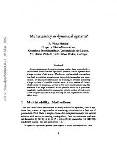
It is mentioned earlier that when a system is quenched from a homogeneous high temperature disordered state to a low temperature state it does not order instantaneously. Broken symmetry phases compete each other to select the equilibrium state and the domains grow with time. A scale-invariant morphology is developed, i.e., the network of domains is (statistically) independent of time when lengths are rescaled by a single characteristic length scale that typically grows algebraically with time [7, 14]. For the zero temperature dynamics the average domain size D increases in time t as D(t) ∼ t1/z , where z is the dynamical exponent associated with the growth. A typical picture of domain coarsening following a quench to zero temperature is shown in figure 18
2.1.
t1
t2
t3
tf
Figure 2.1: Domain growth with time for two dimensional Ising spin system, after a quench to zero temperature. Here t1 < t2 < t3 < tf . tf is the time counted after the system has reached the equilibrium(all up or all down state for T = 0.
2.3.3
Persistence
Apart from the domain growth phenomenon, another important dynamical behavior that has attracted considerable interest recently is persistence. Persis19
tence is simply the probability that the fluctuating nonequilibrium field does not change sign upto time t [15]. The problem of persistence in spatially extended nonequilibrium systems has recently generated a lot of interest both theoretically [16, 17, 18, 19] and experimentally [21, 22]. Single spin persistence provides a natural counterpart to the survival probability in the realm of many-particle systems. In the context of reaction processes, persistence is equivalent to the survival of immobile impurities and therefore does not provide information about collective properties of the bulk [20]. In Ising model, in a zero temperature quench, persistence is simply the probability that a spin has not flipped till time t and is given by P (t) ∼ t−θ , where θ is called the persistence exponent and is unrelated to any other previously known static or dynamic exponents. Persistence probability is in general nonMarkovian time evolution of a local fluctuating variable, such as a spin from its initial state. The persistence probability is hard to measure in simulations, at nonzero temperature, because one needs to distinguish spin flips due to thermal fluctuations from those due to the motion of interfaces. The prescription for measuring the persistence probability for single spin flip at a finite temperature is given in [23]. Apart from such ‘local′ persistence, one can also study the ‘global′ persistence behaviour by measuring the probability PG (t) that the order parameter does not change its sign till time t [24]. At the critical temperature, the probability that the individual spins will not be flipped till time t has an exponential decay, while
20
the global persistence shows an algebraic decay: PG (t) ∼ t−θG .
2.4
Quenching of nearest neighbour Ising model
The Hamiltonian of the Ising spin model we have considered here is given by equation 2.6, where Si = ±1 and the sum is over all nearest-neighbor pairs of sites hiji. Now we ask the question, what is the fate of the Ising system after a zero temperature quench. In one dimension, a zero temperature quench of the Ising model (with nearest neighbour interactions only) ultimately leads to the equilibrium configuration (Figure 2.2). Here the domain walls approach each other and annihilate, the system goes to its stable state (all up or all down) at very large times.
Figure 2.2: Schematic picture of the zero temperature quenching dynamics of one dimensional nearest neighbour Ising model. The red colour domain is shrinking with time and the domain walls between the red and blue colour spin will annihilate each other to form all up state (with blue colour spins only) after few time steps. In higher dimensions, the system cannot reach the ground state for all initial configurations. In two dimensions, the system can find out the ground state for about 70% cases [25]. In two dimension, on the square lattice, there exist a 21
huge number of metastable states that consists of alternating vertical or horizontal stripes whose widths are all ≥ 2. These arise because in zero-temperature Glauber dynamics, a straight boundary between up and down phases is stable (Figure2.3).
Figure 2.3: Schematic picture to show freezing at the zero temperature Glauber dynamics of two dimensional nearest neighbour Ising model. From the schematic picture 2.3, it is very clear that any spin at the boundary is supported by three neighbouring spins and a reversal of any spin along the boundary increases the energy. However, a stripe of width one is unstable, as there will not be any change of energy due to the flipping of one of the spins in the stripe. In three dimensions the Ising spin system (with nearest neighbour interaction), never reaches the ground state by zero temperature single spin flip Glauber dynamics.
2.4.1
Finite size scaling
It is not possible to reach the thermodynamic limit (means L → ∞) numerically, when we are doing the simulations in computer. We always do our simulations in
22
finite system size, no matter how large. So we need the finite size corrections for getting the results at the thermodynamic limit (L → ∞). In this subsection we shall discuss the theory of finite size scaling of the dynamical exponent z and the persistence exponent θ for the zero temperature quenching dynamics. It is already discussed that domain size D increases in time t as D(t) ∼ t1/z . √ Now as magnetization m ∼ D, so magnetization grows with time as m(t) ∼ t1/2z . Let us consider a Ising spin system of d-dimensional geometry of linear size L with nearest neighbour interaction. The system of spins evolve in time following the Glauber dynamics, lowering the total energy of the configuration in the process. the persistence probability shows a power law form in time, P (t) ∼ t−θ , as long as t > t∗ , the domain cannot grow any further because of the finite system size and persistence probability stops decaying, attaining a limiting value P (∞, L) ∼ L−zθ . From the above behaviour of the persistence probability one can write down the dynamical scaling relation [26] P (t, L) ∼ t−θ f (L/t1/z ),
(2.8)
where the scaling function f (x) ∼ x−α with α = zθ for x 1 on the other hand, although the system reaches the ground state at long times, the dynamical exponent and the persistence exponent are both different from those of the Ising model with only nearest neighbour interaction [9]. The above observations and the additional fact that even in the two dimensional nearest neighbour Ising model, frozen-in striped states appear in a zero temperature quench [3], suggest that the two dimensional Ising model in presence of competing interactions could show novel dynamical behaviour. In the present work, we have introduced such an interaction (along one direction) in the two dimensional Ising model, thus making it equivalent to the ANNNI model in two dimensions precisely. The Hamiltonian for the two dimensional ANNNI model on
31
a L × L lattice is given by H = −J0
L X
i,j=1
Si,j Si+1,j − J1
X
[Si,j Si,j+1 − κSi,j Si,j+2].
(3.2)
i,j=1
Henceforth, we will assume the competing interaction to be along the x (horizontal) direction, while in the y (vertical) direction, there is only ferromagnetic interaction. Although the thermal phase diagram of the two dimensional ANNNI model is not known exactly, the ground state is known and simple. If one calculates the magnetization along the horizontal direction only, then for κ < 0.5, there is ferromagnetic order and antiphase order for κ > 0.5. Again, κ = 0.5 is the fully frustrated point where the ground state is highly degenerate. On the other hand, there is always ferromagnetic order along the vertical direction. In Fig. 3.1, we have shown the ground state spin configurations along the x direction for different values of κ.
Highly degenerate
Ferro
Antiphase
++++++ 0
++ −−++ −− 0 .5
κ
T = 0 Figure 3.1: The ground state (temperature T = 0) spin configurations along the x direction are shown for different values of κ. In the ferromagnetic phase, there is a two fold degeneracy and in the antiphase the degeneracy is four fold. The ground state is infinitely degenerate at the fully frustrated point κ = 0.5. In section 3.2, we have given a list of the quantities calculated. In section 3.3, we discuss the dynamic behaviour in detail. In order to compare the results with those of a model without competition, we have also studied the dynamical fea-
32
tures of a two dimensional Ising model with ferromagnetic next nearest neighbour interaction, i.e., the model given by eq. (3.2) in which κ < 0. These results are also presented in section 3.3. Discussions and concluding statements are made in the last section of this chapter.
3.2
Quantities calculated
We have estimated the following quantities in the present work: 1. Persistence probability P (t): As already mentioned, this is the probability that a spin does not flip till time t. In case the persistence probability shows a power law form, P (t) ∼ t−θ , one can use the finite size scaling relation [12] P (t, L) ∼ t−θ f (L/t1/z ).
(3.3)
For finite systems, the persistence probability saturates at a value L−α at large times. Therefore, for x 1. 3. Distribution P (fD ) (or P (ND )) of the fraction (or number) of domain walls at steady state: this is also done for both x and y directions. 4. Distribution P (m) of the total magnetization at steady state for κ ≤ 0 only. We have taken lattices of size L × L with L = 40, 100, 200 and 300 to study the persistence behaviour and dynamics of the domain walls of the system and averaging over at least 50 configurations for each size have been made. For estimating the distribution ND we have averaged over much 34
larger number of configurations (typically 4000) and restricted to system sizes 40 × 40, 60 × 60, 80 × 80 and 100 × 100. Periodic boundary condition has been used in both x and y directions. J0 = J1 = 1 has been used in the numerical simulations.
3.3
Detailed dynamical behaviour
Before going in to the details of the dynamical behaviour let us discuss the stability of simple configurations or structures of spins which will help us in appreciating the fact that the dynamical behaviour is strongly dependent on κ.
3.3.1
Stability of simple structures
An important question that arises in dynamics is the stability of spin configurations - it may happen that configurations which do not correspond to global minimum of energy still remain stable dynamically. This has been termed “dynamic frustration” [13] earlier. A known example is of course a striped state occurring in the two or higher dimensional Ising models which is stable but not a configuration which has minimum energy. In ANNNI model, the stability of the configurations depend very much on the value of κ. It has been previously analysed for the one dimensional ANNNI model that κ = 1 is a special point above and below which the dynamical behaviour changes completely because of the stability of certain structures in the system. Let us consider the simple configuration of a single up spin in a sea of down spins. Obviously, it will be unstable as long as κ < 2. For κ > 2, although this spin is stable, all the neighbouring spins are unstable. However, for κ < 2, only the up spin is unstable and the dynamics will stop once it flips. When κ = 2 the spin may or may not flip, i.e., the dynamics is stochastic. 35
Next we consider a domain of two up spins in a sea of down spin. These two may be oriented either along horizontal or vertical direction. These spins will be stable for κ > 1 only while all the neighouring spins are unstable. For κ < 1, all spins except the up spins are stable. When κ = 1, the dynamics is again stochastic.
−−−−− −−+−− −−−−−
−−−−−− −−++−− −−−−−−
(a)
(b)
−−−−−− −−++−− −−++−− −−−−−− (c) Figure 3.3: Analysis of stability of simple structures: (a) single up spin in sea of down spins; here for κ < 2 all the spins except the up spin is stable (b) two up spins in a sea of down spins, all spins except the two up spins are stable for κ < 1 (c) a two by two structure of up spins - here all the spins are stable for κ < 1 while neighbouring spins are not (see text for details). A two by two structure of up spins in a sea of down spins on the other hand will be stable for any value of κ > 0. But the neighbouring spins along the vertical direction will be unstable for κ ≥ 1. This shows that for κ < 1, one can expect that the dynamics will affect the minimum number of spin and therefore the dynamics will be slowest here. A picture of the structures described above are shown in Fig 3.3. One can take more complicated structures but the analysis of these simple 36
ones is sufficient to expect that there will be different dynamical behaviour in the regions κ < 1, κ = 1, κ > 1, κ = 2 and κ > 2. However, we find that as far as persistence behaviour is concerned, there are only three regions with different behaviour: κ < 1, κ = 1 and κ > 1. On the other hand, when the distribution of the number of domain walls in the steady state is considered, the three regions 1 < κ < 2, κ = 2 and κ > 2 have clearly distinct behaviour.
3.3.2
0 1. In this subsection we discuss the behaviour for κ > 1 while the κ = 1 case is discussed in the next subsection. The persistence probability follows a power law decay with θ = 0.235±0.001 for all κ > 1, while the finite size scaling analysis made according to (3.3) suggests a z value 2.08±0.01. This is checked for different values of κ (κ = 1.3, 1.5, 2.0, 20, 100) and the values of θ and z have negligible variations with κ which do not show any systematics. Hence we conclude that the exponents are independent of κ for κ > 1. A typical behaviour of the raw data as well as the data collapse is shown in Fig. 41
3.10. The dynamics of the average fraction of domain walls along the horizontal direction, fDx again shows a fast saturation while that in the y direction has a power law decay with an exponent ≃ 0.48 (Fig. 3.11). This exponent is also independent of κ. As mentioned in section II, we find that there is a good agreement of the value of this exponent with that of 1/z obtained from the finite size scaling behaviour of P (t) implying that the average domain size D is inversely proportional fDy . This is quite remarkable, as the fraction of domain walls calculated in this manner is not exactly equivalent to the inverse of domain sizes in a two dimensional lattice; the fact that fDx remains constant may be the reason behind the good agreement (essentially the two dimensional behaviour is getting captured along the dimension where the number of domain walls show significant change in time). Although the persistence and dynamic exponents are κ independent, we find that the distribution of the number of domain walls has some nontrivial κ dependence. Though the system, for all κ > 1, evolves to a state with antiphase order along the horizontal direction, the ferromagnetic order along vertical chains is in some cases separated by one or more domain walls. A typical snapshot is shown in Fig. 3.13 displaying that one essentially gets a striped state here like in the two dimensional Ising model. Interfaces which occur parallel to the y axis, separating two regions of antiphase and keeping the ferromagnetic ordering along the vertical direction intact, are extremely rare, the probability vanishing for larger sizes. Quantitatively this means we should get fDx = 0.5 at long times which is confirmed by the data (Fig. 3.11). Hence in the following our discussions on striped state will always imply flat horizontal interfaces, i.e., antiphase ordering along each horizontal row but 42
the ordering can be of different types (e.g., a + + − − + + − − · · · type and a − − + + − − + + · · · type, which one can call a ‘shifted’ antiphase ordering with respect to the first type). It is of interest to investigate whether these striped states survive in the infinite systems. To study this, we consider the distribution of the number of domain walls rather than the fraction for different system sizes. The probability that there are no domain walls, or a perfect ferromagnetic phase along the vertical direction, turns out to be weakly dependent on the system sizes but having different values for different ranges of values of κ. For 1 < κ < 2, it is ≃ 0.632, for κ = 2.0, it is ≃ 0.544 while for any higher value of κ, this probability is about 0.445. Thus it increases for κ although not in a continuous manner and like the two dimensional case, we find that there is indeed a finite probability to get a striped state. While we look at the full distribution of the number of domain walls at steady state (Fig. 3.12), we find that there are dominant peaks at NDy = 0 (corresponding to the unstripped state) and at NDy = 2 (which means there are two interfaces). However, we find that the distribution shows that there could be odd values of NDy as well. This is because the antiphase has a four fold degeneracy and the and a ‘shifted’ ordering can occur in several ways such that odd values of NDy are possible. In any case, the number of interfaces never exceeds NDy = 6 for the system sizes considered.
3.3.4
κ=1
Here we find that the persistence probability follows a power law decay with θ = 0.263 ± 0.001. The finite size scaling analysis suggests a z value 1.84 ± 0.01 (Fig. 3.14). We have again studied the dynamics of fDx and fDy ; the former shows a fast
43
L = 40 L = 100 L = 200 L = 300
P(t)
P(L,t)/t-Θ
100
10-1 10-2 0 10
102 103
106
t 100
κ > 1
10-1
10-1 10-1
100
101
102
L/t1/z
103
Figure 3.10: The collapse of scaled persistence data versus scaled time using θ = 0.235 and z = 2.08 is shown for different system sizes for κ > 1. Inset shows the unscaled data.
No of Domain Walls
100 fD
x
10-1
10-2
10-3 101
fD
y
102
103
104
105
106
Time Figure 3.11: Decay of the fraction of domain walls with time at κ > 1 are shown along horizontal and vertical directions. The dashed line has slope equal to 0.48.
44
0.7
κ > 2.0 κ = 2.0 1.0 < κ< 2.0
Probability of occurence
0.6 0.5 0.4 0.3 0.2 0.1 0 0
1
2
3 4 No. of domain Walls
5
6
Figure 3.12: Normalized steady state distributions of number of domain walls for different κ > 1 show that striped states occur with higher probability as κ increases. The lines are guides to the eye.
40
35
30
25
20
15
10
5
0 0
5
10
15
20
25
30
35
40
Figure 3.13: A typical snapshot of a steady state configuration for κ > 1 with flat horizontal interfaces separating two regions of antiphase ordering (see text).
45
P(t)
P(L,t)/t-Θ
10
L = 40 L = 100 L = 200 L = 300
0
10-1 10-2 100
102 103
106
t 100
κ = 1
10-1
10-1 10-2
10-1
100
101
L/t1/z
102
103
Figure 3.14: The collapse of scaled persistence data versus scaled time using θ = 0.263 and z = 1.84 is shown for different system sizes at κ = 1. Inset shows the unscaled data. saturation at 0.5 while the latter shows a rapid decay to zero after an initial power law behaviour with an exponent ≈ 0.515 (Fig. 3.15). This value, unlike in the case κ > 1, does not show very good agreement with 1/z obtained from the finite size scaling analysis. We will get back to this point in the next section. The results for fDx and fDy imply that the system reaches a perfect antiphase configuration as there are no interfaces left in the system with fDx = 0.5 and fDy = 0 at later times.
3.3.5
κ ≤ 0.0
In order to make a comparison with the purely ferromagnetic case, we have also studied the Hamiltonian (3.2) with negative values of κ which essentially corresponds to the two dimensional Ising model with anisotropic next nearest neighbour ferromagnetic interaction. κ = 0 corresponds to the pure two dimensional Ising model for which the numerically calculated value of θ ≃ 0.22 is verified. We find a new result when κ 46
100 fD
x
10-1 10-2
fD
y
10-3 10-4 10-5 10-6 0 10
101
102
103
104
105
Time
Figure 3.15: Decay of the fraction of domain walls with time at κ = 1 are shown along horizontal and vertical directions. The dashed line has slope equal to 0.515. is allowed to assume negative values, the persistence exponent θ has a value ≃ 0.20 for |κ| > 1 while for 0 < |κ| ≤ 1, the value of θ has an apparent dependence on κ, varying between 0.22 to 0.20. However, it is difficult to numerically confirm the nature of the dependence in such a range and we have refrained from doing it. At least for |κ| >> 1, the persistence exponent is definitely different from that of at κ = 0. The growth exponent z however, appears to be constant and ≃ 2.0 for all values of κ ≤ 0. A data collapse for large negative κ is shown in Fig. 3.16 using θ = 0.20 and z = 2.0. The effect of the anisotropy shows up clearly in the behaviour of fDx and fDy as functions of time (Fig. 3.17). For κ = 0, they have identical behaviour, both reaching a finite saturation value showing that there may be interfaces generated in either of the directions (corresponding to the striped states which are known to occur here). As the absolute value of κ is increased, fDx shows a fast decay to zero while fDy attains a constant value. The saturation value attained by fDy increases markedly with |κ| while for fDx the decay to zero becomes faster. One can conduct a stability analysis for striped states to show that such states become 47
4
P(t)
P(L,t)/t-Θ
L = 100 L = 200 L = 300
0.1 102
103
106
t
1
κ < 0
0.4 0.1
1
L/t1/z
10
100
Figure 3.16: The collapse of scaled persistence data versus scaled time using θ = 0.20 and z = 2.0 is shown for different system sizes for κ < −1. Inset shows the unscaled data. unstable when the interfaces are vertical and κ increases beyond 1, leading to the result fDx → 0. Extracting the z value from the variations of fDx or fDy is not very simple here as the quantities do not show smooth power law behaviour over a sufficient interval of time. The fact that fDy and/or fDx reach a finite saturation value indicates that striped states occur here as well. The behaviour of fDx and fDy suggests that in contrast to the isotropic case where interfaces can appear either horizontally or vertically, here the interfaces appear dominantly along the x direction as κ is increased. Thus the normalized distribution of the number of domain walls along y is shown in Fig. 3.18. We find that as κ is increased in magnitude, more and more interfaces appear. However, the number of interfaces is always even consistent with the fact that interfaces occur between ferromagnetic domains of all up and all down spins. Lastly in this section, we discuss the behaviour of the magnetization which is
48
10-1
fraction of domain walls
κ = -1.5 κ = -1.0 κ = -0.7
10-2
κ = 0.0
κ = 0.0 κ = -0.7
-3
10
κ = -1.0 κ = -1.5 -4
10
101
102
103
104
105
106
Time
Figure 3.17: Decay of the fraction of domain walls with time at κ ≤ 0 are shown along horizontal (fDx ), shown by dotted lines) and vertical (fDy ), shown by solid lines) directions.
0.8
κ = 0.0 κ = -0.7 κ = -1.0 κ = -1.5 κ = -2.0 κ = -20.0
Probability of occurence
0.7 0.6 0.5 0.4 0.3 0.2 0.1 0 0
1
2
3 4 5 No. of domain walls
6
7
8
Figure 3.18: Normalized steady state distributions of number of domain walls for different κ ≤ 0 show that striped states occur with higher probability as |κ| increases. The lines are guides to the eye.
49
the order parameter in a ferromagnetic system. As striped states are formed, the magnetization will assume values less than unity. The probability of configurations with magnetization equal to unity shows a stepped behaviour, with values changing at |κ| = 1 and 2 and assuming constant values at 1 < |κ| < 2 and above
Probability of magnetisation = 1
|κ| = 2 (Fig. 3.19). 0.7 0.6 0.5 0.4 0.3 0.2 0.1 0 -2.5
-2
-1.5
-1
-0.5
0
κ
Figure 3.19: Probability that the magnetization takes a steady state value equal to unity is shown against κ when κ ≤ 0.
3.4
Discussions and Conclusions
We have investigated some dynamical features of the ANNNI model in two dimensions following a quench to zero temperature. We have obtained the results that the dynamics is very much dependent on the value of κ, the ratio of the antiferromagnetic interaction to the ferromagnetic interaction along one direction. This is similar to the dynamics of the one dimensional model studied earlier, but here we have more intricate features, e.g., that of the occurrence of quasi frozen-in structures for κ < 1 where the persistence probability shows a very slow decay with time. Persistence probability is algebraic for κ ≥ 1, but exactly at κ = 1, the exponents θ and z are different from those at κ > 1. The exponents for κ > 1 are 50
in fact very close to those of the two dimensional Ising model with nearest neighbour ferromagnetic interaction. (This was not at all true for the one dimensional ANNNI chain, where the persistence exponent at κ > 1 was found to be appreciably different from that of the one dimensional Ising chain with nearest neighbour ferromagnetic interaction.) This shows that the ferromagnetic interaction along the vertical direction is able to negate the effect of the antiferromagnetic interaction to a great extent. This is apparently a counter intuitive phenomenon, κ = 0 and κ > 1 having very similar dynamic behaviour while in the intermediate values, the dynamics is qualitatively and quantitatively different. At far as dynamics is concerned, the ANNNI model in two dimensions cannot be therefore treated perturbatively. Although the values of θ and z are individually quite close for κ = 0 and κ > 1, the product zθ = α are quite different. For κ = 0, α ≃ 0.44 while for κ > 1, it is 0.486 ± 0.002. This shows that the spatial correlations of the persistent spins are quite different for the two and one can safely say that the dynamical class for κ = 0 and κ > 1 are not the same. κ = 1 is the special point where the dynamic behaviour changes radically. Here there appears to be some ambiguity regarding the value of z; estimating α from the finite size scaling analysis gives α ≈ 0.484 ±0.005 while using the z value from the domain dynamics, the estimate is approximately equal to 0.51. However, the dynamics of the domain sizes may not be very accurately reflected by the dynamics of fDy in which case α ≈ 0.48 is a more reliable result. Thus we find that although the values of θ and z are quite different for κ = 1 and κ > 1, the α values are close. We would like to add here that when there is a power law decay of a quantity related to the domain dynamics, it is highly unlikely that it will be accompanied by an exponent which is different from the growth exponent. Thus, even though we get slightly different values of z for κ = 1 from the two analyses, it is more 51
likely that this is an artifact of the numerical simulations. Another feature present in the two dimensional Ising model is the finite probability with which it ends up in a striped state. The same happens for κ > 1, but here the probabilities are quite different and also dependent on κ. We find that there is a significant role of the point κ = 2 here as this probability has different values at κ = 2, κ > 2 and κ < 2. Comparison of the ANNNI dynamics with that of the ferromagnetic anisotropic Ising model shows some interesting features. In the latter, one gets a new value of persistence exponent for κ < −1 while in the former a new value is obtained for κ ≥ 1.The new values (except for κ = 1) are in fact very close to that of the two dimensional Ising model, but simulations done for identical system sizes averaged over the same number of initial configurations are able to confirm the difference. The qualitative behaviour of the domain dynamics is again strongly κ dependent when κ is negative. Another point to note is that the probability that the system evolves to a pure state is κ dependent in both the ANNNI model and the Ising model. In both cases in fact, this probability decreases in a step like manner with increasing magnitude of κ. We also find the interesting result that while the distribution of the number of domain walls can have non-zero values at odd values of ND in the ANNNI model because of the four fold degeneracy of the antiphase, for the Ising model, odd values of ND are not permissible as the ferromagnetic phase is two fold degenerate. Finally we comment on the fact that although the dynamical behaviour, as far as domains are concerned, reflects the inherent anisotropy of the system (in both the ferromagnetic and antiferromagnetic models), the persistence probability is unaffected by it. In order to verify this, we estimated P (t) along an isolated chain of spins along x and y directions separately and found that the two estimates gave identical results for all values of κ. 52
In conclusion, it is found that except for the region 0 < |κ| < 1, the dynamical behaviour of the Hamiltonian (3.2) is remarkably similar for negative and positive κ; the persistence and growth exponents get only marginally affected compared to the values of the two dimensional Ising case (κ = 0) and the domain distributions have similar nature. However, the region 0 < κ < 1 is extraordinary, where algebraic decay of persistence is absent. There is dynamic frustration as the system gets locked in a metastable state consisting of ladder-like domains and the dynamics is very slow because of the presence of quasi-frozen structures. There is in fact dynamic frustration at other κ values also in the sense that except for κ = 1, the system has a tendency to get locked in a “striped state”. However, even in that case, the algebraic decay of the persistence probability is observed. Thus algebraic decay of persistence probability seems to be valid only when the metastable state is a striped state. Although there is no dynamic frustration at κ = 1 in the sense that it always evolves to a state with perfect antiphase structure, it happens to be a very special point where the persistence exponent and growth exponents are unique and appreciably different from those of the κ = 0 case. In this chapter, the behaviour of the two dimensional ANNNI model under a zero temperature has been discussed; the dynamics at finite temperature can be in fact quite different. At finite temperatures, the spin flipping probabilities are stochastic, and the dynamical frustration may be overcome by the thermal fluctuations. It has been observed earlier [13] that in a thermal annealing scheme of the one dimensional ANNNI model, the κ = 0.5 point becomes significant. A similar effect can occur for the two dimensional case as well. The definition of persistence being quite different at finite temperatures [14], it is also not easy to guess its behaviour (for either the one or two dimensional model) simply from the results of the zero temperature quench. Indeed, the ANNNI model under a finite temperature quench is an open problem which could be addressed in the future. 53
Bibliography [1] J. D. Gunton, M. San Miguel and P. S. Sahni, Phase Transitions and critical phenomena, Vol 8, eds. C. Domb and J. L. Lebowitz (Academic, NY 1983). [2] A. J. Bray, Adv. Phys. 43 357 (1994) and the references therein. [3] V. Spirin, P. L. Krapivsky and S. Redner, Phys. Rev.E 63 036118 (2001). [4] For a review, see S. N. Majumdar, Curr. Sci. 77 370 (1999). [5] B. Derrida, A. J.Bray and C. Godreche, J.Phys. A 27 L357 (1994) [6] D. Stauffer, J. Phys. A 27 5029 (1994). [7] P. L. Krapivsky, E.Ben-Naim and S. Redner, Phys. Rev.E 50 2474 (1994). [8] S. Redner and P. L. Krapivsky, J.Phys. A 31 9229 (1998) [9] P. Sen and S. Dasgupta, J. Phys. A 37 11949 (2004). [10] D. Das and M.S. Barma, Physica A 270 245 (1999); Phys. Rev. E 60, 2577 (1999). [11] W. Selke, Phys. Rep. 170, 213 (1988). [12] G. Manoj and P. Ray, Phys. Rev. E 62 7755 (2000); G. Manoj and P. Ray, J. Phys A 33 5489 (2000). 54
[13] P. Sen and P. K. Das in Quantum Annealing and other optimization problems eds. A. Das and B. K. Chakrabarti, Springer Verlag (2005). [14] B. Derrida, Phys. Rev. E 55 3705 (1997)
55
Chapter 4 Quenching Dynamics: Effect of the nature of randomness of complex networks 4.1
Introduction
The dynamical behaviour of Ising models may change drastically when randomness is introduced in the system. Randomness can occur in many ways and its effect on dynamics can depend on its precise nature. For example, randomness in the Ising model can be incorporated by introducing dilution in the site or bond occupancy in regular lattices and consequently the percolation transition plays an important role [1, 2]. Here the scaling behaviours are completely different from power laws. One can also consider the interactions to be randomly distributed, either all ferromagnetic type or mixed type (e.g., as in a spin glass) [3]; the system goes to a frozen state following a zero temperature quenching in both cases. Another way to introduce randomness is to consider a random field in which case the scaling behaviour is also completely different from power laws [4]. 56
Here we consider Ising models on random graphs or networks where the nearest neighbour connections exist. In addition, the spins have random long range interactions which are quenched in nature. In general, here, the dynamics, instead of leading the system towards its equilibrium state, makes it freeze into a metastable state such that the dynamical quantities attain saturation values different from their equilibrium values. Moreover, rather than showing a conventional power law decay or growth, the dynamical quantities exhibit completely different behaviour in time. A point to be noted here is, when long range links are introduced, the domains are no longer well-defined as interacting neighbours could be well separated in space. This results in freezing of Ising spins on random graphs as well as on small world networks [5, 6]. The phase ordering dynamics of the Ising model on a WattsStrogatz network [7], after a quench to zero temperature, produces dynamically frozen configurations, disordered at large length scales [8, 6]. Even on small world networks, the dynamics can depend on the nature of the randomness; it was observed that while in a sparse network there is freezing, in a densely connected network freezing disappears in the thermodynamic limit [9]. In this chapter, we shall present our investigation on the dynamical behaviour of an Ising system on two different networks following a zero temperature quench. In these two networks, both of which are sparsely connected, the nature of randomness is subtly different and we study whether this difference has any effect on the dynamics. Both these networks are embedded in a one dimensional lattice and the nearest neighbour connections always exist and the nodes have degree four on an average. They differ as in one of the networks, the random long range interactions have a spatial dependence. It may be mentioned here that quenching dynamics on such Euclidean networks has not been considered earlier to the best of our knowledge. 57
It is also quite well known that many dynamical social phenomena can be appropriately mapped to dynamics of spin systems. At the same time, social systems have been shown to behave like complex networks (having small world and/or scale free features etc.). So the present study may be particularly interesting in the context of studying social phenomena described by Ising-type models. In section 4.2.1 we have discussed some basic network properties and network models. In section 4.2.2 we have described the two different networks which we call random model A (RMA) and random model B (RMB). In Section 4.3 we have given a list of the quantities calculated. In section 4.4 and 4.5 we have discussed the detailed dynamical behaviour of Ising spin systems on random model A and random model B respectively. The comparison of the results of the quenching dynamics between the two models are discussed in section 4.6. In addition, a qualitative analysis of the quenching dynamics is also presented. Summary and concluding statements are made in the last section.
4.2
Description of the network models
In this section we shall first discuss some basic network properties and network models as well as the models we have considered for our investigation.
4.2.1
Classification of network models
A network is a set of vertices (nodes) connected via edges (links). Networks with directed edges are called directed networks and those with undirected edges are undirected networks. One may classify the networks studying three basic network properties which are average shortest paths, clustering coefficient and degree distribution. The total number of connections of a vertex is called its degree (k). In a directed network the number of incoming edges of a vertex is 58
called its in-degree ki and the number of outgoing edges is called its out-degree ko . k = ki + ko The clustering coefficient characterize the density of connections in the environment close to a vertex. The clustering coefficient C of a vertex is the ratio between the total number of the edges connecting its nearest neighbours and the total number of all possible edges between all this nearest neighbours. The shortest path length is the shortest distance S between any two nodes (say, A and B ) is the number of edges on the shortest path from A to B through connected nodes. Networks are the same as graphs. In graph theory nodes are termed as vertices and links as edges. Mathematicians had already classified graphs into two groups : 1. Regular graph : In which each vertex is linked to its k nearest neighbours. For regular graph the shortest path distance S ∼ l, where l is the linear dimension of the graph/lattice and clustering coefficient C ∼ 1 (finite). 2. Random graph : In which any two vertices have a finite probability to get linked [10, 11]. So in general in a random graph/network each vertex get linked to k arbitrary vertices. In this network or graph, both D, the diameter of the network (the largest of the shortest distances S) and hSi were found to vary as log(N). It may be mentioned here that in the random graph the degree distribution function P (k) is given by : P (ki = k) =N −1 Ck pk (1 − p)N −k−1 ,
(4.1)
which is basically Binomial distribution, where N = total number of nodes, k = degree of a node. For large N the above equation can be replaced by Poisson distribution : P (k) =
e−hki hkik e−pN (pN)k = k! k!
59
(4.2)
where average degree of graph hki = p(N − 1) ≃ pN The significance of hki lies in the fact of forming cluster in random graphs. Now we would like to introduce two types of network namely (1) small world network and (2) scale free network. 1. Small world Network : It is basically intermediate between the previous two networks. In simple terms this describe the fact that despite huge physical size of real networks, any two nodes are connected by relatively short paths, hence the network is named as ‘small world′. These networks are characterized by large clustering coefficient compared to the corresponding random graph and logarithmic dependence of shortest path [10, 11]. Ssw ∼ log(l) → similar to random graph. Csw ∼ 1 → similar to regular graph. 2. Scale free network : For this type of network, the probability that a node was connected to k other nodes is proportional to k −n . This means their degree distribution follows a power law for large k. In general but not necessarily, scale free networks have small world properties. However the clustering coefficient of the SF model decreases with the network size following approximately a power-law. The decay is slower than the decay observed for random graphs (C = hkiN −1 ) and is also different from the behavior of the small-world models, where C is independent of N [10, 11].
4.2.2
Network models of our interest
The two network models under consideration were introduced in reference [12]. The random model A (RMA) is in fact very similar to the Watts-Strogatz network [7]. Here initially a spin is connected to its four nearest neighbours and then only the second nearest neighbour links are rewired with probability p (Fig. 4.1). In
60
the RMB, each spin is connected to its two nearest neighbour and then two extra bonds (on an average) are attached randomly to each spin. The extra bonds are attached to spins located at a distance l > 1 with probability P (l) ∝ l−α (Fig. 4.1). We keep the first neighbours intact in both cases to ensure that the networks are connected. Average degree per node is four in both the networks. The dynamical evolution is considered on the static networks after the process of rewiring/addition of links is completed (for a review on spatial networks see [13]). REGULAR
01
11 00
01
NETWORK
01
11 00
RANDOM MODEL
0110
11 00 00 11
11 00 00 11
p
11 00 00 11
0110
0110
RANDOM MODEL
B l −α
l−α
0110
11 00
A
P
0110
11 00
11 00 00 11
0110
0110
l −α
11 00 00 11
11 00 00 11
11 00 00 11
Figure 4.1: (Color online) Schematic diagram for different network models. Average degree is 2K = 4 in each network. In the regular network both the first and second nearest neighbours are present. In random model A only second neighbours are rewired with probability p. In random model B first nearest neighbours are always linked while other nodes are linked with the probability l−α with l ≥ 2. The general form of the Hamiltonian in a one dimensional Ising spin system for RMA and RMB can be written as
H =−
X
Jij Si Sj ,
(4.3)
i 0, the nature of RMA is small world like [7, 12]. Euclidean models of RMB type have been studied in a few earlier works [14, 15, 16, 12]. While it is more or less agreed that for α ≤ 1, the network is random and for α > 2, it behaves as a regular network, the nature of the network for intermediate values of α is not very well understood. According to the earlier studies [14, 15, 16, 12], it may either have a small world characteristic or behave like a finite dimensional lattice. In the present work, we assume that RMB has random nature for α < 1 and for 1 < α < 2, it is small world like (at least for the system sizes considered here) following the results of [12], which is based on exact numerical evaluation of shortest distance and clustering coefficients. This is also because the Euclidean model considered in [12] is exactly identical to RMB with average degree four, while the average degree of the Euclidean models considered in the other earlier studies is not necessarily equal to four. In case of RMA, the network is regular and random for only two extreme values p = 0 and p = 1 respectively, whereas for RMB, the random and regular behaviour of the network are observed over an extended region. The regular network corresponding to these two models is the one dimensional Ising spin system with nearest neighbour and next nearest neighbour interactions. We have studied the zero temperature quenching dynamics for this model also, and the results for the dynamics are identical to that of the nearest neighbour Ising spin model. So it will be interesting to note how the dynamics is affected by the introduction of randomness in the Ising spin system and also how the difference in the nature of randomness of the two models RMA and RMB shows up in the dynamics. 62
In the simulations, single spin flip Glauber dynamics is used in both cases, the spins are oriented randomly in the initial state. We have taken one dimensional lattices of size L with 100 ≤ L ≤ 1500 to study the dynamics. The results are averaged over (a) different initial configurations and (b) different network configurations. For each system size the number of networks considered is fifty and for each network the number of initial configuration is also fifty. Periodic boundary condition has been used.
4.3
Quantities Calculated
We have estimated the following quantities in the present work. 1. Magnetization m(t): For a Ising spin system with regular connections and having only the ferromagnetic interaction, the order parameter is usually the magnetization, m =
|
P
i
L
Si |
. L is the size of the system. Magnetization
can be considered as the order parameter, even when the connections are random. We have calculated the growth of magnetization with time and also the variation of the saturation value of the magnetization, msat , with p and α for RMA and RMB respectively. 2. Persistence probability P (t): As already mentioned, this is the probability that a spin does not flip till time t. 3. Energy E(t): In these networks, domain wall measurement is not very significant, as domains are ill-defined. The presence of domain walls in regular lattices causes an energy cost [8]. So instead of the number of domain walls, the appropriate measure for disorder is the residual energy per spin ε = E − E0 = E + 4, where E0 = −4 is the known ground state energy per
63
spin and E is the energy of the dynamically evolving state. In fact, the magnetization is not a good measure of the disorder either, since even when the energy is close to the ground state, magnetization may be very close to zero (this is also true for the models without randomness). So residual energy measurement is the best way to find out whether the system has reached the equilibrium ground state or it is stuck in a higher energy nonequilibrium steady state. We have measured the decay of residual energy ε with time and the variation of its saturation value, εsat , with p and α for RMA and RMB respectively. 4. Freezing probability: The probability with which any configuration freezes, i.e., does not reach the ground state (the state with magnetization m = 1 or the state with zero residual energy) is defined as the freezing probability. 5. Saturation time : It is the time taken by the system to reach the steady state. It has been observed in some earlier studies [17] that it also shows a scaling behaviour with the system size with the dynamical exponent z. This in fact provides an alternative method to estimate z when straight forward methods fail. Both magnetization and energy are regarded as dimensionless quantities (ǫ and E scaled by J) in this work.
4.4
Detailed results of quenching dynamics on RMA
The results of a zero temperature quench for the Ising model on the RMA are presented in this section. Starting from a initial random configuration following a
64
quench to zero temperature the system cannot reach the ground state (the state with zero residual energy) always for any p 6= 0. The magnetization, energy, persistence all attain a saturation value in time. The saturation values of all the quantities show nonmonotonic behaviour as a function of p. Figure 4.2 shows the decay of residual energy per spin and the growth of magnetization with time for different values of the rewiring probability.
p=0.042,L=1000 p=0.099,L=1000 p=0.612,L=1000 p=0.9,L=1000
0.7
1
m(t)
ε(t)
2
p=0.042,L=1000 p=0.099,L=1000 p=0.612,L=1000 p=0.9,L=1000
1
0.4 0.3
0.5
0.2
0.3 0.2
0.1
0.1
1
10
2
10
3
10
4
10
t
1
10
2
10
3
10
4
10
t
Figure 4.2: (Color online) Decay of residual energy per spin and the growth of magnetization with time for RMA for different probabilities. It is to be noted that the dynamic quantities do not show any obvious power law behaviour beyond a few time steps. For small p, there is apparently a power law behaviour for a larger range of time which we believe is the effect of the p = 0 point where such a scaling definitely exists. The saturation value of the residual energy per spin εsat increases with the rewiring probability p (for small p), reaches a maximum for an intermediate value of p (p < 1) and then decreases again. This implies that the disorder of the spin system is maximum for a non trivial value of p = pmaxdis , which can be termed as the point of maximum disorder. The saturation value of magnetization on 65
the other hand decreases for small p and takes its minimum value for another intermediate value of p (p < 1), and then increases again (Fig. 4.3). 1 0.9 εsat,L=1000 εsat,L=800 εsat,L=600 msat,L=1000 msat,L=800 msat,L=600
0.7
0.5
0.3
0.1 0.2
0.4
0.6
0.8
1
p
Figure 4.3: (Color online) Saturation value of residual energy per spin εsat and the saturation value of magnetization msat is plotted with the probability of rewiring p for Random Model A. pmaxdis increases with the system size L for small L and then appears to saturate for larger system sizes. The value of the residual energy at pmaxdis also increases with the system size (Fig. 4.4). This establishes the existence of the point of maximum disorder at an intermediate value of p (p ≃ 0.62) even in the thermodynamic limit. Magnetization reaches a minimum at a value of p which is less than pmaxdis . This implies that there exists a region where both magnetization and energy increase as p increases. This is also apparent from Fig 4.3. The physical phenomena responsible for this intriguing feature is conjectured and discussed in detail in section 4.6.2. The saturation time decreases very fast with the rewiring probability p for small p and remains almost constant as p increases (Fig. 4.5). It is known that for p = 0 the saturation time varies as L2 , here it appears that for any p > 0, 66
RMA
0.62
Residual energy
pmaxdis
0.6
0.58
0.56
0.54
1 0.9 0.8 0.7 200 600 1000 System size (L)
0.52
0.5 200
400
600
800
1000
System size (L)
Figure 4.4: (Color online) Rewiring probability at the point of maximum disorder is plotted with the system size. Inset shows the increase of residual energy at the point of maximum disorder with the increment of the system size. there is no noticeable size dependence. For RMA, the freezing probability is almost unity for small p. However, when the disorder is increased beyond p ≃ 0.5, the freezing probability shows a rapid decrease (Fig: 4.5, inset). In one dimension, we checked that the freezing probability is zero for the regular network (p = 0), but here we find that even for very small values of p, the freezing probability is unity. So there is a discontinuity in the freezing probability at p = 0. This also supports the fact that any finite p can make the dynamics different from a conventional coarsening process. An interesting observation may be made about the behaviour of the saturation value of the residual energy in the region p < 0.5. If one allows p to decrease from 0.5 to 0, the saturation value of the residual energy also decreases although the freezing probability is unity in the entire region. This implies that in this range of the parameter, although the system does not reach the real ground state in any realization of the network (or initial configuration), such that ǫ 6= 0 in each case, the system has a tendency to approach the the actual ground state monotonically with p for p < 0.5 (Fig. 4.3).
67
12×103
L=1000 L=600
Freezing probability
Satuaration Time
10×103
8×10³
6×10³
4×10³
1 0.8 0.6 0.4 0.1 0.3 0.5 0.7 0.9 p
2×10³
0
0.1
0.3
0.5
0.7
0.9
p
Figure 4.5: (Color online) Time of saturation with the probability of rewiring is plotted for two different sizes for Random Model A. Inset shows the variation of freezing probability with the probability of rewiring for RMA.
100 L=1000, p=0.042 L=1000, p=0.154 1.1 0.9
10
b, L=1000 c, L=1000
0.7 0.5 0.3 0.1
-2
0.3
0.5
0.7
0.9 1
p 0.5
10-3
Psat
P(t)-Psat
10-1
0.4 Psat, L=1000 Psat, L=800 Psat, L=600
0.3 0.2
10-4 100
0.1
0.3
0.5
0.7
0.9 1
p 101
102
Time
103
104
Figure 4.6: (Color online) Decay of P (t)−Psat with time t alongwith the stretched exponential function found to fit its form are shown. The inset in the bottom left shows the variation of the saturation value of persistence Psat with p. The other inset on the top right shows the variation of b and c with p.
68
The persistence probability follows a stretched exponential behaviour with time for any non zero p, fitting quite well to the form P (t) − Psat ≃ a exp(−btc ).
(4.4)
The saturation value of the persistence is Psat , and it does not depend on the system size. Psat changes with the rewiring probability p and there also exists an intermediate value of p where the value of Psat is maximum. b and c vary nonmonotonically with p (Fig. 4.6).
4.5
Detailed results of quenching dynamics on RMB
In this section we will present the results of the zero temperature quenching dynamics of Ising model on RMB. Here also the system does not reach the ground state always for any finite value of α. The magnetization, energy, persistence all attain a saturation value in time as in RMA. Figure 4.7 shows the decay of residual energy per spin and the growth of magnetization with time for different values of α. It is to be noted that the dynamical quantities do not show any obvious power law behaviour also for RMB. The saturation values of all the quantities show nonmonotonic behaviour as a function of α. The saturation value of residual energy per spin εsat increases with α for small α, reaches a maximum for a finite value of α and then decreases again. This implies that for the RMB also, the disorder of the spin system is maximum for a finite value of α, which is the point of maximum disorder here. On the other hand, the saturation value of the magnetization decreases for small α and takes its minimum value for another finite value of α and then slowly increases (Fig. 69
α=0.5,L=1000 α=1.0,L=1000 α=1.2,L=1000 α=3.0,L=1000
2
α=0.5,L=1000 α=1.0,L=1000 α=1.2,L=1000 α=3.0,L=1000
1
m(t)
ε(t)
0.7 1
0.4 0.3
0.5
0.2
0.3 0.2
0.1 0.1
1
10
2
10
3
10
4
10
t
1
10
2
10
3
10
4
10
t
Figure 4.7: (Color online) Decay of residual energy per spin and the growth of magnetization with time for RMB for different probabilities. 4.8). The value of α = αmaxdis , at which the maximum disorder occurs, decreases with the system size L for small L and then saturates for larger system sizes. The value of the residual energy at αmaxdis also increases with the system size (Fig. 4.9). This establishes the existence of the point of maximum disorder, for the RMB, at a finite value of α (α ≃ 1.2) even in the thermodynamic limit. Similar to the RMA, here is a region beyond α = 1.2 where the energy and the magnetization both decrease, until the magnetization starts growing again. As already mentioned, this issue is addressed in section 4.6.2. Saturation time for RMB in the random network in the region 0 ≤ α < 1 shows too large fluctuations to let one conclude whether it is a constant in this region or has a variation with α. Beyond α = 1 and upto α = 3.0, it is almost independent of α. For α > 3 the saturation time increases with α. There is no remarkable finite size effect in the saturation time for the RMB for any finite value of α. The saturation time varies as L2 for a regular lattice corresponding to 70
0.9
εsat,L=1000 εsat,L=800 εsat,L=600 msat,L=1000 msat,L=800 msat,L=600
0.7
0.5
0.3
0.1 0
2
4
6
α
8
Figure 4.8: (Color online) Saturation value of residual energy per spin εsat and the saturation value of magnetization msat is plotted with α for Random Model B.
2 RMB
Residual energy
αmaxdis
1.8
1.6
1.4
0.9 RMB
0.7
0.5 200 600 1000 1500 System size (L)
1.2
1 200
600
1000
1500
System size (L)
Figure 4.9: (Color online) The value of α at the point of maximum disorder is plotted with the system size. Inset shows the increase of residual energy at the point of maximum disorder with the increment of the system size.
71
α → ∞, here it appears that for any finite α, however large, there is no remarkable size dependence. The freezing probability is small for α = 0 (≃ 0.2) and increases rapidly with α for small α. Freezing probability becomes almost unity beyond α ≃ 1.2 and remains the same for large α. It seems that for any finite α > 1.2 freezing probability remains unity and it will be zero only at α → ∞ (Fig. 4.10), as in one dimension, the freezing probability is zero for the regular network. So for RMB there is a discontinuity of freezing probability at α = ∞ which corresponds to the p = 0 point of RMA. 3
12×10
3
10×10
L=1000 L=600
Freezing probability
Satuaration Time
14×10
3
8×10
3
6×10
3
4×10
3
2×10
3
0
1
1 0.8 0.6 0.4 0.2 1 2 3 4 5 6 7 α
2
3
α
4
5
6
7
Figure 4.10: (Color online) Time of saturation with the value of α is plotted for two different sizes for Random Model B. Inset shows the variation of freezing probability with α for RMB. Beyond α ≃ 1.2, the energy decreases with α though the freezing probability remains unity. This implies that although the system definitely reaches a frozen state, it approaches the real ground state monotonically as α → ∞ (Fig. 4.8). The above results indicate that, though for α > 2 the network behaves as a regular one, dynamically the network is regular only at its extreme value α → ∞. We find that the persistence probability follows roughly a stretched exponential form with time (given by equation (2)) for any finite α. The saturation value of 72
the persistence, Psat , does not depend on the system size. Psat changes with α and there exists an intermediate value of α where the value of Psat is maximum. For RMB also b and c vary nonmonotonically with α (Fig: 4.11). 100 L=1000, α=0.5 L=1000, α=1.2 0.5
Psat
P(t)-Psat
10-1 0.4 Psat, L=1000 Psat, L=800 Psat, L=600
0.3
10-2
0
1
3
0.9
10-3
α
5
7
b, L=1000 c, L=1000
0.7 0.5 0.3 0
10
-4
100
1
3
α
101
5
7 102
Time
103
104
Figure 4.11: (Color online) Decay of P (t) − Psat with time t along with the stretched exponential function found to fit it approximately are shown. The inset in the top right shows the variation of the saturation value of persistence Psat with α. The other inset on the bottom left shows the variation of b and c with α.
4.6 4.6.1
Discussions on the results Comparison of the results for RMA and RMB
In the last two sections the results of a quench at zero temperature for the Ising model on RMA and RMB have been presented separately. In this subsection we will compare the results to understand how the difference in the nature of randomness affects the dynamics of Ising spin system. The gross features of the results are similar: in both models we have a freezing effect which makes the system get stuck in a higher energy state compared to the static equilibrium state in which all spins are parallel. No power law scaling 73
behaviour with time is observed in the dynamic quantities in either model. There exists a point in the parameter space where the deviation from the static ground state is maximum. The behaviour of the saturation times and freezing probability as functions of the disorder parameters are also quite similar qualitatively. The saturation values of magnetization and persistence attain a minimum and maximum value respectively at an intermediate value of the relevant parameters in both models. The decay of the persistence probability also follows the same functional form in the entire parameter space. The saturation values of the persistence has no size dependence for both the models. This indicates that as a whole the dynamics is not much affected due to the change in the nature of randomness of the Ising spin system. Let us consider the parameter values at which the RMA and RMB are equivalent as a network: RMA and RMB behave as random networks at p = 1 and α = 0 respectively. So one can expect that the saturation values of residual energy per spin, magnetization and the numerical value of the saturation time would be same at these values. However, the numerical values of these quantities are quite different. For RMA, at p = 1 the saturation value of the residual energy per spin εsat ≃ 0.415 whereas for RMB at α = 0 εsat ≃ 0.224 for L = 1000. Similarly we found numerically that for RMA the value of saturation magnetization msat ≃ 0.735 for RMA and msat ≃ 0.855 for RMB for the same system size. This is because even though the networks are both random here, the connections have a subtle difference. For RMA, the number of second nearest neighbour is exactly zero at p = 1 and all the other long range neighbour connections are equally probable. On the other hand, for RMB, second nearest neighbours can be still present in the network and the probability is same for this and any other longer range connection. This difference in the nature of randomness affects the dynamics of the Ising spin system sufficiently to make the saturation values different. This means 74
that the systems are locked at different nonequilibrium steady states. For RMB, it is closer to the actual ground state as it is more short ranged in comparison. The other values at which the two networks are equivalent are p = 0 and α > 2 where regular network behaviour is found as far as the network properties are concerned. Interestingly, the behaviour of RMB even when α is finite and greater than 2, is not quite like the dynamics of a regular one dimensional lattice with nearest and next nearest neighbour links only. In fact, the point at which the magnetization becomes minimum is well inside the region α > 2 and not within the small world region as in RMA. Actually there is an extended region of regular and random network behaviour for the RMB, and as a result, a few more interesting points are possible to observe here. Only at the extreme point α = ∞, the one dimensional Ising exponents z = 2.0 and θ = 0.375 can be recovered as the frozen states continue to exist even for finite values of α > 2 for RMB. For the regular network with nearest and next nearest neighbour model, we have checked that there is no freezing at all. So discontinuities of the freezing probabilities occur at p = 0 and α = ∞ on RMA and RMA respectively. Though the nature of randomness is different for RMA and RMB, for both the models there exists a point of maximum disorder where the saturation value of the residual energy per spin attains a maximum value. For RMB, maximum disorder of the Ising spin system occurs near the static phase transition point (small world to random phase) whereas for RMA, the point of maximum disorder is well within the small world region. We try to explain this considering the deviation from the point p = 1 (for RMA) and α = 0 (for RMB). Two processes occur simultaneously here: (a) Number of connections with further neighbours decreases and (b) clustering becomes more probable. As a result of these two processes, freezing occurs. For RMA, the effect is less as there is less clustering [12]. But for RMB, the effect is more 75
and spans the entire parameter space α > 1 and therefore the point of maximum disorder of Ising spin system is very close to the random - small world phase transition point α = 1. The question may arise whether this difference prevails when the models are made even more similar. In RMB, the probability p3 (α) that l ≥ 3 can be expressed as a function of α: Pl=L/2
l=3 p3 (α) = Pl=L/2 l=2
l−α l−α
.
(4.5)
A further correspondence between the two networks can be established by imposing p = p3 (α), which makes the number of second neighbour links in RMA and RMB also same (but the rest of the extra links are connected differently). Using equation (3) we can obtain the value of p corresponding to a given value of α and vice versa. But it is immediately seen that the two networks are not equivalent even after making them similar upto the second neighbour connections. For example, for α = 2.0, the corresponding value of p = 0.612 in this scheme. But we have already seen that while the point of maximum disorder occurs close to this value of p in RMA, the point of maximum disorder for RMB is considerably away from α = 2.0. So the nature of randomness continues to affect the dynamics at least quantitatively.
4.6.2
Analysis of some general features of the quenching phenomena on networks
We find several interesting features in the quenching phenomena of Ising spin systems on both the networks and in this subsection we attempt to provide an understanding of the same.
76
It is intriguing that the results indicate that the minimum amount of randomness can make the system freeze. What happens for small randomness? The interactions are still dominantly nearest neighbour type and domains in the conventional sense should grow which will be of both plus and minus signs. The system will freeze as there will be some stable domain walls due to the few long range interactions present. The domains, as the system attains saturation, will be small in number and large in size irrespective of their signs. As a result, the magnetization attains a small value while the residual energy is still small. This effect continues for some time till something more interesting happens. Take for example the case of quenching on RMA. There is a distinct region 0.4 < p < 0.6 where the energy and magnetization grow simultaneously, an apparently counterintuitive result. Similar behaviour can be noted for the quenching on RMB in a certain region in its parameter space. A problem to analyse the situation for different p (or α) values is that the final frozen states are not related in any way in principle. This is because the energy landscapes change as p is changed and the initial configurations which undergo evolution are completely uncorrelated. In fact, in such a situation, even if the energy landscape is same with a number of local minima, different initial configurations will end up in different final nonequilibrium steady states. Nevertheless, one can attempt to explain this counterintuitive result assuming that the final states are not largely different when p is changed slightly in the following way. This assumption and explanation are supported by the actual final states obtained for small system sizes. Let us for example consider the RMA and take two values of p, p2 > p1 , and for which the magnetization and residual energy of the final state corresponding p2 are both larger than those for p1 . Now this can be possible due to the fragmentation of a larger domain into several domains such that the magnetization increases. This can be demonstrated with a simple example: let us imagine a situation where one 77
has only two domains of size N + (of up spins) and N − (of down spins) for p1 with magnetization equal to m1 = |(N + − N − )|/L and assume that for p2 , the domain with N + up spins remains same while the domain with N − down spins gets fragmented into three domains of size N − 1 , N + 1 and N − 2 in the final state. For p2 , therefore, the magnetization is m2 = |(N + +2N + 1 −N − )|/L which is larger than m1 . Here in this hypothetical case, we have assumed that N + > N − , and p2 is very close to p1 . One can also assume that the energy increases for p2 as the system is still sufficiently short ranged and the new domain walls cause an extra energy compared to the state obtained for p1 . Of course this is an oversimplified picture where we have assumed that the final states for p1 and p2 are identical except for the fragmentation of one domain. However, we find that the final configurations obtained for small systems for different values of p as shown in Fig. 4.12 are consistent with our conjecture. These snapshots are representative of the real situation in the sense that they give a typical picture and are not just rare cases; we have obtained a similar picture from almost all such configurations generated for small systems. As p further increases, should the domains get fragmented into even smaller pieces? Answer is no, as the increasing number of long range interactions again help in the growth of so called domains, of one particular sign only such that the magnetization grows and the energy decreases. However, domains of both signs still survive, although the sizes are no longer comparable. It can therefore be expected that the region for which both magnetization and energy increase as a function of p or α would continue till the short range interactions are dominating and our results are consistent with this expectation.
78
p=0.8
p=0.7
p=0.55
p=0.4
0
10
20
30
40
50
60
Sites
Figure 4.12: (Color online) Snap shots of the final spin configurations for different values of the disorder parameter p for quenching on RMA. The + and • signs indicate up and down spins respectively. The domains in the conventional sense are clearly visible.
4.7
Summary and concluding remarks
In this chapter, we addressed the question how the quenching dynamics of Ising spins depend on the nature of randomness of the underlying network by considering two networks in which the randomness is realized differently. The networks are same upto the first neighbour links and have same average degree per node. While the qualitative features are same, there are intricate differences occurring in the behaviour of the saturation values of the dynamical quantities. Overall, we find some interesting features: the saturation values of the dynamical quantities do not have monotonic behaviour as a function of the disorder parameters. Especially, we find that increasing randomness does not necessarily make the system get locked in a higher energy state. The dynamics takes the system to a steady state very fast, and the saturation times are not dependent on the system size. No scaling behaviour is obtained from the studies either with time or with system size for any of the dynamic quantities. The most sur79
prising result is perhaps the existence of a region in the parameter space where both the residual energy and the magnetization increase which can be explained phenomenologically. The Euclidean model, on which the study of the quenching of Ising spins is done for the first time to the best of our knowledge, shows some surprising behaviour both in the random and regular regions. We find that decreasing randomness makes the system end up in a higher energy state in the random region while in the regular region, familiar behaviour of the Ising dynamics with short range interactions are not obtained; in fact the probability of freezing is unity here indicating that in none of the realization, the system could end up in the static ground state. The saturation time also does not show scaling with time. As already mentioned, the present study is relevant for dynamical social phenomena on complex networks. For example, the evolution of binary opinions on a complex network (where the initial states are randomly +1 and −1) is analogous to the dynamical study reported in the present chapter. Of course, in case of the opinion dynamics, the interactions could be more complex compared to the the simple Ising model. Our result indicates that the qualitative features of the results will not be much different for different complex networks. Dynamic frustration [18] is responsible for freezing in many Ising systems where there is no frustration in the conventional sense. One interesting observation is that the nature of dynamic frustration in regular lattices of dimension greater than one and that in systems with random interaction (but no frustration) are in general quite different as in the latter one does not encounter the familiar scaling laws.
80
Bibliography [1] C. K. Harris and R. B. Stinchcombe, Phys. Rev. Lett. 56, 869 (1986). [2] S. Jain, J. Phys A 19 , L57 (1986); S. Jain, Phys. Rev. E 59, R2493 (1999). [3] C. M. Newman, D. L. Stein, Phys. Rev. Lett. 82, 3944 - 3947 (1999). [4] D. S. Fisher, P. L. Doussal and C. Monthus, Rhys Rev E 64, 066107 (2001). [5] P. Svenson, Phys. Rev. E 64 036122 (2001). [6] O. Haggstrom, Physica A 310 275 (2002). [7] D. J. Watts and S. H. Strogatz, Nature 393, 440 (1998). [8] D. Boyer and O. Miramontes, Phys. Rev. E 67, R035102 (2003). [9] P. K. Das and P. Sen, Eur. Phys. J. B 47, 306 (2005). [10] R. Albert, A.-L. Barabsi, Rev. Mod. Phys. 74, 47 (2002) [11] M. E. J. Newman, SIAM Review 45, 167 (2003) [12] S. Goswami, S. Biswas and P. Sen Physica A 390, 972 (2011). [13] M. Barthlemy, Physics Reports, 499, 1 (2011)
81
[14] J. Kleinberg, Nature 406, 845 (2000); S. Jespersen and A. Blumen, Phys. Rev. E 62, 6270 (2000). P. Sen and B. K. Chakrabarti, J. Phys A 34, 7749 (2001). [15] P. Sen, K. Banerjee, T. Biswas, Phys. Rev. E 66 037102 (2002); C. F. Moukarzel and M. A. de Menezes, Phys. Rev. E 65 056709 (2002); P. Sen, K. Banerjee and T. Biswas, Phys. Rev. E 66, 037102 (2002); H. Zhu and Z-X. Huang, Phys. Rev. E 70, 036117 (2004); A. Chatterjee and P. Sen, Phys. Rev. E 74 036109 (2006); YuF. Chang, L. Sun and X. Cai, Phys. Rev. E 76 021101 (2007); [16] For a recent review on Euclidean networks, see P. Sen, in Recent Developments in Theoretical Physics, eds S. Ghosh and G. Kar, World Scientific, Singapore, 2010, p. 375. [17] P. Sen and S. Dasgupta, J. Phys. A 37 11949 (2004); P. Sen, Phys. Rev. E 81, 032103 (2010), S. Biswas and P. Sen, J. Phys. A 44 145003 (2011). [18] P. Sen and P. K. Das, in Quantum Annealing and other optimisation problems, eds. A. Das and B. K. Chakrabarti, Springer Verlag p 325 (2005).
82
Chapter 5 Opinion formation : A newly proposed dynamics 5.1
Introduction
Sociophysics has emerged as one of the important areas of research during recent times. The concepts of statistical physics find application to many situations that occur in a social system with the assumption that individual free will or feelings do not take crucial role in these situations [1, 2]. One of the major issues that has attracted a lot of attention is how opinions evolve in a social system. Starting from random initial opinions, dynamics often leads to a consensus which means a major fraction of the population support a certain cause, for example a motion or a candidate in an election etc. Simulating human behaviour by models effectively implies quantifying the outcome of the behavior by suitable variables having continuous or discrete values. Different dynamical rules are proposed for the evolution of these variables, depending on how these variables change with time following social interactions. Thus, a social system can be treated like a physical system. For example, in case 83
of opinion dynamics, if the opinions have only discrete binary values, the social system can be regarded as a magnetic system of Ising spins. In this context, Schelling model [3], proposed in 1971, seems to be the very first model of opinion dynamics. Since then, a number of models describing the formation of opinions in a social system have been proposed [4]. While on one hand these models attempt an understanding of how a society behaves and social viewpoints evolve, on the other hand, these provide rich complex dynamical physical systems suitable for theoretical studies. Many of these show a close connection to familiar models of statistical physics, e.g., the Ising and the Potts models. Dynamics of complex systems has become a subject of extensive research from several aspects. For many such systems, e.g., traffic or agent based models, one cannot define a conventional Hamiltonian or energy function. The only method by which one can study the steady state behaviour of such systems is by looking at the long time dynamics. Nonequilibrium dynamics involves the evolution of a system from a completely random initial configuration and associated with this evolution are several phenomena of interest like domain growth or persistence that have been studied, for example, in spin systems. Since in many sociophysics model, one can have variables analogous to spin variables, these phenomena can be readily studied here. An important objective is to identify dynamical universality classes by estimating the relevant dynamical exponents. Another point of interest in studying dynamics is that many systems may have identical equilibrium behaviour but behave differently as far as dynamics is concerned. For example, Ising spin dynamics with or without conservation belong to different dynamic universality class although their equilibrium behaviour is identical. Apart from the dynamical behaviour, different kinds of phase transitions have also been observed in these models by introducing suitable parameters. One such 84
phase transition can be from a homogeneous society where everyone has the same opinion to a heterogeneous one with mixed opinions [5]. Change in the opinion of an individual takes place in different ways in different models. For example in the Voter model [6], an individual simply follows the opinion of a randomly chosen neighbour while in the Sznajd model [7], the opinion of one or more individuals are changed following more complicated rules.
5.2
Description of the proposed model
In a model of opinion dynamics, the key feature is the interaction of the individuals. Usually, in all the models, it is assumed that an individual is influenced by its nearest neighbours. In this chapter we propose a one dimensional model of binary opinion in which the dynamics is dependent on the size of the neighbouring domains as well. Here an individual changes his/her opinion in two situations: first when the two neighbouring domains have opposite polarity, and in this case the individual simply follows the opinion of the neighbouring domain with the larger size. This case may arise only when the individual is at the boundary of the two domains. An individual also changes his/her opinion when both the neighbouring domains have an opinion which opposes his/her original opinion, i.e., the individual is sandwiched between two domains of same polarity. It may be noted that for the second case, the size of the neighbouring domains is irrelevant. This model, henceforth referred to as Model I, can be represented by a system of Ising spins where the up and down states correspond to the two possible opinions. The two rules followed in the dynamical evolution in the equivalent spin model are shown schematically in Fig. 5.1 as case I and II. In the first case the spins representing individuals at the boundary between two domains will choose the opinion of the left side domain (as it is larger in size). For the second case the 85
down spin flanked by two neighbouring up spins will flip.
Case−I
Case−II
Figure 5.1: Dynamical rules for Model I: in both cases the encircled spins may change state; in case I, the boundary spins will follow the opinion of the left domain of up spins which will grow. For case II, the down spin between the two up spins will flip irrespective of the size of the neigbouring domains. The main idea in Model I is that the size of a domain represents a quantity analogous to ‘social pressure’ which is expected to be proportional to the number of people supporting a cause. An individual, sitting at the domain boundary, is most exposed to the competition between opposing pressures and gives in to the larger one. This is what happens in case I shown in Fig.5.1. The interaction in case II on the other hand implies that it is difficult to stick to one’s opinion if the entire neighbourhood opposes it. Defining the dynamics in this way, one immediately notices that case II corresponds to what would happen for spins in a nearest neighbour ferromagnetic Ising model (FIM) in which the dynamics at zero temperature is simply an energy minimisation scheme. However, the boundary spin in the FIM behaves differently in case I; it may or may not flip as the energy remains same. In the present model, the dynamics is deterministic even for the boundary spins (barring the rare instance when the two neighbourhoods have the same size in which case the individual changes state with fifty percent probability). In this model, the important condition of changing one’s opinion is the size of the neighbouring domains which is not fixed either in time or space. This 86
is the unique feature of this model, and to the best of our knowledge such a condition has not been considered earlier. In the most familiar models of opinion dynamics like the Sznajd model [7] or the voter model [6], one takes the effect of nearest neighbours within a given radius and even in the case of models defined on networks [8], the influencing neighbours may be nonlocal but always fixed in identity.
5.3
Model I : Detailed dynamics
We have done Monte Carlo simulations to study the dynamical evolution of the proposed model from a given initial state. With a system of N spins representing individuals, at each step, one spin is selected at random and its state updated. After N such steps, one Monte Carlo time step is said to be completed. If N+ is the number of people of a particular opinion (up spin) and N− is the number of people of opposite opinion (down spin), the order parameter is defined as m = |N+ − N− |/N. This is identical to the (absolute value of) magnetization in the Ising model. Starting from a random initial configuration, the dynamics in Model I leads to a final state with m = 1, i.e., a homogeneous state where all individuals have the same opinion. It is not difficult to understand this result; in absence of any fluctuation, the dominating neighbourhood (domain) simply grows in size ultimately spanning the entire system. We have studied the dynamical behaviour of the fraction of domain walls D and the order parameter m as the system evolves to the homogeneous state. We observe that the behaviour of D(t) and m(t) are consistent with the usual scaling behaviour found in coarsening phenomena; D(t) ∝ t−1/z with z = 1.00 ± 0.01 and m(t) ∝ t1/2z with z = 0.99 ± 0.01. These variations are shown in Fig. 5.2. 87
L=5000 L=1000 slope=0.51
0
10
10
D
m
0
-1
10 -1 10 -2 10 -3 10 -5
10
0
1
2
3
4
10 10 10 10 10 Time
-2
10
0
10
1
10
2
10
Time
3
10
4
10
Figure 5.2: (Color online) Growth of order parameter m with time for two different system sizes along with a straight line (slope 0.51) shown in a log-log plot. Inset shows the decay of fraction of domain wall D with time. We have also calculated the persistence probability that a person has not change his/her opinion up to time t. Persistence, which in general is the probability that a fluctuating nonequilibrium field does not change sign upto time t, shows a power law decay behaviour in many physical phenomena, i.e., P (t) ∝ t−θ , where θ is the persistence exponent. In that case, one can use the finite size scaling relation [9, 10] P (t, L) ∝ t−θ f (L/t1/z ).
(5.1)
For finite systems, the persistence probability saturates at a value ∝ L−α at large times. Therefore, for x 0 when people do not follow the same opinion any longer. The variation of ms with N shows that ms → 0 in the thermodynamic limit for ρ > 0. Thus not only does the society become heterogeneous at the onset of ρ, it goes to a completely disordered state analogous to the paramagnetic state in magnetic systems. Thus one may conclude that a phase transition from a ordered state with m = 1 to a disordered state (m = 0) takes place for ρ = 0+ . It may be recalled here that m = 0 at the trivial fixed point ρ = 1 and therefore the system flows to the ρ = 1 fixed point for any nonzero value of ρ indicating that ρ = 1 is a stable fixed point. That the saturation values of the fraction of domain walls do not show system size dependence for ρ = 0+ further supports the fact that the phase transition occurs at ρ = 0. The effect of the parameter ρ is therefore very similar to thermal fluctuations in the Ising chain, which drives the latter to a disordered state for any non-zero temperature, ρ = 1 being comparable to infinite temperature. However, the role of the rigid individuals is more similar to domain walls which are pinned rather than thermal fluctuations. In fact, the Ising model will have dynamical evolution even at very high temperatures while in Model II, the dynamical evolution becomes slower with ρ, ultimately stopping altogether at ρ = 1. This is reflected in the scaling of the various thermodynamical quantities with ρ, e.g., the order parameter shows a power law scaling above the transition point. Since the role of ρ is similar to domain wall pinning, one can introduce a depinning probability factor µ which in this system represents the probability for rigid individuals to become non-rigid during each Monte Carlo step. µ relaxes the rigidity criterion in an annealed manner in the sense that the identity of 92
µ=1
µ
ρ=0
+
ρ
ρ=1
Figure 5.6: The flow lines in the ρ − µ plane: Any non-zero value of ρ with µ = 0 drives the system to the disordered fixed point ρ = 1. Any nonzero value of µ drives it to the ordered state (µ = 1, which is a line of fixed points) for all values of ρ. the individuals who become non-rigid is not fixed (in time). If µ = 1, one gets back Model I (identical to Model II with ρ=0) whatever be the value of ρ, and therefore µ = 1 signifies a line of (Model I) fixed points, where the dynamics leads the system to a homogeneous state. With the introduction of µ, one has effectively a lesser fraction ρ′ of rigid people in the society, where ρ′ = ρ(1 − µ).
(5.3)
The difference from Model II is, of course, that this effective fraction of rigid individuals is not fixed in identity (over time). Thus when ρ 6= 0, µ 6= 0, we have a system in which there are both quenched and annealed disorder. It is observed that for any nonzero value of µ, the system once again evolves to a homogeneous state (m = 1) for all values of ρ. Moreover, the dynamic behaviour is also same as Model I with the exponent z and θ having identical values. This shows that the nature of randomness is crucial as one cannot simply replace a system with parameters {ρ 6= 0, µ 6= 0} by one with only quenched randomness {ρ′ 6= 0,
93
µ′ = 0} as in the latter case one would end up with a heterogeneous society. We therefore conclude that the annealed disorder wins over the quenched disorder; µ effectively drives the system to the µ = 1 fixed point for any value of ρ. This is shown schematically in a flow diagram (Fig. 5.6). It is worth remarking that it looks very similar to the flow diagram of the one dimensional Ising model with nearest neighbour interactions in a longitudinal field and finite temperature.
5.5
Mapping of the opinion dynamics model to reaction diffusion system
The opinion dynamics model discussed so far are models where the dynamics is described in terms of the Ising spins that mimic the binary opinions an individual can have. In this model, a spin deep inside a domain does not flip. The dynamics is governed by the flipping of the spins only at the domain walls. The dynamics, in this respect, is reminiscent of the zero temperature Glauber dynamics of the kinetic Ising model. The motions of the domain walls can be viewed as the motions of the particles A with the reaction A + A → ∅. This means the particles are walkers and when two particles come on top of each other they are annihilated. The annihilation reaction ensures domain coalescence and coarsening. Unlike that in Glauber Ising model, the walkers A corresponding to Model I do not perform random walks. These walkers move ballistically towards their nearest neighbours. This bias, as we have seen before, gives rise to a new universality class than that of conventional reaction diffusion system [16]. We have also studied A + A → ∅ model with the particles A performing random walk with a bias ǫ towards their nearest neighbors. We have taken ǫ as the probability that a walker walks towards its nearest neighbour. Clearly, ǫ =
94
0.5 corresponds to usual reaction diffusion system with the particles performing random walk. On the other hand, ǫ = 1 is equivalent to our Model I as has been described above. We have studied the dynamics of the reaction diffusion system for different values of ǫ in the range [0+ , 1.0]. In reaction diffusion systems, the growth of domains is given by the number of surviving walkers. Persistence P (t) in these systems is defined as the fraction of sites unvisited by any of the walkers A till time t. Figures 5.7 and 5.8 show the decay of persistence and fraction of walkers with time for different values of ǫ > 0.5. 1 L=500,ε=0.7 L=1000,ε=0.7 L=1000,ε=0.55 L=500,ε=0.55 slope=-0.23
0.7
Persistence
0.5 0.3
0.1
100
101
102
103
104
105
Time
Figure 5.7: Decay of persistence with time for ǫ = 0.7 and ǫ = 0.55
We find that for ǫ > 0.5, the Model I behaviour is observed, namely: z ≃ 1.0 and θ ≃ 0.235, with some possible correction to the scaling which becomes weaker as ǫ is increased. For example, there is a logarithmic correction to scaling for the decay of the fraction of domain walls which takes the form t−1 (1 + α(ǫ) log(t)) where α(ǫ) → 0 as ǫ → 1. One can compare the above model with the cases discussed in section 2.2.3, where the introduction of stochastic dynamics also 95
occurred with a bias towards the larger domain. In case of thermal disorder, the parameter comparable to ǫ is β. In the present case, the exact sizes of the domains do not matter (which is important for the case with β) but the results are consistent in the sense that any bias towards the larger domain (or nearest walker) makes the system behave like Model I.
Fraction of walkers
100
L=500,ε=0.7 L=1000,ε=0.7 L=1000,ε=0.55 L=500,ε=0.55 slope=-1.0 f(t)
10-1
10-2
10-3
100
101
102
103
104
105
Time
Figure 5.8: Decay of number of walkers with time for ǫ = 0.7 and ǫ = 0.55. There is a logarithmic correction to scaling for the value of ǫ = 0.55. The form of f (t) is t−1 (1 + α log(t)) with α = 3.92
In this model, we have also studied the ǫ < 0.5 region where the opposite happens, the walker has a bias towards the further neighbour. Obviously domain annihilations take place very slowly now, even slower than 1/ log(t) and the dynamics continues for very long times. Consequently, the persistence probability no longer shows a power law variation now but falls exponentially to zero (Fig 5.9).
96
100
Dw(t)*0.4,ε=0.3 Dw(t)*0.4,ε=0.45 P(t),ε=0.45 P(t),ε=0.3 g(t)
10-1
10-2
10-3
10-4 0 10
101
102
103
104
105
Time
Figure 5.9: Decay of persistence and number of walkers with time for ǫ = 0.3 and ǫ = 0.45. The form of g(t) is a(1/ log(t)) where a is any constant.
5.6
Summary and concluding remarks
In summary, we have proposed a model of opinion dynamics in which the social pressure is quantified in terms of the size of domains having same opinion. In the simplest form, the model has no disorder and self organises to a homogeneous state in which the entire population has the same opinion. This simple model exhibits novel coarsening exponents. This model (Model I) in one dimension belongs to a new dynamical universality class with novel dynamical features not encountered in any previous models of dynamic spin system or opinion dynamics. In the corresponding reaction diffusion system A + A → ∅, we have introduced a probability ǫ of random walkers A moving towards their nearest neighbors. ǫ = 0.5 corresponds to the particles A performing unbiased random walks and the system belongs to the dynamical universality class of zero temperature Glauber Ising model. We find that for ǫ > 0.5, the system still shows power law behavior of domain growth and persistence but with a universality class of that of Model I. For ǫ < 0.5, the 97
domain grows logarithmically and the persistence decays exponentially in time. With disorder, the model undergoes a phase transition from a homogeneous society (with order parameter equal to one) to a heterogeneous one which is fully disordered in the sense that no consensus can be reached as the order parameter goes to zero in the thermodynamic limit. With both quenched and annealed randomness present in the system, the annealed randomness is observed to drive the system to a homogeneous state for any amount of the quenched randomness. Many open questions still remain regarding Models I and II, the behaviour in higher dimensions being one of them. In fact, full understanding of the phase transition occurring in Model II reported here is an important issue: although the phase transition has similarities with the one dimensional Ising model, there are some distinctive features which should be studied in more detail. All the models discussed in the present article can easily be extended to higher dimensions and its universality class determined. Phase transitions occurring at non-extreme values of suitably defined parameters may also be expected in higher dimensions.
98
Bibliography [1] Econophysics and Sociophysics :
Trends and Perspectives, Eds. B. K.
Chakrabarti, A. Chakrabarti and A. Chatterjee, Wiley VCH, Berlin (2006). [2] C. Castellano, S. Fortunato and V. Loreto Rev. Mod. Phys. 81 591 (2009). [3] T. C. Schelling, J. Math. Sociol. 1: 143 (1971) [4] D. Stauffer, in Encyclopedia of Complexity and Systems Science edited by Meyers R A (Springer, New York, 2009); [5] A. Baronchelli, L. Dall’Asta, A. Barrat, and V. Loreto, Phys. Rev. E 76, 051102 (2007); C. Castellano, M. Marsili and A. Vespignani, Phys. Rev. Lett. 85 3536 (2000). [6] T. M. Liggett Interacting Particle Systems: Contact, Voter and Exclusion Processes (Springer-Verlag Berlin 1999). [7] K. Sznajd-Weron and J. Sznajd, Int.J.Mod.Phys C 11 1157 (2000). [8] C.Castellano, D.Vilone and A.Vespignani, Europhys. Lett. 63 153 (2003). [9] G. Manoj and P. Ray, Phys. Rev. E 62 7755 (2000); G. Manoj and P. Ray, J. Phys A 33 5489 (2000). [10] S.Biswas, A.K.Chandra and P.Sen, Phys. Rev. E 78, 041119 (2008) 99
[11] B. Derrida in Lecture notes in Physics 461 165 (Springer, 1995); B. Derrida, V. Hakim, V. Pasquier, Phys. Rev. Lett. 75 751 (1995) [12] D. Stauffer and P. M. C. de Oliveira, Eur. Phys. J B 30 587 (2002.) [13] J. R. Sanchez, arXiv:cond-mat/0408518v1 [14] P. Shukla, J. Phys. A Math. Gen. 38 5441 (2005). [15] S. Galam, Physica A 381 366 (2007) [16] Redner S, in Nonequilibrium Statistical Mechanics in One Dimension edited by Privman V (Cambridge University Press, Cambridge, 1997)
100
Chapter 6 Dynamical crossover : Model with variable range of interaction 6.1
Introduction
Dynamical phenomena is an important topic in statistical physics. Physical quantities in self organized and/or driven systems show rich time dependent behaviour in many cases. Some of the dynamical phenomena which have attracted a lot of attention are critical dynamics, quenching and coarsening, reaction diffusion systems, random walks etc. In most of these phenomena, we find there is a single timescale leading to uniform time dependent behaviour which in many cases is a power law decay or growth [1]. However, in some complex systems, it has been observed that the dynamics is governed by a distinct short time behaviour followed by a different behavior at long times. For example, in spin systems, at criticality, the order parameter is observed to grow for a macroscopically short time [2] while at longer times it decays in an expected power law manner. For correlated random walks, e.g., the persistent random walk on the other hand, one finds a ballistic (i.e., when 101
the root mean square (rms) displacement scales linearly with time) to diffusive (rms displacement varying as the square root of time) crossover in the dynamics [3]. Random walks on small world networks show a completely opposite behaviour, the number of distinct sites visited by the walker has an initial diffusive scaling followed by a ballistic variation with time [4]. This is also true for a biased random walker. In this chapter, we shall present our study on a dynamical model of Ising spins in one dimension which is governed by a single parameter. The system is a generalized version of a recently proposed model in [5] (which we refer to as model I henceforth) where the state of the spins (S = ±1) may change in two situations: first when its two neighbouring domains have opposite polarity, and in this case the spin orients itself along the spins of the neighbouring domain with the larger size. This case may arise only when the spin is at the boundary of the two domains. The neighbouring domain sizes are calculated excluding the spin itself, however, even if it is included, there is no change in the results. A spin is also flipped when it is sandwiched between two domains of spins with same sign. When the two neighbouring domains of the spin are of the same size but have opposite polarity, the spin will change its orientation with fifty percent probability. Except for this rare event the dynamics in the above model is deterministic. This dynamics leads to a homogeneous state of either all spins up or all spins down. Such evolution to absorbing homogeneous states are known to occur in systems belonging to directed percolation (DP) processes, zero temperature Ising model, voter model etc. [6, 7]. Model I was introduced in the context of a social system where the binary opinions of individuals are represented by up and down spin states. In opinion dynamics models, such representation of opinions by Ising or Potts spins is quite common [8]. The key feature is the interaction of the individuals which may lead to phase transitions between a homogeneous state to a heterogeneous state in 102
many cases [9]. Model I showed the existence of novel dynamical behaviour in a coarsening process when compared to the dynamical behaviour of DP processes, voter model, Ising models etc. [10, 11, 12, 13, 14]. The domain sizes were observed to grow as t1/z with the exponent z very close to unity. It may be noted that the dynamics of a domain wall can be visualized as the movement of a walker and therefore the value z ≃ 1 indicated that the effective walks are ballistic. When stochasticity is introduced in this model, such that spin flips are dictated by a so called “temperature” factor, it shows a robust behaviour in the sense that only for the temperature going to infinity there is conventional Ising model like behaviour with z = 2, i.e., the domain wall dynamics becomes diffusive in nature [15]. In this work, we have introduced the parameter p, which we call the cutoff factor, such that the maximum size of the neighbouring domains a spin can sense is given by R = pL/2 in a one dimensional system of L spins with periodic boundary condition. It may be noted that for p = 1, we recover the original model I where there is effectively no restriction on the size sensitivity of the spins. R = 1 corresponds to the nearest neighbour Ising model where p → 0 in the thermodynamic limit. By the introduction of the parameter p we have essentially defined a restricted neighbourhood of influence on a spin. Thus here we have a finite neighbourhood to be considered, which is like having a model with finite long range interaction. In addition, here we impose the condition that within this restricted neighbourhood, the domain structure is also important in the same way it was in model I. If one considers opinion dynamics systems (by which model I was originally inspired), the domain sizes represent some kind of social pressure. A finite cutoff (i.e., p < 1) puts a restriction on the domain sizes which may correspond to geographical, political, cultural boundaries etc. The case with uniform cutoff signifies that all 103
the individuals have same kind of restriction; we have also considered the case with random cutoffs which is perhaps closer to reality. In the next section, we describe the dynamical rule and quantities estimated. We present the results for the case when p is same for all spins in section 6.3 and 6.4 and in section 6.5 we consider the case when the values of p for each spin is random, lying between zero and unity and constant over time for each spin. In the last section, we end with concluding remarks.
6.2
Dynamical rule and quantities calculated
As mentioned before, only the spins at the boundary of a domain wall can change its state. When sandwiched between two domains of same sign, it will be always flipped. On the other hand, for other boundary spins (termed the target spins henceforth), there will be two neighbouring domains of opposite signs. For such spins, we have the following dynamical scheme: let dup and ddown be the sizes of the two neighbouring domains of type up and down of a target spin (excluding itself). In model I, the dynamical rule was like this: if dup is greater (less) than ddown , the target spin will be up (down) and if dup = ddown the target spin is flipped with probability 0.5. Now, with the introduction of p, the definition of dup and ddown are modified: dup = min{R, dup } and similarly ddown = min{R, ddown } while the same dynamical rule applies. As far as dynamics is concerned, we investigate primarily the time dependent behaviour of the order parameter, fraction of domain walls and the persistence probability. The order parameter is given by m =
|Lup −Ldown | L
where Lup (Ldown )
is the number of up (down) spins in the system and L = Lup + Ldown , the total number of spins. This is identical to the (absolute value of) magnetization in the Ising model. 104
The average fraction of domain walls Dw , which is the average number of domain walls divided by the system size L is identical to the inverse of average domain size. Hence the dynamical evolution of the order parameter and fraction of domain walls is expected to be governed by the dynamical exponent z; m ∝ t1/(2z) and Dw ≃ t−1/z [1]. The persistence probability P (t) of a spin is the probability that it remains in its original state up to time t [14] is also estimated. P (t) has been shown to have a power law decay in many systems with an associated exponent θ. The persistence probability, in finite systems has been shown to obey the following scaling form [16, 17] P (t, L) ∝ L−α f (t/Lz ).
(6.1)
The exponent α = θz is associated with the saturation value of the persistence probability at t → ∞ when Psat (L) = P (t → ∞, L) ∝ L−α [16]. In the simulations, we have generated systems of size L ≤ 6000 with a minimum of 2000 initial configurations for the maximum size in general. Depending on the system size and time to equilibriate, maximum iteration times have been set. Random updating process has been used to control the spin flips. In general, the error bars in the data are less than the size of the data points in the figures and therefore not shown.
6.3
Case with finite R (p → 0)
In this section, we discuss the case when R is finite. Effectively this means that R does not scale with L and is kept a constant for all system sizes. Since R is kept finite, expressing R = pL/2 implies p → 0 in the the thermodynamic limit. For R = 1, the model is same as the Ising model as the dynamical rule is identical to
105
the zero temperature Glauber dynamics. But it may be noted that making R > 1 will make the dynamical rules different from the case of R = 1; as an example we show in Fig. 6.1 how making R = 2 or 3 changes the dynamical rule compared to R = 1.
Figure 6.1: A schematic picture to show the dynamics in the present model for a finite value of R. Both the encircled spins will change their state with fifty percent probability for the nearest neighbour Ising model (R = 1). For R = 2, the encircled spin on the left will flip with probability 1/2 while the one on the right will flip with probability 1. For R = 3, the left one will not flip but the right one will.
We have simulated systems with R = 2 and R = 3 which show that the dynamics leads to the equilibrium configuration of all spins up/down. Not only that, the dynamic exponents also turn out to be identical to those corresponding to the nearest neighbour Ising values (i.e., θ = 0.375 and z = 2). As R is increased, the finite size effects become stronger, however, it is indicated that the Ising exponents will prevail as the system size becomes larger. In an indirect way, we have shown later that z = 2 as p → 0 using a general scaling argument. The behaviour of the different dynamic quantities for R = 3 are shown in Figs 6.2 and 6.3.
6.4
Case with p > 0
In this section, we discuss the case when p is finite. We also assume that p is uniform, which means each spin experiences the same cutoff. 106
R=3, L=1500 R=3, L=2000
10-2
Dw(t)
10-3
0.9
m(t)
10-4
10-5
0.5 0.3
0.1 102
103
105
107
t 102
103
105
106
t
Figure 6.2: Decay of the fraction of domain walls Dw (t) with time for R = 3 and two different system sizes shown in a log-log plot. The dashed line has slope equal to 0.5. Inset shows growth of magnetization m(t) with time for R = 3; the dashed line here has slope equal to 0.25.
1 R=3,L=1000 R=3,L=1500 R=3,L=2000 slope=0.375
P(t)
0.1
0.01
0.001 2 10
3
10
4
5
10
10
6
10
7
10
t Figure 6.3: Decay of persistence probability P (t) with time for three different sizes shown in a log-log plot. The straight line has slope 0.375.
107
The equilibrium behavior is same for all p, i.e., starting from a random initial configuration, the dynamics again leads to a final state with m = 1, i.e., all spins up or all spins down. For p = 1, that is in model I, it was numerically obtained that θ ≃ 0.235 and z ≃ 1.0 giving α ≃ 0.235, while in the one dimensional Ising model θ = 0.375 and z = 2.0 (exact results) giving α = 0.75. It is clearly indicated that though model I and the Ising model have identical equilibrium behaviour, they belong to two different dynamical classes which correspond to p = 1 and p → 0 limit respectively of the present model. It is therefore of interest to investigate the dynamics in the intermediate range of p.
6.4.1
Results for 0 < p < 1
-1/2
100
m(t)p
m(t)
100
10-1
100
10-1 100
102 103
10-2 1 10
102
106
t
p=0.1 p=0.2 p=0.4
103
105
t/p
106
108
Figure 6.4: The collapse of scaled order parameter versus scaled time for different values of p, shows z = 1 for t < t1 . Inset shows unscaled data. System size L = 3000.
Drastic changes in the dynamics are noted for finite values of p < 1. The behaviour of all the three quantities, m(t), Dw and P (t) shows the common feature of a power law growth or decay with time up to an initial time t1 which increases with p. The power law behaviour is followed by a very slow variation of the 108
quantities over a much longer interval of time, before they attain the equilibrium values. The power law behaviour in the early time occur with exponents consistent with model I, i.e., z ≃ 1 and θ ≃ 0.235. This early time behaviour accompanied by model I exponents is easy to explain: it occurs while the domain sizes are less than pL/2 such that the size sensitivity does not matter and the dynamics is identical to that in model I. As the domain size increase beyond this value, the sizes of the neighbouring domains as sensed by the boundary spin become equal making the dynamics stochastic rather than deterministic as a result of which the dynamics becomes much slower. 10-1
p=0.1 p=0.2 p=0.4
10-1
Dw(t)
10-2
10-3 10-5
Dw(t)p
10-3 100
102 103
106
t
-4
10
10-5
10-6
101
102
103
105
106
108
t/p
Figure 6.5: The collapse of scaled fraction of domain walls versus scaled time for different values of p; shows z = 1 for t < t1 . Inset shows unscaled data. System size L = 3000.
We thus argue that since domain size ∼ t1/z , the time up to which model I behaviour will be observed is t1 = (pL/2)z . Since z for model I is 1 we expect that t1 = pL/2. For a fixed size L one can then consider the scaled time variable t′ = t/p, and plot the relevant scaled quantities against t′ for different values of p to get a data collapse up to t′1 = t1 /p, independent of p. We indeed observe this, in Figures 6.4, 6.5 and 6.6, the scaling plots as well as the raw data are shown. 109
From the raw data, t1 is clearly seen to be different for different p. 100
P(t)
p=0.1 p=0.2 p=0.4 p=0.8 slope= -0.375
10-1
P(L,t)p
θ
100
10-1
10-2 101 10
103
100
105
107 108
t/p
-2
101
102
103
t
104
105
106
Figure 6.6: Persistence probability versus time for different values of p; the straight line with slope 0.375 shown for comparison. Power law behaviour can be observed only at the initial time. System size L = 3000. Inset shows the collapse of scaled persistence probability versus scaled time indicating z = 1 for t < t1 .
Although the model I behaviour is confirmed up to t1 and explained easily, beyond t1 , the raw data do not give any information about the dynamical exponents z and θ as no straight forward power law fittings are possible. While an alternative method to calculate θ is not known, one may have an estimate of z using an indirect method. It has been shown recently that for various dynamical Ising models, the time tsat to reach saturation varies as Lx where x is identical to the dynamical exponent z [15, 18]. One may attempt to do the same here. Actually it is possible to find out theoretically the form of tsat from the qualitative behaviour of the dynamical quantities described above and the snapshot of the system (Fig. 6.7) at times beyond t1 . At t > t1 , the domain sizes of the neighbours of any spin at the boundary appear equal such that the domain walls perform random walks slowing down the annihilation process. Domain walls annihilate only after one of the neighbouring domains shrinks to a size < pL/2 again. 110
140
120
Time
100
80
60
40
20
0 0
10
20
30
40
50
60
70
80
90
100
Sites
Figure 6.7: Snapshot for p < 1.0 (p = 0.4) for system size L = 100.
In a small system, one can see that the slow process continues with only two domain walls separating two domains remaining in the system at later times (Fig. 6.7). Even in larger systems, there will be only a few domain walls remaining making Dw ∝ 1/N at t > t1 as we note from the inset of Fig 6.5: Dw remains close to O(1/N) for a long time before going to zero. Thus tsat will have two components, t1 , already defined and t2 , the time during which there is a slow variation of quantities over time and the last two domains remain. While t1 ∝ pL, one can argue that t2 ∝ (1 − p)3 L2 . The argument runs as follows: Let us for convenience consider the open boundary case. Here, the size sensitivity of the spins is Ropen = qL where 0 ≤ q ≤ 1 with the system assuming the model I behaviour for q ≥ 0.5. At very late times, there will remain only one domain boundary in the system separating two domains of size, say, γL and βL, such that γ + β = 1. With both γ, β > q the domain wall will perform random walk until either of the domains shrinks to a size qL. (This picture is valid for q < 0.5 and otherwise the dynamics will be simple model I type). Let us suppose that the domain with initial size βL shrinks to qL in time topen such that the 2
111
domain wall performs a random walk over a distance s where βL − s = qL. This gives topen (β) ∝ (β − q)2 L2 . 2 Or, the average value of topen is given by 2 topen 2
∝
Z
q
1−q
(β − q)2 L2 dβ =
(1 − 2q)3 L2 . 3
The result for the periodic boundary condition is obtained by putting q = p/2 such that t2 ∝ (1 − p)3 L2 and therefore tsat = apL + b(1 − p)3 L2
(6.2)
The above form is also consistent with the fact that tsat ∝ L2 for p = 0 and tsat ∝ L for p = 1. -1
10
-2
tsat/L2
10
-3
10
L = 400 L = 600 L = 1000 L = 2000 0.05*x**3
-4
10
0.2
0.3
0.4
0.6
0.8
1
(1-p) Figure 6.8: Scaled saturation time (tsat /L2 ) against (1 − p) for different L shows collapse with tsat /L2 ∝ (1 − p)3 .
112
For large L, the second term in the above equation will dominate making tsat ∝ (1 − p)3 L2 . In order to verify this, we have numerically obtained tsat and plotted tsat /L2 against (1 − p) for different L and found a nice collapse and a fit compatible with eq (6.2) (Fig. 6.8) with a ∼ 1 and b ∼ O(10−2). We conclude therefore that in the thermodynamic limit at later times, for any p 6= 1, z = 2, i.e., the dynamics is diffusive. This argument, in fact holds for p → 0 as well showing that for R finite, z = 2, as discussed in the preceding section. 0.7 L=400 L=600 L=1000 L=2000 L=3000
Psat(L)
0.25 0.5
P(L,t)
0.4
0.2 0.15
0.1 2
10
0.3
3
10
4
10
L
0.2
0.1 0 10
1
10
2
10
3
5
10
10
6
10
8
10
t
Figure 6.9: Persistence probability as a function of time for p = 0.4 for different sizes. Inset shows that the saturation values of the persistence probability shows a variation L−α for values of p = 0.8, 0.4, 0.2 (from top to bottom) with α ≃ 0.230.
We have discussed so far the time dependent behaviour and exponents only. But another exponent α which appears at t → ∞ for the persistence probability can also be extracted here. The persistence probabilities show the conventional saturation at large times, with the saturation values depending on L. The log-log plot of P (L, t → ∞) against L shows that power law behaviour is obeyed here with the exponent α once again coinciding with the model I value, ∼ 0.23 for any value of p 6= 0 (Fig. 6.9). Having obtained α, we use eq (6.1) with trial values of z to obtain a collapse of 113
the data P Lα versus t/Lz for any value of nonzero p < 1. As expected, an unique value of z does not exist for which the data will collapse over all t/Lz . However, we find that using z = 1, one has a nice collapse for initial times up to t1 while with z = 2, the data collapses over later times (Fig. 6.10). The significance of the result is, an unique value of α is good for collapse for both time regimes. However, it is not possible to extract any value of θ for later times as θ is extracted from eq (6.1) in the limit t/Lz < 1 only. L=600 L=1000 L=2000 L=3000
2
1
2
1 0.8
0.8
0.6 -3 10
L=600 L=1000 L=2000 L=3000
3
P(L,t)L0.233
P(L,t)L0.233
3
-2
10
-1
10
0
10
1
10
2
10
3
10
t/L
(a)
0.6 -6 10
-4
10
-2
t/L2
10
0
10
(b)
Figure 6.10: P Lα versus t/Lz for p = 0.4, shows a nice collapse for initial times up to t1 using z = 1 and α = 0.233 (a) while using z = 2 and the same value of α, the data collapses over later times (b).
6.4.2
Discussions on the results
At this juncture, several comments and discussions are necessary. We have obtained a crossover behaviour in this model where an initial ballistic behaviour for macroscopic time scales is followed by a diffusive late time behaviour. However, the diffusive behaviour at later times is not apparent in the simple log-log plots of the variables and can be extracted only from the study of the total time to equilibriate. This is due to the fact that the initial ballistic dynamics leaves the system into a non-typical configuration which is evidently far from those on diffu-
114
sion paths. In fact in the diffusive regime, the coarsening process hardly continues in terms of domain growth as only few domain walls remain at t > t1 . A consequence of this is evident in the behaviour of the persistence at later times. One may expect that the persistence exponent 3/8 may be obtained at very late times as here one has independent random walkers, few in number, which annihilate each other as they meet much like in a reaction diffusion process. However, such an exponent is not observed from the data (Fig. 6.6). Although with z = 2 we can obtain a collapse at later times, it is not possible to obtain a value of θ. Since persistence is a non-Markovian phenomena and it depends on the history, the exponent may not be apparent even if the phenomena is reaction diffusion like. Therefore to analyse the dynamical scenario further, we study the persistence in a different way. In order to study the persistence dynamics beyond t = t1 , we reset the zero of time at t = t1 . In case the number of domain walls left in the system at t1 is of the order of the system size (O(L)), the behaviour of persistence should be as in the case of Ising model, i.e., a power law decay with exponent 3/8. On the other hand, if the number of independent random walkers is finite (i.e., vanishes in the L → ∞ limit) which can not annihilate each other, the persistence probability is approximately Prand (t, L) = 1 − ct1/2 /L,
(6.3)
where we have assumed that number of distinct sites visited by the walker is proportional to the distance traveled, which is O(t1/2 ). We find that in the present case, resetting the zero of time at t1 , the persistence probability shows a decay before attaining a constant value. The decay for a large initial time interval can be fitted to a form P˜ (t) = 1 − cty where the exponent y increases with L and clearly tends to saturate at 0.5 as the system size is 115
1
L=1000 L=3000 L=6000 1-ct1/2/L
0.5
0.8
0.49 0.47
y
Prand(t,L)
0.9
0.7
0.45 0.43 500
1000
3000
6000
L 0.6 0.58 100
101
102
103
105
107
t
Figure 6.11: Persistence probability shows a decay as a function of time when t1 is set as the initial time. The L = 6000 curve is fitted to the form Prand (t, L) = 1 − cty /L with y = 0.5 (shown with the broken line). Inset shows the variation of y with system size. p = 0.4 here.
increased. This shows that the persistence probability is identical to (6.3) in form (Fig. 6.11). This signifies that at t > t1 , the dynamics only involves the motions of random walkers which do not meet and annihilate each other for a long time and explains the fact that domain walls remain a constant over this interval. Only at very large times close to equilibriation the domain walls meet and the persistence probability starts deviating from the behaviour given by (6.3). Actually once one of the neighbouring domains becomes less than pL/2 in size, the random walk will cease to take place and will become ballistic, which finally leads to annihilation within a very short time. Therefore although we have at later times independent walkers performing random walk, the power law behaviour with exponent 3/8 will never be observed (even when the origin of the time is shifted) as the annihilation here is not taking place as in a usual reaction diffusion system but determined by the model I like dynamics. It may also be noted that beyond t = t1 , annihilations occur only when the system is very close to equilibriation unlike in a reaction 116
diffusion system where annihilations occur over all time scales. The reason why a single value of α is valid for both t > t1 and t < t1 is also clear from the above study. We expect that at t = t1 , the number of persistent sites ∝ L−α with the value of α ≃ 0.235 as in model I. The additional number of sites which become non-persistent beyond t1 is proportional to (t − t1 )y /L and therefore at t = tsat expected number of persistent site is c1 L−α − c2 (tsat − t1 )y /L = c1 L−α − c2 ty2 /L , where c1 , c2 are proportionality constants. Since in the thermodynamic limit y → 1/2 and t2 ∝ L2 , the number of persistence sites remains ∝ L−α . Here we have assumed c2 to be independent of L, the assumption is justified by the result.
6.5
The case with quenched randomness
In this section, we briefly report the behaviour of the system when each spin is assigned a value of p (0 < p ≤ 1) randomly from a uniform distribution. The randomness is quenched as the value of p assumed by a spin is fixed for all times. Here we note that the equilibrium behaviour, all spins up or down is once again achieved in the system. However the time to reach equilibrium values are larger than the p = 1 case. The entire dynamics of the system, once again, can be regarded as walks performed by the domain walls. For p = 1 for all sites, the walks are ballistic with the tendency of a domain wall being to move towards its nearest one. For 0 < p ≤ 1 but same for all sites, as discussed in the previous section, the walk is either ballistic (at initial times) or diffusive (at later times) but identical for all the walkers. When p is different for each site, one expects that when a site with
117
4000
Random p
tsat
1000
P(t)
1
400
p=1
L=1000 L=2000 L=3000 slope=-0.235
0.5 0.3
0.1 100
101
102
103
104
105
t m(t)
100
100
10-1 10-1
100 30 102
L=1000 L=2000 L=3000 slope=0.5
10-1
101
102
103
104
105
t 102
103
L
103
104
Figure 6.12: Saturation time (tsat ) against system size L shows z = 1. Inset on the top left shows the persistence probability P (t) with time which follows a power law decay with exponent ∼ 0.235 initially. The other inset on the bottom right shows the growth of magnetization m(t) with time where the initial variation is like m(t) ∼ t1/2 . a relatively large p is hit, the corresponding domain wall will move towards its nearest domain wall while when a site with relatively small p is hit, the dynamics of the domain wall will be diffusive. It has been previously noted that model I with noise (of a different kind) which induces similar mixture of diffusive and ballistic motions shows an overall ballistic behaviour (for finite noise) with the value of the dynamic exponent equal to unity [15]. In the present model with quenched randomness also, we find, by analyzing the saturation times that z = 1. However, the variation of the magnetization, domain walls and persistence show power law scalings with exponents corresponding to model I only for an initial range of time (Fig 6.12).
118
6.6
Summary and concluding remarks
In summary, we have proposed a model in which a cutoff is introduced in the size of the neighbouring domains as sensed by the spins. The cutoff R is expressed in terms of a parameter p. At p → 0 (finite R) and p = 1 it shows pure diffusive and ballistic behavior respectively. In the uniform case where p is same for all spins, a ballistic to diffusive crossover occurs in time for any nonzero p 6= 1. Usually in a crossover phenomenon, where a power law behaviour occurs with two different exponents, the crossover is evident from a simple log-log plot. In this case, however, the crossover phenomena is not apparent as a change in exponents in simple log-log plots does not appear. The crossover occurs between two different types of phenomena, the first is pure coarsening in which domain walls prefer to move towards their nearest neighbours as in model I and one gets the expected power law behaviour. At t1 , as mentioned before, some special configurations are generated and therefore the second phenomena involves pure diffusion of a few domain walls (density of domain walls going to zero in the thermodynamic limit) which remain non-interacting up to large times. Naturally, the only dynamic exponent in the diffusive regime is the diffusion exponent z = 2 which is distinct from the growth exponent z = 1. So the two dynamic exponents not only differ in magnitude, they are connected to distinct phenomena as well. This crossover behaviour is therefore a striking feature for the model. For R finite (p → 0), there is no crossover effect, as the time t1 is too small to generate these special configurations and usual reaction diffusion type of behaviour prevails. Persistence probability, in whichever way one sets the zero of time, does not show any power law behaviour in the second time regime. At the same time, a single value of α is required for the collapse in the two regimes. Another point of interest is that while z = 2 is expected for nonzero p 6= 1 119
values at later times, the behaviour of the total time to equilibriate as a function of p is not obvious. Our calculation shows that it is proportional to (1−p)3 , which is another important result of the present work. We also found that making p a quenched random variable taken from an uniform distribution, one gets back model I like behaviour to a large extent. However, choosing a different distribution might lead to different results. The fact that the model has different behaviour with uniform p and with quenched random value of p is reminiscent of the different behaviour observed in agent based models with savings in econophysics [19].
120
Bibliography [1] A. J. Bray, Adv. Phys. 43 357 (1994) and the references therein. [2] H. K. Janssen, B. Schaub and B. Schmittmann, Z.Phys. B73 539 (1989) [3] E. Renshaw and R. Henderson, Journal of Applied Probability 18, 403 (1981), D. Szasz and B. Toth, Journal of Statistical Physics 37,(1984); I. M. Sokolov, J. Klafter, and A. Blumen, Phys. Rev. E 61, 2717(2000). [4] E. Almaas, R. V. Kulkarni and D. Stroud, Phys. Rev. E 68, 056105(2003) A. Procacci, R. Sanchis and B. Scoppola, Lett. Math. Phys. 83, 181 (2008). [5] S. Biswas and P. Sen, Phys. Rev. E 80, 027101 (2009). [6] H. Hinrichsen, Adv. Phys. 49 815 (2000); J. Marro and R. Dickman, Nonequilibrium Phase Transitions in Lattice Models (Cambridge University Press, Cambridge), 1999; G. Odor, Rev. Mod. Phys. 76 663 (2004). [7] T. M. Liggett Interacting Particle Systems: Contact, Voter and Exclusion Processes (Springer-Verlag Berlin 1999). [8] D. Stauffer, in Encyclopedia of Complexity and Systems Science edited by R. A. Meyers (Springer, New York, 2009); 121
K. Sznajd-Weron and J. Sznajd, Int. J. Mod. Phys C 11 1157 (2000); S. Galam, Int. J. Mod. Phys. C 19 409 (2008). [9] A. Baronchelli, L. Dall’Asta, A. Barrat, and V. Loreto, Phys. Rev. E 76, 051102 (2007); C. Castellano, M. Marsili and A. Vespignani, Phys. Rev. Lett. 85 3536 (2000). [10] J. Fuchs, J. Schelter, F. Ginelli and H. Hinrichsen, J. Stat. Mech. P04015 (2008). [11] D. Stauffer and P. M. C. de Oliveira, Eur. Phys. J B 30 587 (2002). [12] J. R. Sanchez, arXiv:cond-mat/0408518v1 [13] P. Shukla, J. Phys. A Math. Gen. 38 5441 (2005). [14] B. Derrida, A. J. Bray and C. Godreche, J.Phys. A 27 L357 (1994). For a review on persistence, see S. N. Majumdar, Curr. Sci. 77 370 (1999). [15] P. Sen, Phys. Rev. E 81, 032103(2010) [16] G. Manoj and P. Ray, Phys. Rev. E 62 7755 (2000); G. Manoj and P. Ray, J. Phys A 33 5489 (2000). [17] S. Biswas, A. K. Chandra and P. Sen, Phys. Rev. E 78, 041119 (2008) [18] P. Sen and S. Dasgupta, J. Phys. A Math. Gen. 37 11949 (2004). [19] A. Chatterjee, B. K. Chakrabarti, S. S. Manna, Physica A 335 (2004) 155; Phys. Scripta T 106 (2003) 36.
122
a)
YES
...
......................
NO b)
......
. . . . . . .
I1
. . . . . . .
I2
. . . . . . .
. . . . . . . .