Novel Tree Based Routing Protocol in Wireless Sensor ... - SERSC

International Journal of Grid and Distributed Computing Vol. 2, No. 4, December, 2009

TBRP: Novel Tree Based Routing Protocol in Wireless Sensor Network Mohammad Zeynali, 2Leili Mohammad Khanli, and 3Amir Mollanejad

1

1

Islamic Azad University - Bostanabad Branch, Iran 2 Department of computer, science University of Tabriz, Iran 3 Islamic Azad University- Jolfa Branch, Iran 1 [email protected], [email protected], [email protected]

Abstract In this paper, we propose a novel tree based routing protocol (TBRP) for prolong the sensor network lifetime. TBRP achieves a good performance in terms of lifetime by balancing the energy load among all the nodes. TBRP introduces a new clustering factor for cluster head election, which can better handle the heterogeneous energy capacities. Furthermore, it also introduces a simple but efficient approach, namely, fuzzy spanning tree for sending aggregated data to the base station. Simulation result show that, when compared other schema TBRP outperforms significantly in optimizing cluster heads energy consumption, amount of data gathered, and Improving system lifetime with acceptable levels of latency in data delivery. Keywords: Energy and distance aware, Data gathering, Clustering algorithm, Fuzzy decision criteria.

1. Introduction A wireless sensor network consists of tiny sensing devices, which normally run on battery power. Sensor nodes are densely deployed in the region of interest. Each device has sensing and wireless communication capabilities, which enable it to sense and gather information from the environment and then send the data and messages to other nodes in the sensor network or to the remote base station. Considering the limited energy capabilities of an individual sensor, a sensor node can sense only up to very limited area, so a wireless sensor network has a large number of sensor nodes deployed in very high density (up to 20nodes/m) [12, 13,14], Which causes severe problems such as scalability, redundancy, and radio channel contention. Reducing the amount of communication by eliminating or aggregating redundant sensed data and using the energy-saving link would save large amount of energy, thus prolonging the lifetime of the WSNs [1]. Data gathering (collecting the sensed information from the sensor nodes and routing the sensed information) has to be done in an energy efficient way to ensure good life time for the network. Hence, data gathering protocols play an important role in wireless sensor networks keeping in view of severe power constraints of the sensor node. Therefore, a major part of the research work concentrates on extending life time of networks by designing energy efficient

35


protocols, which is the core of this thesis work. In this paper, we propose a distributed and energy efficient protocol, called TBRP for data gathering in wireless sensor networks. TBRP, select cluster head with considering the distance to the neighborhoods and the residual energy of node, and so define new algorithm for cluster head election. This can better handle heterogeneous energy circumstances than existing clustering algorithms which elect the cluster head only based on a node’s own residual energy. After the cluster formation phase, TBRP constructs a fuzzy spanning tree over all of the cluster heads. Only the root node of this tree can communicate with the sink node by single-hop communication. Because the energy consumed for all communications in in-network can be computed by the free space model, the energy will be extremely saved and thus leading to sensor network longevity. The rest of this paper is organized as follows: In the next section we will introduce fuzzy sets; in section 3 we will introduce the related work: Section 4 describes the network model and assumptions; In section 5 we will discuss Proposed algorithm; Section 6 presents fuzzy spanning routing tree; simulation results and performance evaluation is given in Section 7; The conclusion and future work’s presented in sections 8.

2. Fuzzy sets overview Fuzziness [7] is a way to represent uncertainty, possibility and approximation. Fuzzy sets are an extension of classical set theory and are used in fuzzy logic. In classical set theory the membership of elements in relation to a set is assessed in binary terms according to a crisp condition- an element either belongs to or does not belong to the set. By contrast, fuzzy set theory permits the gradual assessment of the membership of elements in relation to a set; this is described with the aid of a membership function: µ → [0, 1] The domain of the membership function, which is the domain of concern and from which elements of the set are drawn, is called the ‘universe of discourse’. For example, the Universe of discourse of the fuzzy set ‘High Income’ can be the positive real line [0, ∞). The notion central to fuzzy systems is that truth values (in fuzzy logic) or membership values (in fuzzy sets) are indicated by a value on the range [0. 0, 1. 0], with 0. 0 representing absolute false and 1. 0 representing absolute truth. For example, let us take the statement: "Jane is old. " If Jane's age was 75, we might assign the statement the truth value of 0. 80. The statement could be translated into set terminology as "Jane is a member of the set of old people. " This statement would be rendered symbolically with fuzzy sets as: µ OLD (Jane) = 0. 80 Where µ is the membership function, operating in this case on the fuzzy set of old people, which returns a value between 0. 0 and 1. 0. The modifiers of fuzzy values are called Hedges. To transform the statement, “Jane is old” to “Jane is very old”, the hedge “very” is usually defined as follows: µ”very” A(x) = µ A(x) ^ 2. For example, If µ OLD (Jane) =0. 8 then µ VERYOLD (Jane) =0. 64. Every input value is associated with a linguistic variable. A linguistic variable represents a concept that is measurable in some way either objectively or subjectively, like temperature or age. Linguistic

36


variables are characteristics of an object or situation. For each linguistic. Variable it should be assigned a set of linguistic terms (values) that subjectively describe the variable. Most of the times, linguistic terms are words that describe the magnitude of the linguistic variable, as “hot” and “large”, or how far they are from a goal value as in “exact” or “far”. Each linguistic term is fuzzy set and has its own membership function. It is expected that for a linguistic variable to be useful the union of the support of the linguistic terms cover its entire domain.

2. Related work There are many clustering algorithms used in wireless sensor networks, and new ideas for clustering are announced in recent years. In this section, we review some of the most effective algorithm. LEACH uses randomized rotation of the cluster-heads to evenly distribute the energy load among the sensor nodes in a network [2], [3]. Once the clusters are constructed, the cluster heads broadcast TDMA schedules providing the order of transmission for members in the cluster. Each node has its own time slot. It transmits data to the cluster head within its exclusive time slot. When the last node in the schedule has transmitted its data, the cluster head will be randomly elected in the next round. It employs localized coordination to improve the scalability and balance the energy usage of the network among all the nodes. In PEGASIS (Power-Efficient Gathering in Sensor Information Systems), author tried to foster the past technique [4], [5]. This new mechanism is a chain-based power efficient protocol based on LEACH. It assumes that each node must know location information about all other nodes at first. PEGASIS starts with the farthest node from the base station. The chain can be constructed easily by using a greedy algorithm. The chain leader aggregates data and forwards it to the base station. In order to balance the overhead involved in communication between the chain leader and the base station, each node in the chain takes turn to be the leader. Sh. Lee et al. proposed a new clustering algorithm CODA [7] in order to relieve the imbalance of energy depletion caused by different distances from the sink. CODA divides the whole network into a few groups based on node’s distance to the base station and the routing strategy. Each group has its own number of clusters and member nodes. CODA differentiates the number of clusters in terms of the distance to the base station. The farther the distance to the base station, the more clusters are formed in case of single hop with clustering. It shows better performance in terms of the network lifetime and the dissipated energy than those protocols that apply the same probability to the whole network. However, the work of CODA relies on global information of node position, and thus it is not scalable. Mhatre et al. [8] presented a comparative study of homogeneous and heterogeneous networks in terms of overall cost of the network, defined as the sum of the energy cost and the hardware cost. They analyzed both single-hop and multi-hop networks. They used LEACH as a representative homogeneous, single-hop network, and compared LEACH with a heterogeneous single-hop network. The authors indicate that using single-hop communication between sensor nodes and the cluster head may not be the best choice when the propagation loss index k for intra-cluster communication is large (k > 2). They propose a multi-hop version of the LEACH protocol (M-LEACH) and show the cases in which M-LEACH outperforms the single-hop version of the protocol. In HEED, author introduces a variable known as cluster radius which defines the transmission power to be used for intra-cluster broadcast [3]. The initial probability for each node to become a tentative cluster head depends on its residual energy, and final heads are selected according to the intra-cluster communication cost. HEED terminates within a constant number of iterations, and achieves fairly uniform distribution of cluster heads across the network. The authors in [10] analyze the problem of prolonging the lifetime of a network

37


by determining the optimal cluster size. For a general clustering model, they find the optimal sizes of the cells with which maximum lifetime or minimum energy consumption can be achieved. Based on this result, they propose a location aware hybrid transmission scheme that can further prolong network lifetime. Besides these clustering algorithms mentioned above, there exist several others algorithms such as those described in [11] and [12]. ACE clusters the network in a constant number of iterations using the node degree as the main parameter. Soro et al. [11] proposed an unequal clustering size model for network organization, which can lead to more uniform energy dissipation among cluster head nodes, thus increasing network lifetime.

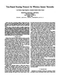
3. Network model and assumptions We make following assumptions for our sensor network: 1. Nodes are dispersed randomly following a Uniform distribution in a 2-dimensional space. 2. The energy of sensor nodes cannot be recharged. 3. Nodes are location unaware i.e. they are not equipped with any GPS device. 4. The nodes are capable of transmitting at variable power levels depending on the distance to the receiver as in [16]. For instance, the MICA Motes use MSP430 [17] series micro controller which can be programmed to 31 different power levels. 5. The nodes can estimate the approximate distance by the received signal strength, given the transmit power level is known, and the communication between nodes in not subject to multipath fading. The fifth assumption mainly deals with the definition of different power levels for intra-cluster and inter-cluster communications. In this way, the node energy consumption can be remarkably reduced so as to further prolong sensor network lifetime. In this paper, for simplicity, we assume the power level is continuous. In most local clustering algorithms in wireless sensor networks, to prolong the sensor network lifetime, the probability of a sensor node’s being selected as a cluster head primarily depends on its own residual energy. However, in some special cases, it doesn’t help balance the energy load for the proper nodes. As a result, it may cause the problem that some nodes will be exhausted quickly [5]. For instance, as shown in Figure 1, let us consider a sensor network composed by five nodes.

Figure 1. Cluster head election

First we select cluster head with amount of the residual energy of node, so in cluster range R1 node B elected as cluster head, because amount of the residual energy of node B is higher than that of the other nodes, because of the distance not considered it may the energy of node among sending data to cluster head energy of the node is remarkably reduced and die soon. If

38


we target only distance, therefore node C elected as a cluster head, considering the energy of node C is lower than other nodes and if selected as cluster head It may that energy’s terminated and dies, in among of sending data to the base station, so the network life time is reduced. In order to solve the problems mentioned above, we target, compositions of distance and residual energy for cluster head election. We present a novel energy and distance-aware routing protocol TBRP which can meet all the requirements listed previously. In the next section, we will describe the TBRP algorithm in details.

3.1. Proposed algorithm In TBRP protocol, each node stores the information about its neighbors, in a neighborhood table, as shown in table 1. At the beginning of each round, each node broadcasts the Ech_Msg, which contains residual energy’s, within radio range r. All nodes within the cluster range of one node as the neighbors of this node. Each node receives the Ech_Msg, from all neighbors in its cluster range and updates the neighborhood table and generates fuzzy number (FN). In our protocol for selecting the cluster head we use this formula: (1) The parameters and massage used in formula 1 and tree formation as shown in table2. Table 1. Parameters used in formula 1 Parameter

description

vi

Node i

vj

a neighbor node in cluster range of Vi

REv i

Residual energy of

Disv j

Distance between

REv j

Residual energy of

CHS

Cluster head selection

r

Intra communication radio range

vi vi ,v j vj

Ech_Msg

Elect cluster head massage

Crt_Msg

Create tree massage

For example, as shown in Figure 1, node A~E within the radio range (R1, R2). Now we attempt to determine the cluster heads. According figure 1 the nodes A, B, C within each other radio cluster head range and are neighborhood. And similarly, node C, D, E is neighborhood. In radio range R1 node D and within R2 node B elected as a cluster head. In order to reduce the energy consumption in each round, we assume that the plain nodes join the nearest head. We see that node C within two radio range (R1, R2) and if couldn’t elected as a cluster head it join to the nearest cluster head, so Node C join to the cluster head B. Table 2. Radio range R1 Node

Distance from neighbors

Residual Energy of

Residual Energy

39


A B C

neighbors 7,2 3,2 3,7

(B=6,C=2) 6,3 1,3

3 7 2

Table 3. Radio range R21 Node

Distance from neighbors

D E C

(E=5,C=3) 5,4 3,4

Residual Energy of neighbors 10,2 6,2 6,10

Residual Energy 6 10 2

In TBRP protocol, we have uniform energy consumption among all nodes, because the cluster heads always keep rotation in whole lifespan of network. By reduction of energy consumption for each round, the network lifetime is extended. Cluster formation pseudo code is shown below: for all nodes 1. Status ready 2. broadcast Node Residual_Msg to all neighbor nodes 3. receive Node_Residual_Msg from all neighbor nodes 4. compute distance from neighborhood 5. update neighborhood table 6. Node compute_FN() 7. if (FN >all neighborhood (FN)) 8. Status Head 9. else { 10. Status member 12. if (node existing in more than one cluster head range) 12. Node joins to closer cluster head} 13. endif Node compute_ FN () DN= ((Distance to Neighbor / 2 *100 ) and generate fuzzy number) Re= ((Residual energy /initial energy) and generate fuzzy number) n

Generate fuzzy election number ( FEN = ∑ X i ×A L i ) i =1

Return FN

4. Fuzzy routing tree In this section we use fuzzy decision criteria for constructing routing tree on cluster head nodes, that extremely save energy in cluster heads on the tree, and energy consumption is well-balanced among all sensor nodes. For selecting parent nodes in the tree, TBRP consider three parameter:

40


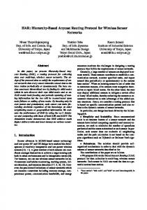
Amount of energy consumption in the cluster head. Amount of Residual energy in the cluster head. Distance between cluster head node and base station. Considering the application type, the number of this criteria and its eligibility are changeable by the base station. In TBRP, after clustering, Base station broadcast the Criteria message to the all cluster heads, which contains decision criteria and its values. After receiving this massage by the all cluster heads, each of them generate a fuzzy election number for it self. In the next state cluster heads broadcast within a radius R the Crt_Msg message, which contains node ID and fuzzy election number (FEN). The cluster head compares its own FEN and the FEN contained in the Crt_msg received from its neighbor cluster head. If it has smaller FEN, it selects the node that has the largest FEN as its parents and sends the CHILD message to notify the parent node. Finally, after a specified time, a fuzzy routing tree will be constructed; whose root node has the largest weight among all cluster heads in the same independent connected component. After routing tree construction, cluster heads broadcast a TDMA schedule to their active member nodes to be ready for data gathering. For example, assume that we have a network as shown in figure 2; nodes A to E are cluster heads. Our target is to construct a tree with efficient energy consumption on cluster heads. For this reason TBRP use fuzzy decision criteria to do this work, that saving energy in cluster heads and extend the network lifetime by balancing the energy load among all the nodes. As shown in figure 4, node B receives a Crt_Msg message containing FEN from A, C, D, E and select node A to be its parent. As the FEN of node A greater than FEN of node B, therefore node B select node A as it’s parent. Similarly, node D and C chooses B as their parent, while D chooses A as its parent. Node A receives a Crt_Msg message from nodes B and C, but their weight is less than node A, so A will be their parent and tree is constructed. In the tree structure we have one node to communicate directly with the base station, so A is root node in our fuzzy routing tree. The pseudo code for Fuzzy routing tree construction is shown in below. After clustering 1. Base Station Broadcast (criteria [], criteria value []) 2. FEN= Cluster head compute_ FEN () 3. Cluster head Broadcast (Crt_msg) 4. Cluster head receive Crt_msg 5. Cluster head Broadcast (myID, FEN) 6. Wait T1 7. ParentNode = Neighbor which send Max FEN 8. Send ( myID, CHILD) to ParentNode 9. IF isCluster Head 10. Broadcast TDMA schedule to active node

4.1. Fuzzy election number generation As described, in this paper we target three factors for election the cluster head. First we gather cluster head information (see table 3) and then generate X 1 , X 2 , X 3 criteria values (see table 4)using the pseudo code for Fuzzy election number generation as shown in Figure 2.

41


Figure 2. Fuzzy spanning routing tree formation

The pseudo fuzzy election number generation ----------------------------------------------------------------------------------Cluster head compute_ FEN () HEC= ((N/Cluster Number) and generate fuzzy number) DB= ((Distance to Base station / 2 *100 ) and generate fuzzy number) Re= ((Residual energy /initial energy) and generate fuzzy number) n

Generate fuzzy election number ( FEN = ∑ X i ×A L i ) i =1

Return FEN Table 4. Cluster information

CH

Cluster Number

Residual Energy

Distance to Base Station

A

5

2J

5m

B

8

2J

3m

C

6

1J

2m

D

3

1.5 J

6m

E

7

1.75 J

1.5 m

Table 5. FEN generated by all cluster heads

Criteria

-0.8 Energy consumption

A B

0.960 0.936

0.9 0.9

-0.9 Distance to Base Station 0.968 0.980

C D E

0.952 0.976 0.944

0.45 0.675 0.7875

0.987 0.961 0.990

Alternative

CH

42

0.9 Residual Energy

Fuzzy Election Number 2.828 2.816 2.389 2.612 2.7215


For example assume that we will compute FEN for a cluster head A, therefore we have: FEN 1 = AL1 ( X 1,1 ) + AL 2 ( X 1,2 ) + AL 3 ( X 1,3 ) And similarly other FEN j , so computed. In general for computing the FEN we define the formula 2: n

(2)

FEN jm=1 = ∑ X

j ,i

×ALi

i =1

Table 6. show the parameters used in formula 2 Parameter HEC DB Re FEN AL m

Xi n

ALi FEN

j

description Head Energy consumption Distance to Base station Residual energy fuzzy election number Alternative Number of cluster heads The ith element of decision criteria Number of decision criteria The ith element of alternative Fuzzy election number that generated by cluster head j‘``

4.2. Latency in TBRP LEACH uses direct communications from cluster heads to the BS. Therefore, with around 5% of nodes acting as cluster-heads in a 100-node network there are at least five long distance transmissions from five cluster-head nodes to BS. Time required to complete a single round can be estimated in the following way: if we consider that there are approximately 20 nodes per cluster for a 100-node network with 5% nodes acting as cluster-heads and if t unit of time is required for one node to transmit information to the cluster-head then with a TDMA schedule for 19 nodes requires approximately 19t unit of time to collect data from all the nodes in a cluster. After that with a CSMA MAC the last one among five cluster-heads may have to wait around 4t unit of time. In total 23t unit of time may require to before sending the last information from the network. This time requirement may vary due to the randomness of the network but we consider here the ideal case for the LEACH. Whereas in PEGASIS, each node transmits to the next and receives from its previous nearest neighbor except the end two nodes in a chain. Only one node is responsible to collect and transmit to the BS during each round. So long distance transmission reduces to bare minimum i. e. only one. If we assume it needs approximately same unit time delay t to transmit from one node to the next node, then for an N-node network, if the leader is the end node in the chain, other end needs (N-1) t unit of delay to reach the leader node. Therefore, for a 100-node network the delay yields 99t units.Considering our simulations, in worst case we have six cluster head , 20 member node

43


and three parent node on fuzzy routing tree for a 100-node network, Therefore extra (CN-1)t i.e. 19t of time required that member node to send data to the cluster head. As described, in fuzzy tree parent nodes (PN) collect the information from child’s and sends to the root parent,(Or root node), so (PN+1) t i.e. 4t unit of delay may occur that Cluster nodes on tree to send data to the base station. In total there may be (CN-1) t + (PN+1) t units i. e. 23t units of delay. Comparison between LEACH, PEGASIS and TBRP in one round of data transmission for a 100-node network, as shown in Table 7. Table 7. Comparison between LEACH, PEGASIS and TBRP Protocol LEACH TBRP PEGASIS

Delay 23 Unit 23 Unit 99 Unit

Table 8. Simulation parameters Parameters

Description

M*M

Simulation Area Number of Node Cluster radius R Sensing radius rs Sink position Initial energy Data packet size electronics energy free space coefficient

N R rs

Ps Ei Ldata Eelec efs

Value (0,0)~(100,100) 100~500 35 m 15 m At(50,200) 2J 200 Bytes 50 nJ/bit 10 nJ/bit/m2

5. Experiments and simulations result For theses experiments, a network of N sensor nodes in an 100? 00 m 2 area is considered. The N nodes are assumed to be uniformly distributed over the area, every simulation result shown below is the average of 100 independent experiments where each experiment uses a different randomly-generated. All parameters are given in Table 4. A simple radio model that also can be found in [16] has been adopted. Figure 3 shows the relationship between the number of cluster heads, the number of independent connected components, and network size. As the network size increases, it can be seen that the number of independent components is increasing too.

44


Number of cluster heads

Number of connected componnents

80 70 Value

60 50 40 30 20 10 500

400

300

200

100

0

Number of nodes

Figure 3. The number of heads and the number of connected components

HEED 750

TBRP

700 650 600

LEACH

550 500

Round

450 400 350 300 250 200 150 100 50 0 0

25

50

75

100

125

150

175

200

Base station position

Figure 4. Sink node position and network lifetime.

Figure 5 shows that the lifetime of the network between LEACH, HEED, and TBRP protocols vary with the number of nodes from 100 to 500. It is obvious that TBRP is uniformly better independent of node density. Well, this may due to the following reasons. First, alternating the role of CH can balance energy consumption among these clusters member. Second, our fuzzy spanning tree is effective in prolonging the lifetime of CHs. Third, our CH election algorithm more energy efficient, as a result extend the network lifetime.

45


Network lifetime based on Number of Rounds

HEED

TBRP

1800 1600 LEACH

1400 1200 1000 800 600 400

500

450

400

350

300

250

200

100

0

150

200

Number of Nodes

Figure 5. Network lifetime represented by number of rounds and sensor nodes

Figure 6 shows the total remaining energy of the network in three protocols for 20 rounds, with the number of node 100. It shows that TBRP balances the energy consumption among cluster heads best. HEED

TBRP

199

LEACH

Network Energy

197

195

193

191

189

187

185 1

2

3

4

5

6

7

8

9

10 11 12 13 14 15 16 17 18 19 20

Round

Figure 6. The total remaining energy of the network

The definitive improvement of TBRP from PEGASIS is that, the latency in data delivery is greatly minimized. Figure 7 shows that where, for 100 rounds, PEGASIS requires around 1800 seconds, TBRP requires only 200 of that time.

46


Time(Seconds)

3000

TBRP

PEGASIS

2000

1000

0 10

20

30

40

50

Number of Rounds

Figure 7. Time requirement for multi hop transmission data to the base station

8. Conclusion & future works In this paper, we propose a novel energy and distance-aware routing protocol for prolong the sensor network lifetime. TBRP clusters sensor nodes into groups and builds fuzzy routing tree among cluster heads for energy saving communication and minimizing latency in data delivery. Simulation result show that, when compared other schema TBRP outperforms significantly in optimizing cluster heads energy consumption, amount of data gathered, and Improving system lifetime. In future work we can use fuzzy decision criteria for intra cluster coverage problem and so, for electing optimum cluster head.

References [1]. Ming Liu, Jiannong Cao, Guihai Chen and Xiaomin Wang . 2009 An Energy-Aware Routing Protocol in Wireless Sensor Networks ,(Published Sensors 2009, 9), 445-462; doi:10.3390/s90100445 [2] W. Heinzelman, A. Chandrakasan, and H. Balakrishnan 2002 An Application-Specific Protocol Architecture for Wireless Microsensor Networks, IEEE Trans. Wireless Communication, vol. 1, no. 4, pp. 660-670, Oct. 2002 [3] O. Younis and S. Fahmy, “HEED: A Hybrid, Energy-Efficient, Distributed Clustering Approach for Ad Hoc Sensor Networks,” IEEE Trans. Mobile Computing, vol. 3, no. 4, pp. 660-669, Oct.-Dec. 2004. [4] S. Lindsey, C. Raghavendra, and K. M. Sivalingam, “Data Gathering Algorithms in Sensor Networks Using Energy Metrics,” IEEE Trans. Parallel and Distributed Systems, vol. 13, no. 9, pp. 924-935, Sep. 2002. [5] W. Heinzelman, A. Chandrakasan, and H. Balakrishnan, “Energy-Efficient Protocol for Wireless Microsensor Networks,” in Proc. 33rd Annu. Hawaii Int. Conf. System Sciences, Hawaii, 2000. [6] S. Lindsey and C. S. Raghavendra, “PEGASIS: Power Efficient Gathering in Sensor Information Systems,” in Proc. Aerospace Conf. Los Angeles, 2002. [7]. Lee, S.H.; Yoo, J.J.; Chung, T.C. Distance-based Energy Efficient Clustering for Wireless Sensor Networks. In Proceedings of the 29th Annual IEEE international Conference on Local Computer Networks (LCN’04), 2004 [8]. Mhatre, V.; Rosenberg, C. Homogeneous vs. Heterogeneous Clustered Networks: A Comparative Study. In Proceedings of IEEE ICC 2004, June 2004.

47


[10]. Xue, Q.; Ganz, A. Maximizing Sensor Network Lifetime: Analysis and Design Guides. In Proceedings of MILCOM, October 2004. [11]. Chan, H.; Perrig, A. ACE: An Emergent Algorithm for Highly Uniform Cluster Formation. In Proceedings of the First European Workshop on Sensor Networks (EWSN), 2004. [12]. Ye, M.; Li, C.F.; Chen, G.; Wu, J. EECS: An Energy Efficient Clustering Scheme in Wireless Sensor Networks. Int. J. Ad Hoc Sensor. Network. 2007, 3, 99-119. [13] D. Tian, and N. D. Georganas. A Node Scheduling Scheme for Energy Conservation in Large Wireless Sensor Networks. Thesis, Multimedia Communications Research Laboratory,School of Information Technology and Engineering, University of Ottawa, 2002. [14] J.M. McCune. Adaptability in sensor networks. Undergraduate Thesis in Computer Engineering, University of Virginia, April 2003. [15] I. Texas Instruments, "MSP430x13x, MSP430x14x Mixedm Signal Microcontroller. Datasheet, " 2001. [16] W. Heinzelman, A. Chandrakasan, and H. Balakrishnan, "An Application-Specific Protocol Architecture for," IEEE Transactions on Wireless Communications, vol. 1, 2002.

48