numerical computation of stress waves in solids

NUMERICAL COMPUTATION OF STRESS WAVES IN SOLIDS

Xiao LIN

Lehr-und Forschungsgebiet fur Mechanik RWTH Aachen University of Technology Aachen, Germany

To my parents: LIN Ying-Guang and CHEN Zhen :

Preface Propagation of stress waves in solids is governed by a system of hyperbolic partial dierential equations. Resolution of this system is always a challenge for scientists and engineers in terms of research and applications. An analytical solution is usually dicult to nd due to the inherent complication of the mathematical formulation. With modern computers, numerical solutions are possible even for complicated body geometry, material properties and various loading conditions. However, a numerical method must be available to achieve this goal. This book presents methods for numerical modeling of stress wave propagation in solids. It aims to solve two-dimensional problems which have direct applications in engineering. The nite dierence method is our main tool; of course, other methods, e.g., boundary element method, can be applied, too, for linear elastic problems. But we will concentrate on nite dierence method. I hope that this book serves as a reference book not only for scientists and engineers but also for students and graduate students at universities who study mathematical physics and solid dynamics. The book is the result of my recent research in computational solid mechanics. I became interested in stress wave problems in 1981 when I was studying at the East China Institute of Technology, Nanjing. I wondered if an elegant technique like the method of characteristics for one-dimensional solids could be found to deal with two-dimensional problems. I must thank my doctorate supervisor Professor WEI Hui-Zhi who gave me a wide range of knowledge in applied mathematics and mechanics, providing me with an excellent background for my later research work. After nishing my Ph.D., I obtained a research fellowship from the Alexander von Humboldt Foundation from 1989 to 1991, for research with Professor Josef Ballmann at the RWTH Aachen University of Technology, Germany. I thank the AvH Foundation for this opportunity which has brought my dream into a reality. I then began research on stress wave propagation in two-dimensional solids using nite dierence methods. With the help of Professor Ballmann, this research continued from 1991 till the present moment. It is also supported by the Deutsche Forschungsgemeinschaft (DFG) under Grant No. Ba 661/12-1.

6

Preface

I give my heartfelt thanks to Professor Ballmann who has not only provided with me the best working conditions I could hope for, but many opportunities for taking part in international conferences and visiting many universities that I could obtain up-to-date materials in this research eld. He is the leader of many research projects on stress waves which have been undertaken in our institute | Lehr-und Forschungsgebiet fur Mechanik | since 1979 with the support of DFG. As my supervisor, he has transmitted many ideas and experiences of his own and his former students to me. In this sense, this book is a research summation of this institute, too. From 1995 I have been invited by Professor J. Glimm to join his research group at the University at Stony Brook, to perform numerical modeling on high strain-rate deformation of hyperelastic-viscoplastic materials. With this opportunity I have constructed a solid modeling library as an extension of the Stony Brook front tracking code. Section 6.6 represents the outcome of my research at Stony Brook with Prof. Glimm, Prof. B. Plohr, Prof. J. Grove, Dr. D. Sharp at Los Alamos National Laboratory, and Dr. J. Walter at the Army Research Laboratory. The funding support from the U.S. Army Research Oce under Grant DAAL-04-94-9510414 is also greatfully acknowledged. Especially, I would like to thank Prof. J. Glimm who has read this book as a whole and given me many valuable comments as well as improvements in the English usage. I would like, too, to thank Prof. R. Jeltsch at ETH Zurich University of Technology, Prof. J. Engelbrecht of Estonian Academy of Sciences, Prof. T.C.T. Ting at University of Illinois at Chicago, Prof. L.M. Brock at University of Kentucky, Prof. A.J. Rosakis at California Institute of Technology, Prof. Y.M. Chen at SUNY at Stony Brook, Prof. J.J. Xu at McGill University, for their useful comments on this book before publishing. I would also like to thank my colleagues Dr. K.-S. Kim, Dr. C.A. Muller, Dr. I. Grotowsky, Dr. R.J. Niethammer, Dr. A. Rivinius, Dr. U. Sprecht, Dr. Y.-G. Zhang, and my assistants Mr. T. Richard, Mr. C. Budorovits and Mr. I. Mikulic, and all others studying and working in our institute for providing me with a harmonious atmosphere during daily research work, and for their help to me in countless other ways. Finally, I would like to thank my wife LI Xue-Qun, our daughters Jie-Liang and Wendy who enthusiastically supported my writing of this book. Xue-Qun took over all household duties and they endured many lonely weekends and holidays without me, allowing me not only much more time but also more energy to do the research. Stony Brook, June 1996

Xiao LIN

Contents Preface

5

1 Introduction

13

2 Schemes for One-Dimensional Solids

20

1.1 Why this book was written : : : : : : : : : : : : : : : : : : : : : : : : : 1.2 How this book was written : : : : : : : : : : : : : : : : : : : : : : : : : 1.3 References : : : : : : : : : : : : : : : : : : : : : : : : : : : : : : : : : : 2.1 Introduction : : : : : : : : : : : : : : : : : : : : : 2.2 Lax-Wendro method for rods : : : : : : : : : : : 2.2.1 Governing equations : : : : : : : : : : : : 2.2.2 Lax-Wendro scheme : : : : : : : : : : : : 2.2.3 Von Neumann condition and CFL number 2.2.4 Elastic-plastic problems : : : : : : : : : : 2.3 Godunov's method for rods : : : : : : : : : : : : 2.3.1 Simple wave solution : : : : : : : : : : : : 2.3.2 Riemann solver and Godunov's method : : 2.3.3 The second-order Godunov scheme : : : : 2.3.4 A test example : : : : : : : : : : : : : : : 2.3.5 A computer program : : : : : : : : : : : : 2.4 Combined stress waves in a thin-walled tube : : : 2.4.1 Governing equations : : : : : : : : : : : : 2.4.2 Characteristic relations : : : : : : : : : : : 2.4.3 Loading path in stress space : : : : : : : : 2.5 Numerical modeling of combined stress waves : : 2.5.1 Riemann problems : : : : : : : : : : : : : 2.5.2 Three basic loading paths : : : : : : : : : 2.5.3 Loading paths for general cases : : : : : :

: : : : : : : : : : : : : : : : : : : :

: : : : : : : : : : : : : : : : : : : :

: : : : : : : : : : : : : : : : : : : :

: : : : : : : : : : : : : : : : : : : :

: : : : : : : : : : : : : : : : : : : :

: : : : : : : : : : : : : : : : : : : :

: : : : : : : : : : : : : : : : : : : :

: : : : : : : : : : : : : : : : : : : :

: : : : : : : : : : : : : : : : : : : :

: : : : : : : : : : : : : : : : : : : :

: : : : : : : : : : : : : : : : : : : :

: : : : : : : : : : : : : : : : : : : :

13 16 18

20 21 21 22 24 27 28 28 29 31 33 35 39 39 42 43 45 45 48 50

8

Contents

2.5.4 The second-order Godunov method : : : : : : 2.5.5 Numerical examples : : : : : : : : : : : : : : 2.6 One-dimensional TVD method : : : : : : : : : : : : : 2.6.1 The concept of TVD : : : : : : : : : : : : : : 2.6.2 CFL number and wave parameter : : : : : : : 2.6.3 The TVD scheme for a simple wave : : : : : : 2.6.4 The TVD method for a complex wave system 2.6.5 Two examples : : : : : : : : : : : : : : : : : : 2.7 References : : : : : : : : : : : : : : : : : : : : : : : :

3 A Scheme for Two-Dimensional Solids

: : : : : : : : :

: : : : : : : : :

: : : : : : : : :

: : : : : : : : :

3.1 Introduction : : : : : : : : : : : : : : : : : : : : : : : : : : : 3.2 The anti-plane shear problem : : : : : : : : : : : : : : : : : 3.2.1 Governing PDEs for a solid under anti-plane shear : 3.2.2 Some basic aspects of numerical modeling : : : : : : 3.2.3 Plastic loading paths in a stress space : : : : : : : : : 3.2.4 Flux calculations : : : : : : : : : : : : : : : : : : : : 3.2.5 Updating of the functions : : : : : : : : : : : : : : : 3.2.6 Treatment of boundary conditions : : : : : : : : : : : 3.2.7 Dynamic stress intensity factors : : : : : : : : : : : : 3.2.8 A semi-in nite crack subjected to a step pulse : : : : 3.2.9 A nite crack subjected to a Heaviside pulse : : : : : 3.2.10 A computer program : : : : : : : : : : : : : : : : : : 3.3 Zwas' method for linear plane problems : : : : : : : : : : : : 3.3.1 Governing equations : : : : : : : : : : : : : : : : : : 3.3.2 Treatment of boundary conditions : : : : : : : : : : : 3.3.3 Semi-in nite plane subjected to an impact : : : : : : 3.3.4 Stress intensity factor in an in nite body with crack : 3.3.5 Chen's problem : : : : : : : : : : : : : : : : : : : : : 3.4 Plane strain problems : : : : : : : : : : : : : : : : : : : : : : 3.4.1 Elastic-plastic loading path : : : : : : : : : : : : : : 3.4.2 Governing equations : : : : : : : : : : : : : : : : : : 3.4.3 Flux calculations : : : : : : : : : : : : : : : : : : : : 3.4.4 Boundary conditions : : : : : : : : : : : : : : : : : : 3.4.5 Updating the functions : : : : : : : : : : : : : : : : : 3.4.6 One-dimensional simple wave : : : : : : : : : : : : :

: : : : : : : : : : : : : : : : : : : : : : : : : : : : : : : : : :

: : : : : : : : : : : : : : : : : : : : : : : : : : : : : : : : : :

: : : : : : : : : : : : : : : : : : : : : : : : : : : : : : : : : :

: : : : : : : : : : : : : : : : : : : : : : : : : : : : : : : : : :

: : : : : : : : : : : : : : : : : : : : : : : : : : : : : : : : : :

: : : : : : : : : : : : : : : : : : : : : : : : : : : : : : : : : :

52 53 57 57 58 61 63 64 66

68

68 69 69 70 74 76 78 79 81 83 83 85 94 94 95 97 97 100 103 103 105 106 108 109 109

Contents

3.4.7 Semi-in nite crack subjected to a Heaviside pulse wave 3.4.8 A nite crack subjected to a shock wave : : : : : : : : 3.5 A brief examination of plane stress problems : : : : : : : : : : 3.5.1 Basic governing equations : : : : : : : : : : : : : : : : 3.5.2 CFL number : : : : : : : : : : : : : : : : : : : : : : : 3.5.3 A result for unloading and reyielding phenomena : : : 3.6 References : : : : : : : : : : : : : : : : : : : : : : : : : : : : :

4 The Method of Bicharacteristics

9

: : : : : : :

: : : : : : :

: : : : : : :

: : : : : : :

: : : : : : :

4.1 Introduction : : : : : : : : : : : : : : : : : : : : : : : : : : : : : : : : : 4.2 Second-order bicharacteristic schemes : : : : : : : : : : : : : : : : : : : 4.2.1 Basic equations and bicharacteristic relations : : : : : : : : : : : 4.2.2 General expressions for second-order accurate bicharacteristic solutions : : : : : : : : : : : : : : : : : : : : : : : : : : : : : : : : 4.2.3 The Lax-Wendro scheme : : : : : : : : : : : : : : : : : : : : : 4.2.4 Methods to get a higher CFL number : : : : : : : : : : : : : : : 4.2.5 The least squares technique and weighting functions : : : : : : : 4.2.6 Some comments on the bicharacteristic schemes : : : : : : : : : 4.2.7 Application to crack initiation and growth : : : : : : : : : : : : 4.3 Total variation diminishing schemes : : : : : : : : : : : : : : : : : : : : 4.3.1 Two-dimensional Riemann problems : : : : : : : : : : : : : : : 4.3.2 A rst-order accurate bicharacteristic solution : : : : : : : : : : 4.3.3 Godunov's scheme for two dimensions : : : : : : : : : : : : : : : 4.3.4 The hybrid method : : : : : : : : : : : : : : : : : : : : : : : : : 4.3.5 A complete solution to the 2-D Riemann problem : : : : : : : : 4.3.6 The TVD scheme : : : : : : : : : : : : : : : : : : : : : : : : : : 4.3.7 A test: the half plane subjected to shear impact : : : : : : : : : 4.4 An application to anti-plane shear : : : : : : : : : : : : : : : : : : : : : 4.4.1 The governing equations : : : : : : : : : : : : : : : : : : : : : : 4.4.2 The two-dimensional Riemann solution : : : : : : : : : : : : : : 4.4.3 One-dimensional simple wave : : : : : : : : : : : : : : : : : : : 4.4.4 A nite crack subjected to a quasi-static loading : : : : : : : : : 4.4.5 A further examination of elastic-plastic problems : : : : : : : : 4.5 Three-dimensional schemes : : : : : : : : : : : : : : : : : : : : : : : : : 4.5.1 The governing equations : : : : : : : : : : : : : : : : : : : : : : 4.5.2 The second-order scheme : : : : : : : : : : : : : : : : : : : : : :

111 113 115 115 117 118 120

123 123 124 124

126 128 131 132 135 138 143 143 145 147 148 150 152 154 155 155 158 161 162 163 164 164 165

10

Contents

4.5.3 The rst-order scheme and the TVD scheme : : : : : : : : : : : 169 4.6 References : : : : : : : : : : : : : : : : : : : : : : : : : : : : : : : : : : 169

5 Axisymmetric Elastic Waves

5.1 Introduction : : : : : : : : : : : : : : : : : : : : : : : : : : : : : : 5.2 Scheme for a regular mesh : : : : : : : : : : : : : : : : : : : : : : 5.2.1 System of PDEs for axisymmetric elastic waves : : : : : : 5.2.2 Numerical scheme : : : : : : : : : : : : : : : : : : : : : : : 5.2.3 First-order scheme and hybrid method : : : : : : : : : : : 5.2.4 A half-space problem : : : : : : : : : : : : : : : : : : : : : 5.2.5 A penny-shaped crack : : : : : : : : : : : : : : : : : : : : 5.2.6 The initial wave pattern in an impacted circular rod : : : : 5.3 Two-grid method : : : : : : : : : : : : : : : : : : : : : : : : : : : 5.3.1 Problem of a cylindrical bar with a spherical end : : : : : 5.3.2 Governing PDEs in spherical coordinates and computation 5.3.3 Numerical results of wave focusing : : : : : : : : : : : : : 5.4 Curvilinear grids and related schemes : : : : : : : : : : : : : : : : 5.4.1 Formulation of the curvilinear grid problem : : : : : : : : 5.4.2 Curvilinear grid generation : : : : : : : : : : : : : : : : : : 5.4.3 A special technique for a grid near a boundary : : : : : : : 5.4.4 Example { a domain with an ellipse : : : : : : : : : : : : : 5.4.5 The dierence scheme for an irregular grid : : : : : : : : : 5.4.6 The treatment of boundary conditions : : : : : : : : : : : 5.4.7 Example { stress wave focusing : : : : : : : : : : : : : : : 5.5 References : : : : : : : : : : : : : : : : : : : : : : : : : : : : : : :

6 Stress Waves in Other Materials

6.1 Introduction : : : : : : : : : : : : : : : : : : : : : : : : : : : : 6.2 Anisotropic stress waves : : : : : : : : : : : : : : : : : : : : : 6.2.1 Linearly elastic waves in a cubic material : : : : : : : : 6.2.2 Constitutive formulation of cubic materials : : : : : : : 6.2.3 The plane strain problem : : : : : : : : : : : : : : : : : 6.2.4 The formation of a plastic zone at a crack tip : : : : : 6.2.5 Elastic waves in an orthotropic material : : : : : : : : 6.2.6 Elastic-plastic waves in transversely isotropic materials 6.3 Viscoelastic and elastic-viscoplastic waves : : : : : : : : : : :

: : : : : : : : :

: : : : : : : : :

: : : : : : : : : : : : : : : : : : : : : : : : : : : : : :

: : : : : : : : : : : : : : : : : : : : : : : : : : : : : :

: : : : : : : : : : : : : : : : : : : : : : : : : : : : : :

172 172 173 173 174 175 176 177 180 183 183 185 186 188 188 189 191 192 194 196 201 201

204 204 205 205 210 212 215 217 218 219

Contents

6.4

6.5

6.6

6.7

11

6.3.1 The type of linearly viscoelastic system : : : : : : : : : 6.3.2 Visco-eects on numerical computations : : : : : : : : 6.3.3 Stress waves in Maxwell's viscoelastic body : : : : : : : 6.3.4 Elastic-viscoplastic stress waves : : : : : : : : : : : : : Phase transition wave : : : : : : : : : : : : : : : : : : : : : : : 6.4.1 Stress-induced phase transition in materials : : : : : : 6.4.2 The numerical scheme for phase transition waves : : : 6.4.3 Phase transition under plane strain : : : : : : : : : : : 6.4.4 Phase transition under plane stress : : : : : : : : : : : Hydro-elastic-plastic waves : : : : : : : : : : : : : : : : : : : : 6.5.1 Hydro-elastic-plastic materials : : : : : : : : : : : : : : 6.5.2 Riemann problem : : : : : : : : : : : : : : : : : : : : : 6.5.3 Elastic-plastic eects : : : : : : : : : : : : : : : : : : : 6.5.4 Numerical scheme { ux calculation : : : : : : : : : : : 6.5.5 Numerical scheme { CFL number and mesh movement 6.5.6 Numerical scheme { updating of functions : : : : : : : 6.5.7 Example { Taylor's pressure bar : : : : : : : : : : : : : Stress waves in hyperelastic-plastic materials : : : : : : : : : : 6.6.1 The PDEs for hyperelastic material : : : : : : : : : : : 6.6.2 The equation of state for hyperelastic material : : : : : 6.6.3 The hyperelastic-viscoplastic material : : : : : : : : : : 6.6.4 The bicharacteristic analysis : : : : : : : : : : : : : : : 6.6.5 Standard nite dierence scheme : : : : : : : : : : : : 6.6.6 A review of Riemann problems : : : : : : : : : : : : : 6.6.7 An approximate two-dimensional Riemann solver : : : 6.6.8 Example for two-dimensional Godunov's method : : : : 6.6.9 The Riemann problem for material interfaces : : : : : : 6.6.10 Front tracking for material interfaces : : : : : : : : : : 6.6.11 Application to impact and penetration problems : : : : 6.6.12 A remark to the formulation of governing PDEs : : : : References : : : : : : : : : : : : : : : : : : : : : : : : : : : : :

7 The Covering Domain Method

: : : : : : : : : : : : : : : : : : : : : : : : : : : : : : :

: : : : : : : : : : : : : : : : : : : : : : : : : : : : : : :

: : : : : : : : : : : : : : : : : : : : : : : : : : : : : : :

: : : : : : : : : : : : : : : : : : : : : : : : : : : : : : :

: : : : : : : : : : : : : : : : : : : : : : : : : : : : : : :

219 220 222 225 227 227 228 230 233 236 236 238 241 242 245 246 249 250 250 251 257 259 261 262 264 267 268 271 273 275 276

279

7.1 Introduction : : : : : : : : : : : : : : : : : : : : : : : : : : : : : : : : : 279 7.2 The general formulation of CDM : : : : : : : : : : : : : : : : : : : : : 281 7.2.1 The superposition approach : : : : : : : : : : : : : : : : : : : : 281

12

Contents

7.3

7.4

7.5 7.6

Index

7.2.2 Coordinate transformation : : : : : : : 7.2.3 The basic problem : : : : : : : : : : : 7.2.4 Laplace and Fourier transforms : : : : Anti-plane shear stress waves : : : : : : : : : 7.3.1 The basic solution : : : : : : : : : : : 7.3.2 A test in a rectangular domain : : : : 7.3.3 Wave focusing in a circular domain : : In-plane stress waves : : : : : : : : : : : : : : 7.4.1 The governing equations : : : : : : : : 7.4.2 Basic solution for a semi-in nite plane 7.4.3 Some special techniques : : : : : : : : 7.4.4 The results of basic problems : : : : : 7.4.5 Two test problems : : : : : : : : : : : Remarks : : : : : : : : : : : : : : : : : : : : : References : : : : : : : : : : : : : : : : : : : :

: : : : : : : : : : : : : : :

: : : : : : : : : : : : : : :

: : : : : : : : : : : : : : :

: : : : : : : : : : : : : : :

: : : : : : : : : : : : : : :

: : : : : : : : : : : : : : :

: : : : : : : : : : : : : : :

: : : : : : : : : : : : : : :

: : : : : : : : : : : : : : :

: : : : : : : : : : : : : : :

: : : : : : : : : : : : : : :

: : : : : : : : : : : : : : :

: : : : : : : : : : : : : : :

: : : : : : : : : : : : : : :

283 285 286 288 288 292 294 295 295 296 301 303 303 308 310

312

Chapter 1 Introduction 1.1 Why this book was written Stress wave propagation in solids, which can be caused by impact or other impulsive loading, is a basic phenomenon encountered in many branches of physical sciences and engineering. The mathematical formulation of a stress wave is given by a system of hyperbolic partial dierential equations. The understanding of the wave problem is usually expressed as a solution to this system under given initial and boundary conditions. The research on stress waves began in the 1820's when Cauchy and Poisson [1.1] had developed governing PDEs for wave motion. For a long time people primarily were concerned with the characteristic wave speeds (or frequency) of PDEs. E.g., Poisson discovered in 1831 that two kinds of stress waves, i.e. the longitudinal wave and the transverse wave, can propagate in an elastic body; Rayleigh [1.2] proved in 1887 the existence of a surface wave; and Clifton [1.3] and Ting [1.4] found fast and slow plastic waves in a thin-walled tube. This research is most essential to obtain the solution for wave propagation in solids. Another important task is to search for the solution for the PDEs under given initial and boundary conditions. Physically, the stress components are of certain magnitudes which change during wave propagation. It is the change of stress intensity that causes changes in certain material properties, e.g. plasticity, viscosity, etc. In engineering design, the information of the distributions of stress, strain, and particle velocity in a structure is also important. In such cases, the system of PDEs must be solved for a solution. The solution methods can be mainly classi ed into two groups: analytical and numerical.

14

Chapter 1 Introduction

Due to diculties in mathematics, an analytical method is usually restricted to problems of simple geometry, simple material properties or simple loading conditions. One of the most important approaches is the method of characteristics in obtaining a solution for one-dimensional impact of elastic-plastic rods. It was developed by Taylor [1.5], von Karman [1.6] and Rahmatulin [1.7] during the World War II. If a simple wave region in the (x; t) plane exists, this method can give an exact solution. For a complex wave region, the method can also be applied in order to integrate the compatibility relations along characteristic lines. Other important approaches are the Laplace and Fourier transform methods in solving one- and two-dimensional linear elastic problems. The Cagniard-de Hoop method [1.8] is very signi cant since it allows the inverse Laplace transform to give an analytical solution. Numerical research for stress wave propagation has been in uenced by developments in computational uid dynamics. Since this system is hyperbolic, the methods for supersonic or unsteady inviscid ows in gas dynamics can be applied. One of the most successful applications is given to the one-dimensional impact of an elastic-plastic rod, where the method of characteristics can be applied directly. Because wave propagation can be clearly interpreted by characteristic lines in the (x; t) plane, the numerical solutions of this method are seen as analytical ones. For the two-dimensional propagation of stress waves in isotropic linear elastic bodies, Clifton [1.9] has transferred the method of bicharacteristics of Butler [1.10] in the unsteady ow of gas dynamics to linear elastodynamics, and contributed a dierence scheme. This scheme has the same stability condition as that of the Lax-Wendro scheme [1.11], i.e., a Courant-Friedrichs-Lewy (CFL) number less than 1 is required. A technique of reconstructing the values at the initial plane was used by Ballmann et al [1.12] in which the CFL number can be set to the limit 1. This technique has been generalized by Lin and Ballmann [1.13]. There is an increasing demand for numerical computation of stress waves in science and technology. In order to determine material properties, the stress wave interaction with a crack tip must be investigated in the eld of fracture mechanics. Only the numerical method can be used as a tool for studying this problem, where there are complicated body geometries, dierent material properties (plasticity, viscosity, composite etc.), and various loading conditions. In mechanical engineering, stress wave interactions between impacted machine elements must be calculated for power analysis. Instead of the simple model, e.g. one-dimensional rods, it is necessary to consider problems using the geometry of two-dimensional axisymmetry or even three-dimensional objects. There are also many other problems which arise in earthquake engineering and structural dynamics, in explosive prospecting and crack detection techniques which can be considered as

1.1 Why this book was written

15

stress wave propagation problems and which require numerical modeling. It is then an open question how to model stress wave propagation correctly. The rapid development of powerful software which uses the nite element method has brought convenience to structure analysis under static or quasi-static loading conditions. However, it has produced a negative eect on the research of stress waves. It seems sometimes that any problem of stress wave propagation induced by an impact can be modeled by modern software. As a matter of fact, stress waves governed by a hyperbolic system require special schemes, special time steps and mesh sizes in numerical modeling. To ignore these points would lead to inaccurate results. From a physical point of view, it is also unacceptable to simply transfer the computational technique from gas dynamics to solid dynamics even though both systems are hyperbolic. Solid mechanics has special characteristics of its own. In solids, singular points usually exist, e.g. the crack tip. The stress distribution near the singular point is very important and must be modeled as accurately as possible. In an elastic-plastic solid, there are four characteristic waves, i.e., the elastic longitudinal wave, the elastic transverse wave, the plastic fast wave, and the plastic slow wave. These waves may appear all together or in part. A solid region with plastic yield can undergo elastic unloading and later again a plastic reyielding, in which case the governing equations are dierent. If the dierent material properties are taken into account, the wave system also behaves dierently. It is the purpose of this book to summarize the achievements in numerical modeling of stress wave propagation in solids, especially in two dimensions, in order to meet the needs of today's science and technology. Fundamentally, the system is hyperbolic and thus, characteristic-based numerical schemes need to be developed for its numerical solution. Any good numerical scheme in gas dynamics, e.g. the Zwas scheme [1.14] may be adopted. It can also be seen that some new schemes, like the nite dierence scheme for systems with a source term, have been discovered in the research of solid dynamics [1.15, 1.16]. These are no doubt applicable to both solids and uids. Secondly, it is most important to concentrate on stress wave propagation in solids. As will be seen, a good scheme in gas dynamics may be a bad one when applied to solids. A solid can behave with dierent material properties, i.e. elastic, elastic-plastic, anisotropic, viscoplastic and so on. It is dicult to nd a scheme suitable for all materials. Each material needs a special formulation in computation. With this background, it is possible to apply all the basic understanding of characteristic analysis for wave speeds and existing exact solutions to con rm the accuracy of a numerical scheme and its results, which then can be usefully used in application.

16


1.2 How this book was written This book was written attempting to combine the mathematical formulation and the physical interpretation for each wave problem. In terms of computation, the governing equations, the methods and schemes will be dealt with in detail. The most important fundamental theories and many new developments of numerical schemes for hyperbolic PDEs in recent twenty years are included. In order to obtain numerical solutions for the stress wave propagation, we provide not only techniques for writing computer programs for two-dimensional problems but also ideas for the stability analysis. At the same time, the background of each problem in mechanics will be stated as clearly as possible, using the language of physics or practical applications. The exact solution is always used to compare with the numerical solution whenever possible, which will help us to understand the intrinsic quality of the numerical method. The results are always shown using clear diagrams, which can give direct physical explanations for stress wave propagation. Another feature of this book is that each subject is written as completely as possible, so as to limit the basic knowledge and references needed in order to read the book. This is better, not only for beginners, but also for those being familiar with numerical schemes but who lack understanding of solid mechanics, or for those who have been trained as mechanical engineers but need more mathematical knowledge. Although many mathematical techniques are used, the reader can also learn them while reading the book. Usually each problem is formulated using a system of hyperbolic PDEs. Physical language, such as anti-plane shear or plane strain is used to identify the system so that engineers can understand them at once. Then the numerical scheme is presented. Finally the solution obtained by the scheme is plotted in a graph with some physical explanations. We hope this procedure will be welcome by both mathematicians and engineers. The book is focused on the nite dierence method (from Chapter 2 to 6) and the boundary element method (Chapter 7) as tools for solving systems of hyperbolic PDEs arising in solid dynamics. The subjects and problems included in the book are taken from recent publications. Outlining elementary work, the book begins in Chapter 2 with the one-dimensional problem. Stress waves in a rod is examined in order to introduce basic knowledge, including the Lax-Wendro scheme, Riemann problems and Godunov's method as well as the CFL stability condition. Then a combined longitudinal and torsional wave in a thin-walled tube is used as a model to present the basic concept of a loading path

1.2 How this book was written

17

in stress space; this is also an important example for the distinction with the problems in gas dynamics. The last section introduces the modern TVD method. This chapter is easy to read even for the beginner who does not have any idea of numerical computations or stress waves at all. Of course, there are many great achievements of one-dimensional schemes. However, only a most important part, which can be applied to multi-dimensional problems in the followed chapters, will be presented. Chapter 3 examines the numerical modeling of stress wave propagation in a twodimensional elastic-plastic solid. A method extended from the Zwas scheme is applied throughout this chapter. The problem is discussed from the easy anti-plane shear to the dicult plane strain and plane stress, and from the simple linear elastic material to the complicated elastic-plastic material. The schemes for boundary conditions are also discussed so that the practical problem can be solved. Many numerical examples are presented in this chapter in order to provide readers with more information on the background of waves in solids. In Chapter 4 more techniques for constructing two-dimensional numerical schemes are presented by methods of bicharacteristics. First, one will read a second-order bicharacteristic scheme which includes the Zwas scheme as a special case. An approach is dealt with for the stability conditions of a dierence scheme. The feature of a scheme which models a singular point is also given. Then, a rst-order accurate scheme can be obtained by solving a two-dimensional Riemann problem. Based on these results, a hybrid method, or a TVD scheme can be constructed and applied to solve a problem like the shear impact in which the CFL number for the shock wave front is less than one. Afterwards, the bicharacteristic scheme is applied to an anti-plane shear problem for computation. A brief discussion of three-dimensional numerical schemes is given. Stress wave propagation in a two-dimensional axisymmetrical body is discussed in Chapter 5. Mathematically, the system of governing equations contains a source term. Instead of using the time-splitting technique, the numerical scheme combines the source term into the two steps of ux computation and function updating. Examples are presented only for a linear elastic material with wave focusing phenomena, but it is not dicult to extend the method to elastic-plastic materials. A two-grid technique for computation is presented. Finally, the formulation of a curvilinear grid and the related scheme is shown, which is useful in application. There are many kinds of solid materials whose properties can be represented by dierent constitutive relations. Stress wave propagation in those materials behaves dierently. Such problems are interesting in material science. The nite dierence scheme for ve kinds of materials are discussed in Chapter 6, i.e. anisotropic com-

18


posite material, viscoelastic or elastic-viscoplastic material, phase transition material, hydro-elastic-plastic material, and hyperelastic-viscoplastic material. The work mainly focuses on the mathematical formulation of the system in order to undertake numerical computation. The stress wave features of dierent materials are also represented by examples to show the physical backgrounds. The last chapter presents a covering domain method which belongs to a boundary element approach in modeling stress wave propagation in linear elastic solids. Instead of using Betti's reciprocal theorem of work, the boundary integral equations of elastodynamics are formulated by the principle of superposition which can give a direct physical explanation to the wave propagation. The anti-plane shear problem is rst solved and then the plane strain (or plane stress) problem. Basic solutions for both are obtained using Laplace and Fourier transforms, which have been presented in detail since they cannot be found in other references. The superposition procedure by numerics is most important in getting to a solution. We hope, this book will become a useful reference book for theoretical research, since many up-to-date numerical methods for modeling stress waves have been included; and this book will also be useful in engineering, because most subjects are characteristically two-dimensional and so have direct applications. This book, as previously stated, is also written for students who wish to study the numerical methods for systems of hyperbolic PDEs. From the experience of the author and his colleagues as well as his students, the quickest way to learn numerical computation is to read some computer programs. Therefore, two computer programs written in FORTRAN language, one for a one-dimensional rod problem and the other for a two-dimensional anti-plane shear problem, are included in this book.

1.3 References [1.1] A.E.H. Love, A Treatise on the Mathematical Theory of Elasticity, 4th edition, 287-292, Dover Publications, New York 1944. [1.2] L. Rayleigh, On waves propagated along the plane surface of an elastic solid, Proc. London Math. Soc. 17 (1887) 4. [1.3] R. J. Clifton, An analysis of combined longitudinal and torsional plastic waves in a thin-walled tube, Proceedings of the Fifth U.S. National Congress of Applied Mechanics, 465-480, University of Minnesota 1966. [1.4] T.C.T. Ting and Ning Nan, Plane waves due to combined compressive and shear stresses in a half space, Journal of Applied Mechanics 36 (1969), 189-197.

1.3 References

19

[1.5] G.I. Taylor, Propagation of earth waves from an explosion, British Ocial Report RC. 70 (1940); In: G.K. Batchelor (ed.), The Scienti c Papers of G.I. Taylor, Vol. 1, Mechanics of Solids, 456-, Cambridge University Press, Cambridge 1958. [1.6] T. von Karman, On the propagation of plastic deformation in solids, NDRC Report A-29, PB. 20276 (1942). [1.7] X.A. Rahmatulin, About spreading of unloading wave (in Russian), Appl. Mat. Mech. 9 (1945), 91. [1.8] J.D. Achenbach, Wave Propagation in Elastic Solids, North-Holland Publishing Company, Amsterdam 1973. [1.9] R.J. Clifton, A dierence method for plane problems in dynamic elasticity, Quarterly of Applied Mathematics 25 (1967), 97-116. [1.10] D.S. Butler, The numerical solution of hyperbolic systems of partial dierential equations in three independent variables, Proc. Roy. Soc. London A 255 (1960), 232-252. [1.11] P.D. Lax and B. Wendro, Dierence schemes for hyperbolic equations with high order of accuracy, Comm. Pure Appl. Math. 17 (1964), 381-398. [1.12] J. Ballmann, H.J. Raatschen and M. Staat, High stress intensities in focussing zones of waves; In: P. Ladeveze (ed.), Local eects in the analysis of structures, 235-252, Elsevier Science Publishers, Amsterdam 1985. [1.13] X. Lin and J. Ballmann, Improved bicharacteristic schemes for two-dimensional elastodynamic equations, Quarterly of Applied Mathematics 53 (1995), 383-398. [1.14] B. Eilon, D. Gottlieb and G. Zwas, Numerical stabilizers and computing time for secondorder accurate schemes, Journal of computational Physics 9 (1972), 387-397. [1.15] F. Wang, J.G. Glimm, J.W. Grove, B.J. Plohr and D.H. Sharp, A conservative Eulerian numerical scheme for elastoplasticity and application to plate impact problems, Impact of Computing in Science and Engineering 5 (1993), 285-308. [1.16] X. Lin and J. Ballmann, A numerical scheme for axisymmetric elastic waves in solids, Wave Motion 21 (1995), 115-126.

Chapter 2 Schemes for One-Dimensional Solids 2.1 Introduction This book deals with stress wave propagation in elastic-plastic solids which are governed by a hyperbolic system of partial dierential equations. For solutions in one space variable and time the problems can be solved analytically or numerically using the method of characteristics. However, many diculties arise when two- or three-independent space variables are taken into account. Other numerical methods are needed in order to study more complicated problems. Many nite dierence schemes have been developed in gas dynamics to model multidimensional unsteady ows. It is possible to apply these schemes to model the propagation of elastic-plastic waves in solids. But the solid material is dierent in several respects from a uid. For example, there may exist in one solid a plastic loading region and an elastic unloading region, whose governing equations are dierent and whose boundary is unknown in advance. To model such phenomena, the methods used in gas dynamics are generally not applicable. Some special techniques are needed. Stress waves propagate in solids along continuous characteristic lines or surfaces in the space-time domain. In a nite dierence method, however, the continuous body is divided into nite cells, and the functions are represented by a nite number of values in the cells. Therefore, it is particularly important for a nite dierence scheme to treat the inherent wave propagation phenomena in space and time in a physically correct manner. In the one-dimensional case, the mathematical treatment is relatively simple, which enables us to consider some details of general problem of modeling stress waves. In Section 2.2, the Lax-Wendro method is applied to a one-dimensional rod. First, it is shown that the Courant-Friedrichs-Lewy (CFL) number is important in a numeri-

2.2 Lax-Wendro method for rods

21

cal scheme in order to correctly reproduce the wave structure. Then the diculties associated with in an elastic-plastic material are discussed. In Section 2.3 the Riemann solver and Godunov's method are proposed to deal with elastic-plastic problems in one-dimensional rods. In solid materials three stress components may exist at each surface point. The thin-walled tube is an ideal model in which the section of surface contains one normal stress and one shear stress component. When the thin-walled tube is loaded, changes of these two stresses obey a certain relationship, which de ne a path in stress space (the loading path). In Section 2.4 the basic concept of stress paths is presented through the analysis of a combined longitudinal and torsional wave in a thinwalled tube. In Section 2.5 the Riemann solver for the thin-walled tube is constructed by means of exact stress paths, and the related Godunov method is presented. Finally, in Section 2.6, the modern total variation diminishing method (TVD) is applied to the wave problem in one-dimensional solids, in which the pro le of a shock wave can be resolved computationally in a correct physical way.

2.2 Lax-Wendro method for rods 2.2.1 Governing equations

Consider a circular rod with a uniform cross-sectional surface and homogeneous mass density. Let x be the Lagrangian coordinate measured along the axis of the rod, and t the time. Neglecting the eects of cross-section contraction, the local balance of momentum in the axial direction reads @ ; @u = (2.1) @t @x where u is the particle velocity in the x-direction, is the normal stress, and is the mass density of the rod. Particle displacement is denoted by U and strain by " . Since u = @U=@t, " = @U=@x, the integrability condition of the rod gives the following equation @" = @u : (2.2) @t @x In addition to eqs. (2.1) and (2.2) we need a constitutive equation. For a linear elastic material Hooke's law = E" (2.3) is used, where E is Young's modulus. For an elastic-plastic material, the loading history and work-hardening phenomena must be taken into account [2.1]. We deal mainly with a material whose stress-strain

22

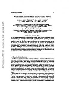
Chapter 2 Schemes for One-Dimensional Solids .... 2 ... ......................2.................4 0 ... ..1........ ..... . . .. . .... . . 0... ...E ... 3 .....".. .. .. . .. .. . . . . ..... .. ........... . . . . . . . . . . . . . . . . . . . . . ............. 6 ............. 5

Figure 2.1 Stress-strain relationship for an elastic-plastic material relationship is illustrated in Figure 2.1. The material is loaded starting from point 0. The stress-strain pair (; ") change according to Hooke's law until point 1, where the stress reaches the elastic yield limit 0. Then, the material undergoes plastic deformation. The slope of the curve in this range, Ep = d=d", is a function of the yield stress . At some point, point 2 for example, unloading takes place. (; ") decreases along the line from point 2 to 3, the slope of which is the same as Young's modulus E . The stress and strain will change in this line as long as jj 2. 2 is called the current yield stress in this range. If the loading is strong enough that exceeds the current yield stress, (; ") changes rst along the straight line to the point 2, and then changes along the plastic curve from point 2 to point 4. The Bauschinger eect is neglected. This means the condition for inverse yielding to take place is 2. The absolute value of slopes of the inverse plastic curve from point 5 to 6 will be the same as those from point 2 to 4. The above-mentioned constitutive relationship can be described by an incremental formulation. Suppose is the current yield stress, then 8 < d=E; when j + dj ; d" = : (2.4) d=Ep(); when j + dj > :

2.2.2 Lax-Wendro scheme Substituting eq. (2.3) into (2.1) to eliminate , we have the following equation @w = A @w ; (2.5) @t @x where ! ! u 0 E w= " ; A = 1= 0 :


23

Suppose the rod concerned is divided into nite cells along the x-axis with equal length x. Denote wjn = w(nt; j x) as the value in the cell center j at the time level tn. Then, taking Taylor's expansion for w(t; x) in (tn; xj ) up to the second-order: 2 2 wjn+1 = wjn + t @@tw nj + 2t @@tw2 nj : (2.6) If eq. (2.5) is substituted into (2.6), noting that A is a constant matrix, 2 2 wjn+1 = wjn + tA @@xw nj + 2t A2 @@xw2 nj : (2.7) The Lax-Wendro scheme [2.2] is derived when the derivatives in eq. (2.7) are replaced by central dierences: 2 (2.8) wjn+1 = wjn + 2 A(wjn+1 wjn 1 ) + 2 A2(wjn+1 2wjn + wjn 1); where = t=x. The use of scheme (2.8) requires calculation of the matrix A. This can be avoided by using the two-step Lax-Wendro scheme (the version of Richtmyer [2.3, 2.4]). To do this, we write eqs. (2.1) and (2.2) in another matrix form: @w = @f ; (2.9) @t @x where f = (; u)T. The rst step of the scheme calculates the values at grid point j + 12 at half time level tn+ 21 using the known values at time level tn, see Figure 2.2. The values of u and " are calculated by 1 wjn++122 = 12 (wjn + wjn+1 ) + 2 (fjn+1 fjn): (2.10) 1

1

With "jn++122 obtained in the above equation, jn++212 is calculated by eq. (2.3). Then we 1 have fjn++122 , which is called ux, in analogous to that in gas dynamics. The second step calculates the values at the cell center at time level tn+1. The values of u and " are obtained using the following formula 1

1

wjn+1 = wjn + (fjn++122 fjn+122 );

(2.11)

and again is obtained by eq. (2.3). For the linear problem, the two-step scheme is the same as scheme (2.8). But it is generally dierent for non-linear problems. Usually, the two-step scheme is used for computation, while scheme (2.8) is applied to stability analysis.

24

Chapter 2 Schemes for One-Dimensional Solids

second.......step ....

rst.. step ......... .......... .. . . . . . . . . n + 1....................................................................................................................................................................................................... ... .. . .. .. ... ... ... ..... ... ... .. .. .. ... ... ... ... .. .. ... .. t.. . . ... .... . . . . ... . . . .. n .................................................................................................................................................................................. .. j j 1 j+1 .. ....................... x t

t

t

Figure 2.2 A sketch for calculations using the Lax-Wendro scheme

2.2.3 Von Neumann condition and CFL number Using the nite dierence method to solve stress wave propagation gives a numerical solution to the problem. However, an error always exists between the numerical solution and the exact one. What is most important is whether the error will be bounded or not. If the error is bounded, the scheme is stable, otherwise it is unstable. The Fourier transform can be applied to the stability analysis. Let wjn be the error of wjn . De ne the function q by extending wjn to the whole cell region q(x; tn) = wjn; (xj x=2 x < xj + x=2): (2.12) Suppose q(x; tn) satis es the following condition: Z +1 kq(x; tn)k2dx < 1; (2.13) 1

where k k is the Euclidean norm: q kw(x; t)k ju(x; t)j2 + j"(x; t)j2: Then, q(x; tn) can be represented by the Fourier integral Z +1 1 n q(x; t ) = p2 1 q~ (k; tn)eikxdk; p where i= 1, and Z +1 1 n q~ (k; t ) = p2 1 q(x; tn)e ikxdx: When scheme (2.8) is used, the error at next time step is q(x; tn+1) = q(x; tn) + 2 A[q(x + x; tn) q(x x; tn)] 2 + 2 A2[q(x + x; tn) 2q(x; tn) + q(x x; tn)];

(2.14) (2.15) (2.16)

(2.17)


25

p

Multiplying eq. (2.17) by e ikx= 2 and then integrating with respect to x, noting that Z +1 1 p 1 q(x + x; tn)e ikxdx = q~ (k; tn)ei; (2.18) 2 with = kx, we obtain q~ (k; tn+1 ) = G() q~ (k; tn); (2.19) G() = I + i sin A + 2(cos 1)A2 ; (2.20) where I is the unit matrix, and G is called the ampli cation matrix. Introduce the norm of matrix G by kGk sup kGqk (2.21) kqk : Since

if kGk 1,

kqk6=0

kq~(k; tn+1)k2 = kGq~(k; tn)k2 kGk2 kq~(k; tn)k2;

(2.22)

kq~(k; tn+1)k2 kq~ (k; tn)k2:

(2.23)

Using Parseval's equivalence relation Z +1 Z +1 kq~ (k; tn)k2dk = kq(x; tn)k2dx; we have

1

Z +1

1

kq(x; tn+1)k2dx

Z +1

(2.24)

kq(x; tn)k2dx;

(2.25) which means that the error is bounded during the computation, and the scheme is then stable. kGk 1 can be used as a de nition for stable schemes. Denote the eigenvalues of matrix G by %(G). According to matrix theory, the absolute maximum of the eigenvalues satis es max j%(G)j kGk: (2.26) Therefore, a necessary condition for stable schemes is all j%(G)j 1. Usually, this is called the von Neumann stability condition. According to eq. (2.20), the eigenvalues of matrix G can be obtained from those of the matrix A by 1

1

%(G) = 1 + i sin %(A) + 2(cos 1)[%(A)]2: (2.27) q %(A) is easily calculated as c0, where c0 = E= is the longitudinal wave speed in the rod. Therefore, %(G) = 1 ic0 sin + (c0)2(cos 1):

(2.28)

26


If c0 1, the von Neumann condition is satis ed. c0 is called the Courant-FriedrichsLewy (CFL) number. In many computational cases of stress wave problems, von Neumann stability condition is also a sucient condition. Let us use the dimensionless variable w = (u=c0; ")T in eq. (2.5). We know such a transformation will not change the properties of numerical scheme. Then the matrix A becomes ! 0 c 0 A = c0 0 : (2.29) Hence, G in eq. (2.20) becomes a normal matrix (GTG = GGT, where G is the conjugate matrix of G). According to matrix theory, we have kGk = max j%(G)j. Therefore, c0 1 is the also the sucient condition for stable computation.

CFL = 0:9; x = 0:01 CFL = 0:9; x = 0:1........... ...... . ................. CFL = 1 ....................................................................................................... ... .. .. .. .. .....

1.5 1.0

0.5 0.0 0:5

................

.........

... ... ... ... ... ... ... .... ... .... ......... ..... ..... .... .... ..... ... ... . ...... . ................................................................................

...... ...... . ........ ........ .. .. ... . . ..... .... ... ... . . ...................................................................................................... ......... .... ... ..

8

9

Time = 9

x

10

11

Figure 2.3 Results by Lax-Wendro's method for a one-dimensional elastic wave with dierent CFL numbers One of the most important features in solid dynamics is the correct reproduction of the wave structure after impact. Generally, the characteristic time of the contact of a drop hammer with the specimen reaches only a few or some tens of micro-seconds. During this time a very complicated wave structure with several dierent amplitudes is initiated. The amplitude of the elastic precursor produced by an impact is high, but its wave length is very small compared with the scale of the specimen. A rst-order nite dierence scheme is not able to reproduce this kind of wave correctly because the scheme's numerical dissipation is too large and will atten the wave front arti cially. Therefore, a higher-order accurate method should be used. The necessary stability


27

condition of many explicit numerical solvers of hyperbolic PDEs, e.g. the Lax-Wendro scheme discussed above, is CFL 1. But in order to preserve the physical wave pro le correctly, this number has to reach 1 in the limit. For example, let us consider a onedimensional elastic wave in the rod. Suppose eqs. (2.1) to (2.3) are valid in 1 < x < 1 with = 1, E = 1, and the following initial conditions given at t = 0: ( < x < 1; = u = 10;; when 0otherwise (2.30) : This kind of a rectangular wave pro le is an idealized model for an impact. Figure 2.3 shows the results obtained by the Lax-Wendro scheme for CFL=1 and CFL=0.9. It can be seen that using CFL=1 is more accurate.

2.2.4 Elastic-plastic problems When the Lax-Wendro scheme is applied to an elastic-plastic problem, a serious dif culty arises. First, 1u and " are calculated by eq. (2.10). However, eq. (2.4) is not n+ 12 n+ 2 applicable to get j+ 12 with the obtained "j+ 12 , because the yield stresses nj and nj+1 and the related function Ep() may be dierent. This can cause plastic loading in one cell 1and elastic unloading in an adjacent cell at the same time. But the ux component jn++122 is needed in the second step to update the solution. ..... t ... .. . .. .... ..... .... .. ..... .... ... .. ...... ..... .... ... .. .. ...... .... .... ... .. .. ...... ..... ... ... ... ...... ..... .... ... .. . ...... .... .... ... .. 3 .. 4 ...... ..... .... ... .. .. ...... ..... .... ... .. . ...... .... .... ... ... .. .................... . .................... .. 1 2 ................ . .......... .. .....................................................................................................................................................................................................................

........ .. . . . . . ........ . . ..... . ........ . . . . . . ........ ..... . . . . . ........ . . ........ ............. ...... ..............................

u1

rod 1

... ... ... ...

.............................

x

u2 rod 2

Figure 2.4 Riemann problem in (x; t) plane arised in the impact of two rods Such a strange situation does not occur in gas dynamics, because in that case the equation of state is an algebraic one. In order to overcome the diculty, let us consider

28


the basic impact phenomenon of two rods, see Figure 2.4. Suppose the initial states of two rods are u1; 1; "1 and u2; 2; "2. After impact, two families of centered simple waves will arise, one family propagating into the left-hand rod, and another into the righthand rod. Depending on the initial values in the two rods and the material properties, these waves can be either elastic shock (in both loading and unloading cases) or plastic continuous loading disturbances. The boundary conditions for the solution are: the stress and velocity components in the interface should be equal, i.e. 3 = 4, u3 = u4. As for the strain in the interface, "3 6= "4 is possible which corresponds to a contact discontinuity in gas dynamics. Such a problem is called a Riemann problem. The real physical process can be applied to numerical computation in the interface of two cells. Instead of calculating the strain component ", the stress and velocity components will be calculated in the rst step by solving a Riemann problem described above. This is the well-known Godunov method [2.5].

2.3 Godunov's method for rods 2.3.1 Simple wave solution In order to deal with the elastic-plastic problem, it is convenient to write the stressstrain relationship (2.4) by the formula h d; (2.31) d" = 1 + E where h = h() is called the plastic factor: 8 < 0; when j + dj ; h=: (2.32) E=Ep() 1; when j + dj > : Substituting eq. (2.31) into eq. (2.9) to eliminate ", the equation

@f A @@tf = @x is obtained, where

! 0 A = (1 + h)=E 0 ;

(2.33)

! f= u :

Suppose the centered waves produced by an impact emanate from the origin of the (x; t) plane, see Figure 2.4. Since the initial regions 1 and 2 are in homogeneous states,

2.3 Godunov's method for rods

29

the simple wave solutions can be found for eq. (2.33), for which f is a function of c = x=t only: f = f (c). Therefore, eq. (2.33) can be rewritten as (cA + I)df = 0;

(2.34)

where c is a free parameter. But c must satisfy the following equation for a non-trivial solution df 6= 0 to exist: det (cA + I) = 0; (2.35) where det stands for the determinant. Solving this equation for c gives the characteristic wave speed: s (2.36) c = (1E+ h) :

In the elastic range h = 0, then c = c0; in the plastic range h 6= 0, then c is a function of the yield stress . For decreasing work-hardening materials, Ep() E , i.e. h 0. Therefore c() c0: (2.37) The solutions of eq. (2.35) for c contain the + sign for rightward running waves and the sign for leftward running waves. In the rightward simple wave region: x=t = c (x > 0), where c may assume the values of c0 or c(), the non-trivial solution df of eq. (2.34) results in the following compatibility relation: (2.38) du = dc : The compatibility relation for the leftward wave region (x < 0) is obtained by simply changing the sign for c in the above equation.

2.3.2 Riemann solver and Godunov's method We now solve the Riemann problem shown by the sketch in Figure 2.4. eq. (2.38) to the leftward wave region (x < 0) from state 1 to state 3, Z 3 d u3 = u1 + : 1 c() In the same way, from state 2 to state 4 in the rightward wave region, Z 4 d u4 = u2 : 2 c() The boundary conditions for the solutions are

u3 = u4; 3 = 4:

Applying (2.39) (2.40) (2.41)

30


After eliminating u3 and u4 from eqs. (2.39) and (2.40), Z d Z d + =u u ; (2.42) 1 c() 2 c() 2 1 where = 3 = 4 is used in the upper limits of the integrals. Equation (2.42) can be used to calculate by an iterative method. The two wave speeds c() inside the integrals are obtained from the loading history in the rod from state 1 to 3 (or from state 2 to 4). Following is the iterative procedure that can be used to nd : (i) Put both c() = c0, by which eq. (2.42) gives the elastic result: = 12 (1 + 2) + c20 (u2 u1): (2.43) (ii) If does not exceed the current yield stress in both rods, i.e. jj 1, jj 2, then is the solution. Otherwise, the linearization is taken for eq. (2.42) at point ^ , and Newton's iterative method is applied to the work: 1 Z ^3 d Z ^4 d 1 + =u u ; (2.44) ( ^ ) c^ + c^ + 1 c() 2 c() 2 1 3 4 where ^3 = ^4 = ^ , but c^3 6= c^4 in general, since c^3 depends not only on the current stress ^ , but also on the loading history from state 1 to state 3 (similarly, c^4 depends on the history from state 2 to state 4). In the rst iterative cycle, ^ is set to the elastic result. The iteration will be carried out until converges. (iii) When is obtained, u3 (= u4) is calculated by eq. (2.39). One can also calculate "3 and "4 at the interface. However, the strain components in the Riemann solution are not used in the numerical work. Therefore we do not discuss them. Godunov's method [2.5] also involves two steps. Suppose at time level t = tn the functions f (x; tn), (x; tn) are represented by a set of homogeneous values in cell j : fjn, nj . Depending on the function distribution, dierent cells may have dierent states. Therefore, when t > tn , a series of Riemann problems occur along the interfaces between the cells. Solving the Riemann problem with the initial values in cell j and cell j +1, the solution can be obtained fj+ 12 in the interface j + 12 . This is the rst step in Godunov's method, In the second step, integrating for eq. (2.9) over the area S fjx xj j x=2; tn t tn+1g, ZZ @ w @ f 0 = @x dxdt S @t xZj+ 12 xZj+ 12 tZn+1 tZn+1 = wn+1 dx wjndx fj+ 12 dt + fj 12 dt: (2.45) n n xj 12 xj 12 t t


Since wjn , fj+ 12 and fj ing:

1 2

31

are constants, the above equation gives the schemes for updat-

wjn+1 = wjn + xt (fj+ 21 fj 12 ):

(2.46)

where wjn+1 is the integral average of the solution. With the result "nj +1 in wjn+1 , the stress jn+1 and yield stress nj +1 can be calculated by the elastic-plastic relationship (2.4). The eq. (2.46) is identical to eq. (2.11). However, since it is deduced by the integral method, the conservation of mass and momentum is insured and the scheme is correct even when shock waves arise in the cells. Since the uxes fj+ 12 and fj 12 need to be constant on the cell's interfaces, t in eq. (2.46) must be set to be small enough to insure that during this time the wave disturbances generated in one interface do not propagate over x to reach the neighboring interface. According to eq. (2.37), the CFL number is again obtained as c0t=x 1. In many problems boundary conditions are given. The boundary coincides with one interface of the adjacent cell, where only one component (either or u) can be prescribed, while the other component is calculated by the Riemann invariant (2.38). If the rod has a left boundary, the impact on the boundary will result in a rightward wave propagating into the rod. Then eq. (2.40) can be applied to calculate the boundary condition.

2.3.3 The second-order Godunov scheme The Godunov method discussed above oers a physically reasonable treatment of elasticplastic wave propagation. However, the scheme is only rst-order accurate. To prove this statement, Godunov's method is applied to the elastic case. The ux can easily be found to be fj+ 12 = 12 (fjn + fjn+1 ) + c20 (wjn+1 wjn ): (2.47) Substituting the ux into eq. (2.46), and then letting x ! 0, @ f n c0t @ 2w n wjn+1 = wjn + t @x + 2 @x2 j x: (2.48) j Comparing this expression with eq. (2.7), it can be seen immediately that the error begins in the term of the second-order derivative. In order to obtain a second-order accurate scheme, let us examine the most simple situation sketched in Figure 2.5, where the distribution of stress is assumed as a solution of the Riemann problem at t = tn + t=2. In the rst-order Godunov method, fj+ 12 is the value at the interface x = xj+ 12 . It becomes evident from the pro le in

32


............................................................................................................................... ... .. ..... .. .......... ........................................................ .... t ......... .. .. ......... .. . ................... .. . . . . .. .. .. .. ... ... .......... . .. . . . .. ... .. .. .. ... ............ .. . .. .. .. .. ... .... . .. .. .. .. ....... 1 t .... .. .. ........... .. .. ............. 2 .. .. ............. .. .. ............. .. .. ........... .. ..... . . . ...............................................................................................................................................................................................................................................................

j

...... ... . . ...... . . ...... .... . . . . ...... .... . . ...... . . ...... .... . . . . ...... .... . . ...... . . ...... ........ ..

j+1

0

1 x 1 x . . ... . ..............................................2..............................................................................................................2................................................................

x

Figure 2.5 A sketch for constructing a second-order Godunov method Figure 2.5 that much information in the Riemann solution can be lost by this way. In gas dynamics, Glimm [2.6] used a random number to select the solution point. Van Leer [2.7] and later Ben-Artzi et al [2.8] achieved second-order accuracy by reorganizing a linear distribution for the initial values, and solving a general Riemann problem. The method to be introduced here has been developed by Toro [2.9], and Lin and Ballmann [2.10], for which the construction of the second-order scheme can be formulated directly from the Riemann solution. In this method, the ux fj+ 21 in eq. (2.46) is replaced by its integral average in two half cells, i.e., Zx f j+ 12 = 1x x j+1 f dx; (t = tn+ 12 ): (2.49) j Since the wave speed c is known for the solution of the Riemann problem, eq. (2.49) can be rewritten in a more practical form. Assuming xj+ 12 as the origin, integrating eq. (2.49) by parts, and noting x = ct=2 for x < 0 and x = ct=2 for x > 0, we then have fZj+ 12 fZj+ 12 1 t f j+ 12 = 2 (fjn + fjn+1) + 2x ( c df + c df ): (2.50) n n

fj

fj+1

The scheme (2.46) with the ux (2.50) will possess second-order accuracy in domains of smooth solution. In order to prove this, we use eq. (2.34) to rewrite eq. (2.50) in the


33

approximate form: t A 1 (f n f n ); f j+ 12 = 12 (fjn + fjn+1 ) + 2 x j+ 2 j+1 j

(2.51)

where A = A 1. Substituting eq. (2.51) into eq. (2.46) we would arrive at the original Lax-Wendro scheme. It is interesting to note that one component of the second-order ux, i.e. uj+ 12 can be written in a closed form. Since eq. (2.38) is valid in a simple wave region, it can be substituted into the rst equation of eq. (2.50) to give uj+ 21 = 12 (unj + unj+1 ) + 2tx (jn+1 jn): (2.52) This is equivalent to the Lax-Wendro scheme. The simplicity of the expression for u is a consequence of the fact that the rst equation in eq. (2.33) is linear. The numerical procedure consists of three steps: the rst one is to solve the Riemann problem, and to get the solution for the fan-shaped simple wave regions on both sides of the interface; the second one is to calculate the ux by eq. (2.50); the nal step is the updating of wjn+1 by eq. (2.46) and the calculation of and .

2.3.4 A test example As a test example, we consider a semi-in nite rod which obeys a linearly elastic, powerlaw work-hardening plastic stress-strain relationship given by 1 = 1: (2.53) Ep() E 0 The material parameters are taken as = 1, E = 1, 0 = 1, = 3. The rod is at rest before t < 0, i.e. the initial conditions for both u and are set to zero. The boundary condition at x = 0 is described by the following rectangular impact loads: 8 < 3; when 0 t 2; (t; 0) = : (2.54) 0; when 2 < t < 1: This kind of problem was considered by Bohnenblust [2.11]. The solution can be obtained analytically using the method of characteristics. In the (x; t) plane, see Figure 2.6, an elastic precursor and a family of centered plastic waves are emitted from the origin when the sudden impact is applied there. The elastic precursor (line 0a) propagates with wave speed c0 = 1. Because of the plastic wave speed c() = 1=(p), the rst plastic disturbance (line 0b) propagates with c = 1=p, while the last disturbance

34


9 8 7 6

t

5 4 3 2 1 0

a a a a a a a a a a a a a a a a a a

a a

0

a aa aa a a a a a a a a a a a a a a a a a a a a a a a a a a a a a a a a a a a a a a a a a a a a a a a a a a a a a a a a a a a a a a a a a a a a a a a a a a a a a a a a a a a a a a a a a a a a a a a a a a a a a a a a a a a a a a a a a a a a a a a a a a a a a a a a a a a a a a a

1

2

x

2

...

. .. .. . . . .. . . .. .. ....... . . . .. ..... b .. .. ............ . . . . . .. .... . .. .. . .. .. ....... ..... . . . . . . .. .... .. .. .. .. .. ....... ..... . . . . .. ... . .. .. .. ....... ..... .. . . . . .. ... . .. . ... .. .. ...... . . . . .... . . .. ... .. .. ... .. .. ....... . . . .. .. . . . a. ... .. .. .. ... ..... .. . . . . . . .. .. . . . . . . . . . . . . . . .. . ... .. . ... .... ... .. .. . . . . . . . . . . . . . . . .. ... ..... . e ...... .. .. . . .. .. ..... .... .. .. .. . .. ...... .. .. ... ... . . . . . . . . . . . . . .. ... . . ...... ... .... .. . . .. ..c.......... d .... . .. . . ...... ... .... .. .. . . . . . .... ... ... ..... .. . ... .. ... . . .. . .. .. .... .. .... .. .. .. .. .. .... .... ..... .... .. .. .. . ...... .... ........... .. .... . . .. .. .. . . . ...

3

4

5

1 0 3

t=4 ............. ... ......... ....... .. ........................................ .. . . ... . . .. .........

aa a aaa aa a aa a aa aa a aa aaa a aaa a aaa aaa a aaaaaaaaaaaaaaaaaaaaaaaaaaaaaaaa a a a a aa a a aa aa a a aa aaaaaa

...... .. ... .. ... .. .... .. ... t=2.4 .. ... .. .... .... .. ...... .. ............................... .. ... .. ... .. ... . . ............ a a a

a

2 1 0 3

a a a a a a a a a a aa aa aa aa aa aaaaaaaaaaaaaaaaaaaaaaaaaa

aaaaaaaaaa

aaaaaaaaaaaaaaaaaaaaaaaaaaaa

............. ... ... ... ... ... ... ... .... ............................ ... ... ... ... .. aaaaaaaaaa

a

a

2 1 0

a a a a a a a a a a aa aa aa aaaaaaaaaaaaaaaaaaaaaa

0

1

t=2

aaaaaaaaaaaaaaaaaaaaaaaaaaaaaaaaaaaaaa

x

2

3

Figure 2.6 The numerical results (circle) for the elastic-plastic boundaries in (x; t) plane and stress distributions at given time t, compared with the exact solutions (solid lines). Some important characteristic lines are also drawn in the (x; t) plane by dashed lines

p

(line 0c) propagates with c = 1=(3 ). Behind line 0c is a constant region. When the loading is suddenly removed from the left boundary at t = 2, an elastic unloading wave propagates with c0 = 1 into the rod to unload the plastic yield region. This unloading wave is also an elastic-plastic boundary, behind which is an elastic region where the characteristic wave speed is c0. The unloading elastic-plastic boundary begins as a strong discontinuity, across which and u have to jump. But the jump ends at point d. Then, the unloading disturbance takes place along a weak discontinuous boundary which is not a characteristic line beginning from point e. Later, the unloading boundary catches up with the loading boundary at point b. The plastic wave propagation is nally terminated.


35

We have taken the numerical modeling for the above-mentioned wave propagation problem by the second-order Godunov method. The elastic-plastic boundaries in the (x; t) plane are drawn by plotting the traces of the rst plastic wave (de ned by =0 = 1:01 and the elastic unloading wave (de ned by ( jj)=0 = 0:05). It is seen that the numerical results coincide well with the exact solution, except for one part of the unloading boundary at x = 0, on which the centered wave solution behaves as a singular phenomenon. The stress distributions for three dierent time levels are also plotted in Figure 2.6. They also agree well with the exact solution.

2.3.5 A computer program In order to show the working procedure of the second-order Godunov's method, a FORTRAN computer program for above test problem is listed below. c*********************************************************** program WAVE1D c----------------------------------------------------------c This program is used to model the Elastic-Plastic Waves c in one-dimensional rods. (alpha=1/en) parameter (ke=1000,nmax=900) dimension s(ke),u(ke),e(ke),f(ke),mf(ke) real time(0:nmax),xl(nmax),xr(nmax) real sr(0:ke),ur(0:ke), st(3),ut(3),ft(2) common/mate/ rho,c0,fk0,en rho=1.0 c0 =1.0 fk0=1.0 en =1./3. dx=0.01 dt=dx/c0

10

do 10 k=1,ke s(k)=0. u(k)=0. e(k)=0. f(k)=fk0 mf(k)=0 continue time(0)=0. do 900 n=1,nmax

36

Chapter 2 Schemes for One-Dimensional Solids write(*,*)' n=', n

c----------- Riemann problem for flux ---do 100 k=1,ke-1 st(1)=s(k) ut(1)=u(k) ft(1)=f(k) st(2)=s(k+1) ut(2)=u(k+1) ft(2)=f(k+1)

100

call riem(st,ut,ft) sr(k)=st(3) ur(k)=ut(3) continue

c------------ left boundary condition ---call left(n,dt,simpt) sr(0)=simpt ur(0)=u(1)+dt/(rho*dx)*(s(1)-simpt) c------------ right boundary condition ---sr(ke)=0. ur(ke)=u(ke)+dt/(rho*dx)*(0.-s(ke)) c------------ updating -------------------time(n)=time(n-1)+dt do 200 k=1,ke u(k)=u(k)+dt/(rho*dx)*(sr(k)-sr(k-1)) de=dt/dx*(ur(k)-ur(k-1)) e(k)=e(k)+de sig=s(k)+rho*c0*c0*de if (abs(sig).lt.f(k)) then s(k)=sig test=(f(k)-abs(sig))/fk0 if ((mf(k).eq.1).and.(test.gt.0.05)) mf(k)=2 goto 200 end if sa=f(k) if (sig.lt.0) sa=-sa de1=de-(sa-s(k))/(rho*c0*c0) nk=5.+abs(de1)*rho*c0*c0/fk0*200. dde=de1/float(nk) do 150 i=1,nk


150

200

300

950

ff=abs(sa) ep=en*rho*c0*c0*(ff/fk0)**(1.-1./en) sa=sa+ep*dde continue s(k)=sa f(k)=abs(sa) if ((mf(k).eq.0).and.((f(k)/fk0).gt.1.01)) mf(k)=1 continue xl(n)=0. xr(n)=0. do 300 k=1,ke if (mf(k).eq.2) xl(n)=k*dx if (mf(k).eq.1) xr(n)=(k-1.)*dx continue if ((n.eq.200).or.(n.eq.240).or.(n.eq.400)) then nput=n/10 write(nput,*) ' One-dimensional rod problem' write(nput,*) ' Stress distribution at t=',time(n) do 950 k=1,350,4 write(nput,1100) (k-0.5)*dx, -s(k) continue end if

900

continue

910

write(12,*) ' Elastic-plastic boundary, loading, 0.01 ' write(14,*) ' Elastic-plastic boundary, unloading,0.05 ' do 910 n=1,nmax,10 if (xl(n).gt.0.03) write(14,1100) xl(n),time(n) if (xr(n).gt.0.03) write(12,1100) xr(n),time(n) continue

1100

format(2f7.3,' *1 0 0') end

c*********************************************************** subroutine riem(s,u,f) c----------------------------------------------------------c A subroutine for solving Riemann problem. c The output is the second-order flux. real s(3),u(3),f(2),ss(2,1010),cc(2,1010)

37

38

Chapter 2 Schemes for One-Dimensional Solids dimension nn(1010) common/mate/ rho,c0,fk0,en

c----------- when CFL=1, c0=dx/dt. ---------------------u(3)=(u(1)+u(2))/2.+(s(2)-s(1))/(2.*rho*c0) s(3)=(s(1)+s(2))/2.+rho*c0*(u(2)-u(1))/2. sig=s(3) if ((abs(sig).le.f(1)).and.(abs(sig).le.f(2))) return

1

en1=(en-1.)/(2.*en) do 200 m=1,2 ss(m,1)=s(m) cc(m,1)=c0 if (abs(sig).le.f(m)) then ss(m,2)=sig cc(m,2)=c0 nn(m)=2 goto 200 end if sa=f(m) if (sig.lt.0) sa=-sa ss(m,2)=sa nk=5+(abs(sig)-f(m))/fk0*200 if (nk.gt.1000) nk=1000 ds=(sig-sa)/float(nk)

100

do 100 i=1,nk ss(m,i+2)=sa+float(i)*ds ff=abs(sa+(i-0.5)*ds) cc(m,i+1)=c0*sqrt(en)*(ff/fk0)**en1 continue

200

ff=abs(ss(m,nk+2)) cc(m,nk+2)=c0*sqrt(en)*(ff/fk0)**en1 nn(m)=nk+2 continue

300 310

sum=u(2)-u(1) do 310 m=1,2 do 300 i=1,nn(m)-1 sum=sum-(ss(m,i+1)-ss(m,i))/(rho*cc(m,i)) continue continue rr=1./(rho*cc(1,nn(1)))+1./(rho*cc(2,nn(2)))

2.4 Combined stress waves in a thin-walled tube

39

sum=sig+sum/rr if ((abs(sum-sig)/fk0).le.1e-6) goto 500 sig=sum goto 1 500

560

s(3)=s(1)+s(2) do 560 m=1,2 do 560 i=1,nn(m)-1 s(3)=s(3)+(cc(m,i)/c0)*(ss(m,i+1)-ss(m,i)) continue s(3)=s(3)/2. return end

c*********************************************************** subroutine left(n,dt,simpt) c----------------------------------------------------------c left boundary condition common/mate/ rho,c0,fk0,en t=float(n)*dt if (t.le.2.0001) then simpt=-3.*fk0 else simpt=0. end if return end

2.4 Combined stress waves in a thin-walled tube 2.4.1 Governing equations

In solids, two or three stress components usually exist in a sectional surface. One simple model is the thin-walled tube which is subjected to a combined longitudinal and torsional shock loading, see Figure 2.7. It is evident that there are two stress components and two velocity components in the sectional surface. The stress wave propagation in the tube contains both a longitudinal wave and a torsional wave. If the material is linear elastic, the governing equations are linear. Then the solutions can be

40


obtained by means of superposition for the two waves. However, the situation becomes more complicated when plastic ow occurs in the material. In such a case, the two stress components are related to each other since they must jointly obey a given yield condition. Therefore we will observe combined longitudinal and torsional waves in the tube. ... ........................................................................................................................................................... . . . . . . ....................... .......................................................... . ......... ......... ......... ......... ....... . ......... ......... ......... ......... ......... ................ ...................................x.. ... ............. . . ... . .................................................................................................................................................................... .... ..

Figure 2.7 Thin-walled tube subjected to a sudden combined loading (; ) It is very important to understand the basic properties of the combined stress waves in order to model them numerically. Following [2.12{2.15] for the derivation of the system of PDEs to be solved, we start with the local balance of momentum in the longitudinal direction and circumferential direction, and the linearized strain-displacement relations partially derived with respect to time: @w = @f ; (2.55) @t @x where 0 u 1 01 B C B C w = BB@ v" CCA ; f = BB@ u CCA :

v u; ; " shall represent the longitudinal particle velocity, stress and strain, and v; ; the corresponding circumferential quantities; is the mass density, t is the time, and x is the distance measured along the axis of the tube. The material of the tube is assumed to be isotropic and work-hardening. The strain increments contain an elastic part and a plastic part: d" = d"e + d"p; d = d e + d p: (2.56) The elastic part obeys Hooke's law (2.57) d"e = E1 d; d e = 1 d; where E is Young's modulus and the shear modulus. The increments of plastic strains may be obtained with a scalar plastic potential ' p = @' d; d"p = @' d ; d

(2.58) @ @


41

where d is a positive multiplier, possibly dependent on the history of irreversible deformation. The plastic potential ' is usually taken as the yield function, which has the following form under the combined stress loading condition in a thin-walled tube: 2 (2.59) ' + 2 2 = 0;

p

with = 3 for the von Mises yield condition and = 2 for the Tresca yield condition, is called the yield stress (The value of here is dierent from that in Section 2.2 by a factor ). Therefore, (2.60) d"p = 22 d; d p = 2 d:

In order to determine the multiplier d, the ow rule of eqs. (2.60) is applied to a one-dimensional simple tension test, where = , = 0; then ! ! 1 1 1 1 p d" = g() E d = g() E d; (2.61)

where g()=d/d" is the slope of the stress-strain curve in simple tension. The multiplier d is then found by comparing the two d"p in eqs. (2.60) and (2.61), ! 2 1 1 (2.62) d = 22 g() E d: The value d is obtained from eq. (2.59). Then the increments of plastic strain components are determined from the stress components. Summarizing the above discussion, the stress-strain relationship can be written as follows: 2 d" = E1 + H 2 d + Hd; d = H d + 1 + H2 2 d; (2.63) with the function H de ned by 1 H = 12 g( )

! 1 : E

(2.64)

H is double-valued. In the elastic case, g() = E , so H = 0; but H 6= 0 in the plastic case since g() < E . It should be noted that the constitutive relations (2.63) are nonlinear even for linearly work-hardening materials: g() = Ep (constant).

42


2.4.2 Characteristic relations Substituting eqs. (2.63) into eq. (2.55), the governing equations can be rewritten as @f ; A @@tf = @x (2.65) where 0 0 0 01 B 0 0 0 C B CC B 2 B CC : 1 H A = BB + 2 H 0 0 CC B @E 1 2 2 0 0 A H + H

For eq. (2.65) a simple wave solution can be found which connects two domains of dierent homogeneous states. In this case f is a function of x=t = c only. Eq. (2.65) is then rewritten in the form (cA + I) df = 0; (2.66) where c is a free parameter. A necessary condition for a non-trivial solution df 6= 0 to exist, is D(c) det(cA + I) = 0: (2.67) Expanding the determinant, D(c) has the following form: h 2 ih c 2 i D(c) = cc 1 c 1 0 2 h c 2 i 2 h c 2 i 2 2 2 + c H 1 2 + c 1 ; (2.68) c2 0 where s s E (2.69) c0 = ; c2 = : Therefore, in the elastic case (when H = 0), the solutions for D(c) = 0 are c = c0 and c = c2, which are the characteristic wave speeds for the longitudinal wave and the torsional wave in the linear elastic tube, respectively. In the plastic case, the solutions for c are correlated with the stresses (; ). Because D(0) > 0, D(c2) < 0, D(c0 ) > 0 and D(1) > 0, there are also two roots for D(c) = 0. If one is denoted by cs and another by cf , they should satisfy 0 cs c2 cf c0:

(2.70)

The wave speeds cs and cf are distinguished as slow and fast. The solutions of eq. (2.67) contain the + sign for right-running waves and the sign for left-running waves.


43

In the rightward simple wave region, x=t = c (x > 0), where c may assume the values of c0; cf ; c2 or cs , eq. (2.66) results in the following compatibility relations: du = d ; dv = d ; (2.71) c c c 2 1 d = c2 (2.72) d c 2 1 2 (c): c0 The compatibility relations for the leftward wave region (x < 0) can be obtained by simply changing the sign of c in the above three equations.

2.4.3 Loading path in stress space It becomes evident that the compatibility relation (2.72) is a restriction for the stresses and under combined tension and torsion. This relation does not depend on the velocity components. Therefore, if the initial state and nal state for (; ) are given, eq. (2.72) can be integrated to obtain a curve = ( ) connecting these two states. In the (; ) plane, such an integral curve is called the stress loading path, or simply the loading path. ... .... cs .. .. ........ ............ . . ... ................................c.. ....... ......... .............. cf . . . . . . . . . ...... . .. .. .. 2 .... .. ........................ c0 .... .. .. ........................................................................................................................................................................... . .. ... ... .. . . . . . . . . ........ .. ................................... ................. .. .. .. .

Figure 2.8 The directions of loading paths in (; ) stress space Let us analyze some details of the loading path. For a given stress state (; ), two characteristic wave speeds for c can be obtained by eq. (2.67). Then there are two (c) in eq. (2.72), which correspond to the two directions of the loading paths in the stress plane. Suppose, see Figure 2.8, the elliptical curve is the initial yield surface represented by eq. (2.59). The given stress state is located in the region 0, 0. In elastic region, i.e. the point (; ) is inside the yield surface, the characteristic wave speeds are c0 and c2. Eq. (2.72) shows in this case that the stress paths are straight lines parallel

44


to the -axis or -axis. In the plastic region, i.e. the point lies on a current yield surface and causes this surface to become larger, the two wave speeds are c = cf and c = cs. Eq. (2.72) shows that (cf ) 0, which means along the cf -path increases but will decrease. Whereas, (cs) 0 means that both and will increase along cs-path. A further analysis shows (cf ) (cs) = 1. This means the two families of loading paths are perpendicular to each other everywhere. Although there are always two possible loading directions for any given point in the (; ) plane, the true physical process takes only one direction which can be determined by the loading conditions. Let us consider an example: a pre-stressed semi-in nite tube is subjected to a sudden combined tensional and torsional impact at the left boundary. The pre-stressed state, denoted by (i; i), lies inside the initial yield surface characterized by i. The nal state after impact, is denoted by (^; ^), is outside the surface i . The disturbances caused by the impact will propagate into the tube with the wave speeds listed in eq. (2.70). Since c0 is the highest wave speed, this wave (if it exists) should run the fastest. Then a cf -wave follows, and later a c2-wave. The last wave is a cs -wave. Therefore, the nal state (; ) can be considered to be reached after a cs -wave. Taking = (cs) to obtain an integral curve through (^; ^) by eq. (2.72), we have two cases. Case 1: As shown in Figure 2.9, the value ^ is not too large. The cs -path reaches the initial yield surface at point 2. Since point i and point 2 may be connected by two elastic paths, i.e. c0-path and c2-path, the cf -path does not exist. According to this loading pattern, the characteristic lines in the (x; t) plane contain one c0-wave, one c2-wave and one family of cs -waves. Case 2: See Figure 2.10, ^ is high enough that there is no connecting point for the cs -path and the initial yield surface. Then the tube will rst be loaded along a c0-path to the i surface, and followed by a cf -path to connect the cs -path. The c2-path does not exist in the physical process because c2 cf . Accordingly, the (x; t) plane contains one c0-wave, one family of cf -waves and one family of cs-waves.

The conclusion to this section is: for a thin-walled tube with two stress components in the sectional surface, the stress must be loaded along a certain stress loading path in the order of c0 ! cf ! c2 ! cs. Among them the c0- and c2-paths appear only inside the yield surface, while the cf - and cs -paths appear on the current yield surface.

2.5 Numerical modeling of combined stress waves

(^; ^)

.... ... .. .... . . .i..................................................2........................ . .. c2 . .. ... .. i......................... 1 ..... .. .. . . c .....................................................................................................0..................................................................... ... . .. .. ... . . . . . .... .. ..... .... . . . ........ ...................... ........ . . . . . .. .. ..

cs c2 .... t .. . ... ... ... . .. (^ . . ... ... .. ; ^) ... .... ..... ..... .. . .. ... ... 2 .. .. .............. . .. . .. ........ . .. . . ...... .. ................ . 1 .. ........... c0 .. ............. .. ............ .. ......... ......... ........................................................................i.................................................................................

... . . . . .... . . . . .... . . . . .... . . . . .... . ....... . . . . . . . . . . . . . . . . . . . . . ................................. . . . . . .... 0 .........

45

x

Figure 2.9 A sketch of the loading path in the (; ) stress space and the corresponding characteristic lines in the (x; t) plane for the small ^ ... (^;.^) .. ... . i ............... ............................................................................1....... cf cs .... ................ . .. .. . ... ........ . ..... .. i c0 ... .. . . .. ... 3 . .......................................................................................................................................................................... ... . .. ... ... . . . . .... .. ... .. .... . . ......... ......................... ....... . .. .. ... .. 0

cs ..... t .. . ... ... ... . .. (^ . . ... ... .. ; ^) ... .... ..... ..... ... .. . .. ... ... ...................cf . . . . .. . .............. 3 . .. ..... ..... ...... .. .. . .. ... ... ................................................... . . . . . .. .. ............... . ............................ . . ...... .. .................................................. . . . . .. ................. .. . . c0 .. ............ ..................................................... 1 .. .............. .................................... .. .......... .................... .. ........................ ...........................................................................i.................................................................................

...... . . . . . . . . . . . . . . . . .......... . . . . . . . . . . . . . . . . .................

x

Figure 2.10 A sketch of the loading path in the (; ) stress space and the correspond characteristic lines in the (x; t) plane for a large ^

2.5 Numerical modeling of combined stress waves 2.5.1 Riemann problems Let us suppose the initial conditions at t = 0 are two dierent homogeneous states, and the initial states are denoted by f in x < 0 and f+ in x > 0, respectively. When t > 0, two families of centered simple waves will arise, one family propagating to the left-hand side, and another to the right. Depending on the initial values in the two wave regions, the wave speeds in the two wave families may take on all values occurring in eq. (2.70), or only some of them, i.e., any one or two or three or four of the dierent kinds of waves may be absent. As an example, one possible con guration of simple waves for certain given initial conditions is sketched in Figure 2.11. Following a line x=constant advancing in time, the waves which occur can be crossed only in the inverse sequence as

46


written in eq. (2.70). This fact helps us to nd a rule for the loading path in the stress space to be used in the Riemann solver, as will be discussed in the next two subsections. Here, we want to get the solution f at the interface: x = 0; t > 0. .... t c .. . .. . s . .. .. ........... ... ..... .... . .. . . .. ... .. .. c2 ... ... .. ............ .. . .... .. .. .. .. ........... ... ... .. . .. . ... ... .. .. ... cf cf ................................ ............ ......... .. . ................................. . . . . . . . . . . . . . . . . . . . . . . . . . . . . . . . . . . . . . . . . ........................................... ........................................ ............... ... ............ ................................ c0 ................................ ....... .. .... .............. ...................... . ..... . ... ........ ............................ . ............................................................................... . ..................................................................+ ............... x

cs

... . . . . .... . . . . .... . . . . ............................f...... . . . . ......... f

f

0

Figure 2.11 A sketch in the (x; t) plane for a Riemann problem of combined stresses (; ) loading The method applied here has already been introduced in the one-dimensional rod problem, where only the normal components of stress and velocity are continuous at the contact interface. In the present problem, bearing in mind the assumption in continuum mechanics of solids (no dislocation), all the stresses ; and the velocities u; v should be continuous at the interface. Therefore, we have to treat the problem in the (; ; u; v) space. From eqs. (2.71), in the leftward wave region where x=t = c, the components of f satisfy the relation Z Z u = u + dc ; v = v + dc : (2.73) Generally, c in these equations is a function of (; ), and the integral is dependent on the path in the stress space. So we cannot get a closed form solution of the integrals. However, when in an iterative process an approximate nal state (; ) is assumed. Then by eq. (2.72) together with eqs. (2.67) and (2.70), one unique path exists in the stress space to connect this point with the initial state (see next subsection for details). The integration of eq. (2.72) can be carried out numerically in order to nd this path for the integration of eqs. (2.73), which then can be integrated to get the iterated values of (u; v). In the rightward wave region, we have to proceed in a similar way in order to calculate iterated values (u; v) at the right-hand side of the interface, using the same nal values (; ). The related equations are Z d Z d u = u+ ; v = v+ : (2.74) + c + c


47

Since the interface points x = 0; t > 0 connect the leftward wave region and the rightward one, f will satisfy both eqs. (2.73) and (2.74). As in gas dynamics, if we draw a curve for as a function of u (and in the same way as a function of v), the curve of eqs. (2.73) extends in the upper right direction, while that of eqs. (2.74) in the upper left direction. And then, the solution f is located at the intersection point of the two curves, see Figure 2.12.

....

... ... ... ... . . .. ... .. ... ... .... ... .. ..... 1 ... . . . . . ... .... .. ... ..... ... ..... .. ...... ... . . . . ... ...... ... ... ... ...... .... .... .. .... ....... . . .... .. ...... .... .... . ..... .... .. .. ........ 2 ....... . . ......... . ......... .. ............................................................. .. .............................................. . . ... ......... ................ ........ ...................................................................................................................................................................................................................... ... .. .. ......................... .. .. ..... .. ............ ............... . ............ ... + . .. .......... . . . . . . . . . . ..... .. .. .. . ... .. .................................................................. ........................................................................... t

t

^

t

t

u^1

u^2

u

Figure 2.12 A sketch in the (; u) plane for the Riemann solver To get the point of intersection of two curves directly is dicult. In a linear tangential approximation the solution will be approached by the iterative method with points of intersection of two straight tangential lines. Supposing f1 = (1; 1; u1; v1)T to satisfy eqs. (2.73), i.e., Z 1 d Z 1 d ; v = v + ; (2.75) u1 = u + 1 c c according to eqs. (2.71) the tangential lines are taken through this point in the (; u)plane and in the (; v)-plane, respectively. Then

u u1 = A1( 1); v v1 = B1( 1);

(2.76)

where A1 is the slope of the (u) curve and B1 is that of the (v) curve. A1 is sometimes dierent from B1, e.g., in the elastic case, A1 = 1=(c0), B1 = 1=(c2 ). Therefore, we understand A1 and B1 as the following limiting values

A1 = lim c( +1; ) ; B1 = lim c( ; 1 + ) : !0 !0 1 1 1 1

(2.77)

48


Supposing similarly that f2 satis es eqs. (2.74) at point 2 of Figure 2.12, the following tangential approximations are obtained

u u2 = A2( 2); v v2 = B2( 2):

(2.78)

Then, the intersection of the tangential lines in the (; u) and (; v) planes can be solved from eqs. (2.76) and (2.78) as 2 + v2 v1 : ^ = A11 +AA2+2 A+ u2 u1 ; ^ = B11 +BB2+ (2.79) 1 2 1 B2 Substituting (^; ^) into eqs. (2.73) and (2.74), two new points (û1; v^1) and (û2; v^2) can be obtained. If ju^1 u^2j and jv^1 v^2j are small enough, the iteration is nished; otherwise, we can continue the iteration with new points ^f1 and ^f2 . The iteration can be started with the interaction of two elastic waves. Figure 2.12 represents a sketch for the above Riemann solver's procedure. Since the stresses (; ) have dierent paths for loading and unloading, every time that (; ) is substituted into eqs. (2.73) and (2.74), we must determine a loading path, namely, the sound speed c = c(; ) along the lines from ( ; ) to (1; 1) and from (+; + ) to (2; 2). In the following subsection we discuss this problem.

2.5.2 Three basic loading paths Suppose (i; i ) represents the initial state at a point before the next loading increment is taken under consideration. It is, of course, within the local elliptic yield surface i, i 2 2 2 : + (2.80) i i Denoting the nal state after the loading increment by (e ; e), the loading increment is elastic if (e; e ) is also within the yield surface i: e 2 2 2 : + (2.81) e i In this case, the loading process has been generated by at most two kinds of waves, namely the longitudinal wave with speed c0 and the torsional wave with speed c2. Along the loading process the right-hand sides of eqs. (2.71) can be integrated as Z e d e i Z e d e i = c ; = c : (2.82) i c i c 0 2 Since c0 > c2, the path, see Figure 2.13, can be expressed as 0 ( ; ) c! 2 ( ; ): ( ; ) c! (2.83) i i

e i

e e


49

..... .. . . . . . . . . . . . . . . .. ... ... ... ... ... ... .. . .. ... .. .. c .. ... .. . . .. .. 0 . ... .. .. i ........................................................ ... . . . . . ............................................................................................................................................................................... .. .. ...... c2 . ... ... .. .... e ... ....... .. .. ... ... ... ... . .. .. ... ... ... ... ... ... ... ... ... .. .. ... .

Figure 2.13 Elastic loading path in the (; ) plane The problem for an elastic-plastic loading is more complicated because up to four kinds of waves with dierent sound speeds cs; c2; cf ; c0 are possible. Furthermore, cs and cf depend on the stresses (; ). Each of the dierent waves corresponds to a part of the loading path. Next we will give three basic paths for the elastic-plastic loading case, and show later that all loading/unloading paths can be combined by these three paths. Owing to eq. (2.72) we know that the elastic-plastic paths in the four quadrants of (; ) plane are symmetric with respect to the origin. So without loss of generality, we may restrict the discussion using graphs in the rst quadrant ( 0; 0). Suppose (b; b) is a point on the initial yield surface i, and after loading, the nal point (e; e ) is outside the yield surface i. Since cs is the smallest sound speed, if a cs -path appears, that will be in the last part of the path ending at (e; e). Therefore eq. (2.72) can be integrated backward from point (e; e ) by putting c = cs . This integration along a cs-path will end at a state named by (; ), which is placed at the initial yield surface i or at the crossing point with the -axis ( = 0) outside i. Three possibilities exist for (; ), which lead to the three basic paths as follows: Path 1: jbj jj. In this case, (; ) is on the yield surface. Then the path from (b; b) to (e; e ) is expressed as 0 ( ; ) c! 2 ( ; ) c! s ( ; ); (b; b) c! b e e

(2.84)

see Figure 2.14(a). If jbj < jj, two dierent paths named by path 2 and path 3 are possible. In both cases we must integrate eq. (2.72) rst through (b; b) to get a forward cf -path. We have: Path 2: If the cf -path and the cs -path intersect at a point (k ; k ), see Figure 2.14(b),

50


the loading path is

cf s ( ; ): (b; b) ! (k ; k ) c! (2.85) e e Path 3: If the cf -path intersects the line = e at a value of jk j > jej, then the cs -path is replaced by the line = e , which represents an unloading c2-path. The complete loading path is cf 2 ( ; ); ( ; ) ! ( ; ) c! (2.86) b b

k k

e e

see Figure 2.14(c). ... ... ... ....e. ... ... .. ....... . .. ... .. ..... .. .. .. ... ... ..e. .. .... . . ... ... . .. .. ........... . . .. ... ... . . . . . . .. .... . .. .. ... ... . . . . . . . . .. cs ..... . .. .. .. .... c . . . . . . s . ... ..... . .. .. .. .... . . . . . . . . c ..... b ... f . ..... ..b............................c.......f....................... . . . . . . . . . . . . . . . . . . . . . . . . . . . . . . . ......... .................................... .... . . . . . . . . . . . . . . . . . . . . . . .. .. ................... .. .. .....................k .. ... .. .. .. ............. ..... . . .... . . k . ... .. . ... ............ . ... .. .. .. .. c2......................c......0.................... .. .. . . . ......................................................................................b................ ...................................................................................................... ........................................................................................e..........c.....2.. ... ... ... .. .. .. ... ... ... . .. . .. . .. . ... ... ... ... .... ... ... ... .. ..... .. ... ... ... .... ... ... ... .. .. .. .. ... ... ... .... ... ... ... .. ..... .. .. .. . . .

...

(a)

(b)

(c)

Figure 2.14 Three basic plastic loading paths in the (; ) plane

2.5.3 Loading paths for general cases Now we discuss the general loading cases. We still denote the initial point by (i; i) and the nal point by (e; e ). All the paths which involve plastic loading can be classi ed into two groups: (i) i and e have the same sign, i.e., ie 0. Then the point b on the initial yield surface can be determined as follows: q b = i; b = sign(e) 2i b2: (2.87) The wave speed along the path from (i; i) to (b; b) is c0. The paths after reaching (b; b) can be determined from the basic paths discussed previously. (ii) i and e have a dierent signs, i.e., ie < 0. In this case, we must rst select a point (a; a) on the yield surface with q a = i; a = sign(e ) 2i a2: (2.88)


51

Then (b; b ) is determined by re ection of the point (a; a) across the -axis,

b = a; b = a: (2.89) In this group, point b is not actually reached during the wave process, but it serves as an auxiliary point in order to derive bene ts from the three basic paths examined previously . Considering again the points (b; b) and (e; e), if path 1 is applicable the true path becomes 0 ( ; ) c! 2 ( ; ) c! s ( ; ): (i; i) c! (2.90) i e e If path 2 is applicable , the true path is f 0 ( ; ) c! 2 ( ; ) c! s ( ; ); (i; i) c! (k ; k ) c! (2.91) a a k k e e where the cf -path represents the mirror image of the cf part of the basic path 2 across the -axis. The continuation to point k is realized by a c2-path. If path 3 is selected, the true path will be f 0 ( ; ) c! 2 ( ; ): (i; i) c! (e; k ) c! (2.92) a a e e Figure 2.15(a { c) represent the dierent cases of group (ii) discussed here. ... ... ... ...e. ... .. ....... .. .. .. .. . . .... . . . . .. .. ... .. ... . . . ... ... ..e.. .... .. .. ... . . ... . ........ ... .. ..... . .. ...... c .. . . . s ... ... . . . . . . . .. . ... cs ...... . .. ..... ... ... ......... ... ... .b................k............ ... ... ......... ............................ .. . . . . . . . . . . .. .. .. ........... .. ..c ..... .. .. b . ... . .. .. .. . . ... ... ... .. .. 2....... . . . ........................................................................................................ ............................................................................................................... . . . . . ... ... i ...............c........0............................................................ .. c .. .. .. ........ c2 . .. . . .... .... . . . . a . . . .. ... .i............................................0.................................................................. .. ... ... ... .. ... ... .. ... .. a cf .. . .

....

(a)

(b)

....

.. .. .. .. .. .... . . . . . . . . . ... ... ... ... ... .b..... . .. .. .... ...k ... ...... . . .. .. .......... e . .... . . . ................................................................................................................ .. ... .. .. ........c. 2 . .. . . c 0 . . ... .i..................................................................................................................... .. a cf .

(c)

Figure 2.15 Three true elastic-plastic loading paths for the case 0e < 0 In gas dynamics, only a single wave is to be treated in Riemann problems. The wave can be either a shock wave or a rarefaction wave. There are only two possibilities, which can be resolved by comparing the pressure. In contrast to that, up to four kinds of waves may occur in elastic-plastic solids, and the evaluation of the wave con guration requires the solution of the accurate loading path connecting the dierent states. This complicates of course the logical structure of the computer program. Nevertheless, the loading paths described above make such evaluation possible.

52


2.5.4 The second-order Godunov method Suppose the tube region in the x-axis is divided into a limited number of cells with equal length x, and the cell center is indicated by j . At the time level t = tn, the functions ; ; u; v; "; and in all cells are known and denoted by jn; jn, etc. These quantities are assumed to be constant in each cell. We want to calculate their new values at the time level tn+1. Since there are dierent initial values in the dierent cells, for t > tn a Riemann problem has to be solved at every cell interface. From our presentation in the last three subsections, the ux f in the fan-shaped simple wave regions on both sides of the interface can be calculated from the Riemann solution. Then, the second-order ux is obtained by its integral average in two half cells. Since the wave speed c is known from the solution of Riemann problem, according to the analysis for the one-dimensional rod this second-order ux can be calculated by the following formula:

f j+ 12

fZj+ 12 fZj+ 12 1 t = 2 (fjn + fjn+1 ) + 2x c df + c df : n n fj

fj+1

(2.93)

Thereafter, the velocities and strains are updated by

wjn+1 = wjn + xt (f j+ 12 f j 21 ):

(2.94)

When "nj +1 and jn+1 are obtained from eq. (2.94), jn+1 and jn+1 can be updated by integration from eqs. (2.63), Z jn+1 Z jn+1 1 H2 n +1 n "j "j = n E + 2 d + n H d; j j Z n+1 Z n+1

jn+1 jn = nj H d + nj 1 + H2 2 d: (2.95) j j Solving eqs. (2.95) for (jn+1; jn+1 ) is dicult since we do not know the loading path in the j -th cell a priori. In order to evaluate the integrals, a simple wave path could be assumed, but the necessary iteration will result in a time-consuming numerical computation. In our proposal, the total increases of strain are divided into several small increments ("; ) with the same factor of proportionality

" = ("nj +1 "nj );

= ( jn+1 jn);

(2.96)


where > 0; = 1. Then the algebraic equations 2 " = E1 + H 2 + H; = H + 1 + H2 2 ;

53

(2.97)

are used for solving (; ), where in every step, (; ) as coecients are taken with their values attained from the foregoing step. The nal stress will be the summation from all steps

jn+1 = jn + ;

jn+1 = jn + :

(2.98)

Since in the elastic region, H = 0, the rst step for (; ) should be large enough that (; ) just reaches the yield surface.

2.5.5 Numerical examples In this section, we are going to present some test examples from [2.10] in order to demonstrate the eciency of the proposed Riemann solver and the related secondorder Godunov method described in the foregoing subsections. Suppose the tube is initially at rest, but subjected to a homogeneous initial stress distribution (0; 0). At time t = 0, a sudden shock-like load (; ) is applied to the left side of the tube. The material parameters are chosen as = 2:8 gm/cm3, c0 = 5:156 km/s, c2 = 3:15 km/s, 0 = 0:15 q GPa, = 2. The plasticity is described by a linearly work-hardening eect with cp = Ep= = 2 km/s. Results of the instantaneous distributions of the unknown functions from three test runs taken at time step N = 100 follow. The computations were carried out with x = 1 and CFL number c0t=x = 1. The solid lines represent the exact solutions which can be obtained from simple wave solutions, and the circles indicate numerical results from the computations. Test 1. (0; 0) = (0; 0:15), (; ) = (1; 0:5) (GPa). In this case, there are two kinds of waves in the simple wave region. The loading path is cf s (1; 0:5): (0; 0:15) ! (0:32581; 0:00096) c! (2.99) It should be noted that in the region of the cf -wave, will decrease. An illustration of the loading path in the (; ) plane and the space distributions of the seven unknown functions from the calculation are drawn in Figure 2.16.

54

Chapter 2 Schemes for One-Dimensional Solids 1.0 0.8

0.6

G Pa 0.4 0.2 0.0 0.00 0:04

u

mk / s

0:08 0:12 0:16 0.08 0.06 "

0.04 0.02 0.00

0.7 0.6 0.5 G 0.4 Pa 0.3 0.2 0.1

0.5

...a..a...a..a.a...a..a..a..a..a..a..a...a..a..a..a..a..a..a..a..a.......... a . a ... a. a .. a.. a.. a.. a.. a.. a... a... a. .. a.. ... a.. .. .. a. .. .. . a. . . . . . a. . . . . . . .a . . . .a . . . aaa . . ............a...a..a..a..a..a..a...a..a..a..a..a..a..a..a..a...a..a..a..a...a...a..a... a.. a..a... a..a ..a..a..a...a..a ..a..a..a...a ..a..a...a.a. .a...a..a ..a..a.a ...a...a ..a..a ..a.a ...a ....a ..a ..a .. . .aaaaaaaaaa . .

. .aaaaaaaaaa ...a.a ...a.a..a a..a a .a...a..a..a.. . a . a . . a . . . a . . a . . a . . . . a.. aaa ...a..a..a..a...a...a..a... .........a..a...a..a..a..a..a..a...a..a..a..a..a..a..a..a..a...a..a..a..a...a...a..a..a...a..a...a..a....... . . a . . a . . . . .a . . . . .a

. . a. . . . . . . . a. .. . ... a. . a. .. . . a. .. a... . a. .. a.. .. a. a. .. a. .. . a. . a. .. a .. . a .. . a . a . ...a..a...a..a.a...a..a..a..a..a..a..a...a..a..a..a..a..a..a..a........... . a. .

0.3 G Pa 0.2 0.1 0.0

40

60 80 100 x (mm)

aa

....a..a..a..a...a..a..a..a..a..a..a...a..a..a..a..a..a..a...a..a..a..a..a..a..a a ..a..a..a...a..a...a ..a a.. ..a..a...a..a...a..a..a..a..a a.. ....a..a..a...a..a...a...a..a..a...a. .a...a..a...a..a..a..a..a..a...a.aaaaaaaaaaa a. .. . . a... . a.. . a. .. . a.. .. a. .. a. .. . a. ..

0.00 v

0:04 0:08 0:12

...a..a...a..a.a...a..a..a..a..a..a..a...a..a..a..a..a..a..a..a........... . a . . .. . a . . . . . a. . .. .. a. . .. a. . . . a. .. . a. .. . .. a. . a. .. .. a. .. a. . a... a.. .. a.. ... a.. ... ... a. .. . a. . . .. . a. .. . . .a . . . .a . . . . aa . . . a.. a.. a... ..........a..a...a..a..a..a..a..a...a..a..a..a..a..a..a..a..a...a..a..a..a.... a.. a..a... a..a ..a...a..a...a..a..a..a...a...a..a..a...a..a...a...a..a..a...a... a.. a... a.. a.. a..a ..a..a..a...a..aaaaaaaaaaa

20

mk / s

.....a...a..a.a...a..a..a..a..a..a..a...a..a..a..a..a..a..a..a........... a a . .. . a . .. a. .. . a. .. .. a. . a. .. . a. .. .. a. . .. a. . a.. . a... a.. .. a. .. . a.. ... a. .. . .. a. .. . a. . . . . . a. . . . .a . . . . . . .a . . . aaa . . ............a...a..a..a..a..a..a...a..a..a..a..a..a..a..a..a...a..a..a... a... a.. a.. a..a ...a..a...a..a..a...a..a...a..a..a..a...a...a..a..a...a..a...a.aa ......a...a..a...a..a...a..a..a..a.a ...a...a..aaaaaaaaaaa

0

0.4

...a..a...a..a..a..a..a..a..a..a..a...a..a..a..a..a..a..a..a..a........... . .. a . . . . . . a . . .. .. a. .. . .. a. .. . . .. a. .. . .. .. a. . . . . .. a. .. . .. . a. .. .. . a. .. .. a. ... .. a. .. .a...a..aaaaaaaaaaa a.. a ...a..a. .. .a..a..a.. ... a. ..a..a. a..a a.. . a .. . . a . . .. aa a.. aa..a... . aa ..a.... .. a. a.a..a.... .. a.a ...a.. a. .. a. a .a..a.... . a .. . . a . . . a. aa.. .. aa...... a ..a..a..a..a..a...a..a..a..a..a..a..a...a..a..a..a......a...a..a..a..... .

0.10 0.08

.. . .. . .. . a. . . . .. .. a. . .. .. a. .. .. . a . .. . . . a . .. . ...a..a...a..a..a..a..a..a..a..a..a...a..a..a..a..a..a..a..a..a........... a. ..

. a. .

a a a aa aaaa aaaaaaaaaa ...........................................a........... .

. .

. . a . . .

. . . a . .

. .. . .. . a. . . . .. .. a. .. . . a. .. .. a. ... .. a. .. a. .. .. a. ... a. ... a.. a.. a.... a... a. a. a... a.. a..aaaaaaaaaaa a.. a.. a... a.. a... a... a.. a... ... a.. a.. a.. a.. a... a... a. a.. a.. a... a... a.. a.. a... a... a.. a.. a... a.. a... a.. a.. a.. a.. a... a... a.. a...............................................a.. a...

0.06

. .. a. .

0.04 0.02 0.00

aaaaaaaaaaaaaaaaaaaaa

0

20

40

60 80 100 x (mm)

Loading path

(; )

....... .... ............ ... ... ... ... ... . . . ..... .. . . .... . . .. . . ... . .. . . ... . . ... . . ... . . . . . . . . . .... . . .... ........ ................ .... . .................................... . ......... .... ....... . . ..... ....... .. . . . . . . . . . . . . . . . . . . . . ... .. . ....... . .......... .. . .. ............... . ........................................................ ...... . ................... ................................... .. ........... .... .. .... ....................................................................................... ...... ......................................................... . .. ... . . .. . . ... . . . ... ..... . . . . . ....... . ..... ............. . ......... ....... ............. . . . . . . . . . . .

0

cf

cs

= 0:15

Figure 2.16 Comparison of exact solutions (solid lines) with numerical results (circles) for combined longitudinal and torsional waves (two waves case)

2.5 Numerical modeling of combined stress waves 0.50 0.45

0.40

G Pa 0.35 0.30 0.25 0.00 u

0:02

mk / s

0:04 0:06 0.06 "

0.04 0.02 0.00 1.0

0.8

G 0.6 Pa 0.4 0.2

55 1.0

...a..a...a..a..a..a..a..a..a...a..a..a..a..a..a............ . . . a . . . a . . . . . . a. . . . . a. .. . . . . . a. . . . . .. . a. . . . .. . . ..a .. .. ..a .. .. . . ..a ..a .. .. ...a ..a .. ..a ... ..a . .aaaaaaaaaa .. a . . ... a . . .. a . .a .. aaaa . ...............a..a..a..a...a..a..a..a..a..a..a...a..a..a..a..a..a...a..a..a..a..a..a...................................................................................a..a...

0.8

0.6 G Pa 0.4 0.2

aaaaaaaaaaaaaaaaaaaa aaaaaaaaaaaaaaaaaa

0.0 0.0

aaaaaaaaaaaaaaaaaaaaaaaaaaaaaaaaaaaaaaaaaaa

aaaa .aaaaaaaaaaa .........a...a..a..a..a..a..a...a..a..a..a..a..a..a...a..a..a..a......................................................................................................a... ... aa ..aa .. ..aa . . . ..a ...a ... ..a . .a .. ..a . .. .a. . . . .. . . . a. .. . .. . . . a. . . . . . . . a. . . . . . . a. . . . . a . .. . a . . . . a . a a a a a . a a a a a a a a a .............................................

..................a..a...a..a..a..a..a.............. . a . . aaa . a . aa . . a .. a . . . a . a. .. . . . . a. . . . . . . . .. a. . . . . . . . a. . . . .. .a . . . . .. .a . .. ..a .. ...a ... ...a ..a ..a ...a ...aa ... aaaaaa .................a..a..a...a..a..a..a..a..a..a...a..a..a..a..a..a...a..a..a..a..a..a...a..a..a..a..a..a..a..a..a..a...a..a..a..a..a..a...a..a..a..a..a..a..a..a..a..a...a..a..a..a..a..a...a..a..a..a..a..a..a..a..aaaaaaaaaaa

a.. a.. a.. a.. a..a .... ..a..a..a...a..a..a..a..a.............. . a . . . . . . . a . . . . . . . . . . a . . . . . . . . . . a. . . . . . . . . . . .. a. . . . . . . . . . a. . . .. . .. a. . . . .. .a .. .. ...a .. . ...a ...a ...a ...aa ....aaa ........a..a..a...a..a..a..a..a..a...a..a..a..a..a..a..a...a..a..a..a..a..a...a..a..a..a..a..a...a..a..a..a..a..a..a..a..a..a...a..a..a..a..a..a...a..a..a..a..a..a..a..a..a..a...a..a..a..a..a..a...a..a..a..a..a..a..a..a..aaaaaaaaaaa

0

20

40

60 80 100 x (mm)

v

0:1

mk / s

0:2 0:3 0.3 0.2

0.1 0.0

...a..a...a..a..a..a..a..a...a..a..a..a..a..a.............. . . . a . . . . . . a . . . . . . . . . a . . . . . . . . . . . . . a. .. . . . . . . . . a. . . . .. . . . . a. . . . . . . . a. . . . . . . .a . . .. ..a . . ... ..a ..a ...a ...a ...a ....aaa .......a...a..a..a..a..a..a..a..a...a..a..a..a..a..a...a..a..a..a..a..a..a...a..a..a..a..a..a..... a. . a . . ...a..a..a..a..a..a..a..a...a..a..a..a..a..a...a..a..a..a..a..a..a..a..a...a..a..a..a..a..a..a...a..a..a..a..a..a..a..a...aaaaaaaaaaa .

.a..a..a..a..a..a..a..a..a...a..a..a..a..a..a...a..a..a..a..a..a..a..a..a...a..a..a..a..a..a..a...a..a..a..a..a..a..a..a...aaaaaaaaaaa . .....a..a...a..a..a..a..a..a..a..a...a..a..a..a..a..a...a..a..a..a..a..a..a...a..a..a..a..a..a...a.. ...a..aa ...a ...a ..aa . .. ..a ..a .. . . a. . . . . . . a. . . . .. . . . a. . . . . . . . . . a. . . . . . . . . . . . a . . . . . . . . . a . . . . . . . . a . . ...a..a...a..a..a..a..a..a...a..a..a..a..a..a.............. .

...... ..a..a..a..a..a..a...a..a..a..a..a..a.............. . . aa a . . . . . . . a . . . . . . . .. . a . . . . . . . . . . . . a. .. . . . . . . . . a. . . . .. . . . . a. . . . . . . .. a. . .. . .. .a ... ...a .. ...a ...a ...aa ....aa ......aaaaaaaaaaaaaaaaaaaaaaaaaaaaa ...............................................................a...a.. .a..a..a..a..a..a..a..a..a...a..a..a..a..a..a...a..a..a..a..a..a..a..a..a...a..a..a..a..a..a..a...a..a..a..a..a..a..a..a...aaaaaaaaaaa

0

20

40

60 80 100 x (mm)

Loading path

(; )

............ . ........ .... ......... ...... . .... . . . . .. . .. . . . . . . .. . . .. . . .. . . .. . . .. . . . . . ... . . . ... . . . .. . . . ... . . . . . .................... ............ ...... ... . .......... . ....... ..... ..... . . ..... ... .... . . ...... . .... . .. . . .. . . . . .. . .. . . .. ...................... .. ................................................................. ................................................................... .. ..... ............................................................ . . .. . ... . . . .. ..... . . . . . ... . ... . . . ........ . . . . . ........... . .......... .............. . ................ . . . . . . . . . . . . . .

= 0:15

cs

c2 0 c0

Figure 2.17 Comparison of exact solutions (solid lines) with numerical results (circles) for combined longitudinal and torsional waves (three waves case)

56

Chapter 2 Schemes for One-Dimensional Solids 0.5 0.4

0.3

G Pa 0.2 0.1 0.0 0.00 0:02

u

k m / s

0:04 0:06 0:08 0.05 0.04 "

0.03 0.02 0.01 0.00 0.6 0.5

0.4

G Pa 0.3 0.2 0.1

...a...a..a..a..a..a..a..a...a..a..a..a..a..a..a...a..a......... . a . . a. a. . .. a. a. .. a. . a. .. .. a .a.. a ...a ...a ...a ...a ..a.a ...aaaaa .............a..a..a..a..a...a..a..a..a..a..a..a..a..a...a..a..a..a..a..a...a..a..a..a..a..a...a..a..a..a...a..a..a... a. a.. a.. a.a ...a.a. ..a..a. ..a...a ..a... a..a ... a.a ...a ...aa ...a ...a ...a ...aa . .....a..a..a...a..a . . . . . . . . . . . . . . . . . . . . . . . . . . . . .aaaaaaaaaa

.aaaaaaaaaa . . . . . . . . . . . .a..a..a..a..a...a..a . . a . a ..a... . a . a . . a a... a.. . a . . a . a . . ..a..a...a.. a..a a.. a.. a.. a.. a.. aaaaaaaaaaaaaaaaa. . .........a..a..a..a..a..a..a...a..a..a..a..a..a..a..a..a...a..a..a....................................... .. aa ..aa . a . ..a. .a. ... ..a .a. .. a . .. a. ... a. .. a. .. . a. ... .. . a. .. . . . a. . .. . a. . . . a. .. . a . . .. a . .. ...a...a..a..a..a..a..a..a...a..a..a..a..a..a..a...a...........

..............a..a..a...a..a..a..a..a..a..a...a........... . . aaaaa a . . . . . a . .. . a. . . .. .. a. . .. .. a. .. .. a. .. .. .. a. .. . a. . .. .. a. .. ..a. ... .a. ...a ... .a.a ... ..a.a ..a ...aa .......a...a..a..a..a..a..a..a...a..a..a..a..a..a..a..a..a...a..a..a..a..a..a...a..a..a..a..a..a...a..a..a..a...a... a.. a... a.. a..a ...a..a..a..a..a...a..a...a..a... a... a.a ...a..a..a..a... a.. a.. a.. a.. a.. a..a..a ...a..a . . .aaaaaaaaaa

0.4

G Pa

0.2 0.0 0:2 0.00 0:04

v

k m / s

0:08 0:12 0:16 0.12 0.08

0.04 0.00

a.. a.. a.. a... a.a .... ..a...a..a..a... ..a..a...a..a............ a.a . a . . .. a . .. . . a. . . . a. . .. a. . .. . . a. .. . a. ... ... a. .. a. ... a. ..a ... a ... aa ....a ...aaa ... aaaaaaaaaaaaaaaaaaaaaaa ....................................................a....... a. . . a. . . a . . .aa . ........a..a... . a.. a.. a.. a... a.. a.. a.. a.. a.. a.. a.. a... a.. a.. a.. a.. a..a..a... a.. a.. a... a.a..a..a ...a..a..a..a..a..a...a..a..aaaaaaaaaaa

...a.a...a..a..a..a...a..a..aaaaaaaaaaa a..a a.. a.. ...a..a...a... a..a..a a.. a.. a... a.. a.. a..a ...a...a..a..a...a..a..a..a... . ....a...a..a..a... . .aa a. . a.. a . . . . . . . . . . . . . . . . . . . . . . . . . . . . . . . . . . . . . . . . . . . . . . . . . . . . . . . . . . a a a a a a a a a a a a a a a a a a a a a ...aaaa ...a ..a.a ..a. .a. .a. . a. ... a .. ... a. . . . . a. .. . .. a. .. . .. . a. .. . .. . a. . . . . . . a . .. . . . . . a . . . . .. . a . . . . . a . . ...a...a..a..a..a..a..a...a..a..a..a..a..a..a...a.............

a

......a..a..a..a..a..a...a..a..a..a..a..a..a...a............. . a . . . . . a . . . .. . . . a . .. . . . . a. . . . . . . . a. . .. . . a. . .. .. . .. a. .. . . . a. . ... a. .. . a ... .a.. ..a. ..a.a ....aa ....aaa .......a..a...a..a..a..a..a..a...a..a..a..a..a..a..a..a..a...a..a..a..a..a..a..a...a... a. .a..a..a...a..a..a..a..a...a..a...a...a..a... a.. a.. . a.. a..a a... a.a ...a..a...a..a..a... a.. a.. a..a..a ...a..a...a..a..a...a.. ...a..a..aaaaaaaaaaa

0 ...a...a..a..a..a..a..a..a...a..a..a..a..a..a..a.............. a . . .. a . . . .. . a . . .. . .. a. . . . . . a. . . . . . .. a. . .. .. a. . .. .. a. .. .. .. a. ... a. .. .a. ..a ...a ...a ..a. ..a..a ...aaa .......a...a..a..a..a..a..a..a...a..a..a..a..a..a..a..a..a...a..a..a..a..a..a...a..a..a..a..a..a...a..a..a..a...a..a...a... a.. a... a.. a.. a.. a.. a..a a.. a.. a... a... a.. a.. a... a.. a.. a... ...a... a.. a.. a.. a.. a.. a..a..a ...a..aaaaaaaaaaa

0

20

40

60 80 100 x (mm)

20

40

60 80 100 x (mm)

Loading path

(; )

........ . ......... .. .... ......... ...... ... . . . . .. . . .. . . . .. . . .. . . .. . .. . . .. . . .. . . . . .. . . .. . . . ... . . .. . .. ... . . . . . . . . . . . . . . . . . . . . . . ........... . . .......... . ...... ... . ....... ..... . ... .... . .... . ... .... . ... ....... . . ... ... . . . . ... . . . . . . ...... ...................... ................................................................. .. ......................................................... . . ...... ................................................................ .. . .. . . ... . ... . . ......... ... . ... .. ..... . . . . . . . ...... . ........ . .......... . ......................................... .. ................ . ...................... . . . . . . . . . . . . . . . .

cs

= 0:15

0

c0

cf

c2

Figure 2.18 Comparison of exact solutions (solid lines) with numerical results (circles) for combined longitudinal and torsional waves (four waves case)

2.6 One-dimensional TVD method

57

Test 2. (0; 0) = (0:3; 0), (; ) = (0:5; 1) (GPa). In this case there are three kinds of waves in the simple wave region. The loading path is 0 (0:27184; 0) c! 2 (0:27184; 0:06345) c! s (0:5; 1): (0:3; 0) c! (2.100) Here, across the c0-wave, decreases. The results are shown in Figure 2.17. Test 3. (0; 0) = (0; 0:13), (; ) = (0:5; 0:5) (GPa). In this case, there will be four kinds of waves in the simple wave region. The loading path is f 0 (0:14967; 0:13) c! (0; 0:13) c! (0:29992; 0:04733) c! 2 (0:29992; 0:04733) c! s (0:5; 0:5): (2.101) The results are shown in Figure 2.18. It can be seen from the results that the calculations by the proposed second-order Godunov method are basically in good agreement with the exact solution, even for the non-monotone functions. Of course, there are still some numerical errors for regions with non-smooth solutions, e.g., the rear part of the slow wave, in which the numerical results propagate a little slowly than the exact ones, and the strain in Test 1 near the impact point display some numerical errors also. Some eort is still needed to achieve a better agreement in such singular points.

2.6 One-dimensional TVD method 2.6.1 The concept of TVD

In Subsection 2.2.3 it can be seen that it is better to use a CFL number of one in a second-order nite dierence scheme in order to model shock wave propagation. If the CFL number is set less than one, the numerical result for a shock pro le will spread over several cells, and oscillations appear as well. However, a solid always has several characteristic wave speeds, e.g. the speeds c0, cf , c2 and cs which appear in a thinwalled tube. If cell length x is given, we can determine the CFL number using just the longitudinal wave mode, i.e. CFL = c0t=x. The corresponding CFL number for other waves will always be less than one. Therefore, it is necessary to construct a numerical scheme which is oscillation-free for all wave modes. The total variation diminishing method (TVD) [2.16] is a powerful tool to overcome the oscillatory phenomenon. Denote the numerical solution of stress by fjng. The total variation TV(n) of fjng is de ned by X TV(n) = jjn+1 jnj; (2.102) j

58


which is a measure of the oscillatory character of the numerical solution. A numerical method is TVD if TV(n+1) TV(n)

(2.103)

is satis ed for all n.

tn+1 tn

P

.................................................................................................................................... .. .. .. ... .. .. .. .. .. .. ... . . . . . . . .. . .. ... .. . ... . .. .. . . . .. .. .. .. .. .. . ... .. . .. . .................................................................................................................................

j 1

j (a)

j+1

P

.................................................................................................................................... ... .. .. .. .. .. .. ... .. . .. ... .. .. ... ... .. .. .. .. .. .. . . .. .. . .. . . . . . . . . ... . ....................................................................................................................................

j 1

j (b)

j+1

Figure 2.19 The characteristic lines of a single simple wave inside the x; t-meshes, (a) leftward wave case, (b) rightward wave case In order to model simple wave propagation, Roe [2.17] proposed a data compatible concept. In case of a leftward running wave, if CFL 1, see Figure 2.19(a), the characteristic line emitted from the point (tn; xj+ 12 ) will reach the solution line t = tn+1 in an inner point P of cell j . Then the exact solution jn+1 for cell j consists of one part jn and one part jn+1. Therefore, the compatible data of jn+1 should lie between jn and jn+1, i.e.,

jn+1 jn 0 n n 1: (2.104) j +1 j In the same way, in case of a rightward running wave, see Figure 2.19(b), the compatible data jn+1 satis es n+1 n 0 jn nj 1: j 1 j It can be shown that a data compatible method is also a TVD method.

(2.105)

2.6.2 CFL number and wave parameter Toro [2.18] developed a TVD version of a second-order Godunov method in gas dynamics using the data compatible theory. In order to apply this method to the solid wave


59

problem, let us consider again the elastic wave propagation in a one-dimensional rod which is governed by eqs. (2.1) to (2.3). The initial condition is assumed to be a leftward simple wave which can be described by (2.106) unj = c1 jn + constant; 0 where the constant holds for all cells j . The second-order ux for u can be obtained by eq. (2.50). In a more general case, the ux is written by uZj+ 12 uZj+ 12 uj+ 12 = 12 (unj + unj+1) + 21 du + 12 du: (2.107) n n uj uj+1 where uj+ 12 is the Riemann solution at the interface. It is known that 8 > < 1; rst order scheme; = > ct : x ; second order scheme:

(2.108)

We call the rst CFL number. We want to extend the value of in order to obtain a TVD scheme. For the leftward simple wave solution, see Figure 2.19(a), uj+ 12 = unj+1. Then uj+ 21 = 12 (unj + unj+1 ) + 12 j+ 12 (unj+1 unj): (2.109) Substituting eq. (2.106) into (2.109), we have 1 (n + n ) + 1 1 (n n) + constant: uj+ 12 = 2c (2.110) j j +1 2c0 j+ 2 j+1 j 0 In the same way, 1 (n + n) + 1 1 (n n ) + constant: uj 12 = 2c (2.111) j 1 j 2c0 j 2 j j 1 0 The updated data for at time level tn+1 is t (u 1 u 1 ); jn+1 = jn + c20 (2.112) x j+ 2 j 2 which leads to when eqs. (2.110) and (2.111) are used: h jn+1 = jn + c02 (jn+1 jn) + (jn jn 1) i + j+ 12 (jn+1 jn) j 12 (jn jn 1) ; (2.113)

60


where c0 = c0t=x is the CFL number for updating, which we call the second CFL number. In the following it is assumed that c0 1 in order to develop a TVD method. We will use eq. (2.104) to analyze . Therefore, eq. (2.113) can be rewritten as jn+1 jn c0 h 1 (1 1 )i; 1 + (2.114) = 1 + j + j 2 2 jn+1 jn 2 j 12 where

n n j 12 = jn+1 n j (2.115) j j 1 is called the wave parameter. When we examine the ux at the (j 12 )-th interface, jn+1 jn is the change across the upwind wave, while jn jn 1 is the change across the local wave. Therefore is understood to be the ratio of upwind change to local change. In this way one can de ne the wave parameter in a rightward simple wave by jn 1 jn 2 R (2.116) j 12 = n n : j

j 1

If eq. (2.114) is used, the conditions shown in eq. (2.104) are equivalent to the inequalities h i 0 c02 1 + j+ 12 + 1 1 (1 j 12 ) 1; (2.117) j 2

which will give a TVD region to constrain the parameters , c0 and . In numerical computation, problems are usually stated as follows: for a given wave parameter and second CFL number c0, what rst CFL number will t a TVD ux in eq. (2.107)? Then the inequalities (2.117) are still not convenient in applications, because j+ 21 and j 12 are related to each other. These values can vary in a region, but they should be independent. Therefore, we give some other restrictions. The new inequalities are easier in nding the number , which will, of course, satisfy eqs. (2.117) automatically. First, we restrict the value of to the region

L 1;

(2.118)

where 1 L c0. Since is a CFL number, 1 is a necessary condition. The selection of L depends on how we want to treat a shock pro le in the numerical work. Secondly, we restrict by the following inequalities: (1 + L) 1 2(1 c c0) ; (2.119) 0


61

where and are in the same grid point so the index j 12 has been omitted. Equations (2.118) and (2.119) establish a domain for the rst CFL number determined by the wave parameter and the second CFL number c0. It is not dicult to con rm that given by this domain will satisfy eqs. (2.117) automatically. Therefore, it will be used to construct a TVD scheme later. Although the above equations are deduced from the leftward simple wave, it also holds for the rightward simple wave if is replaced by the rightward wave parameter.

2.6.3 The TVD scheme for a simple wave According to eqs. (2.118) and (2.119), a TVD domain in the ; -plane (c0 is used as a parameter, and L = 1) is drawn in Figure 2.20 by a shaded area. Only the domain > 0 is drawn. The domain for 0 becomes a line = 1 because of L = 1. As will be pointed out later, 0 corresponds to the shock case, in which = 1 enables the rst-order Godunov method to be activated. .... .. 1 .................................................................................................................................................. ...... . . . . . . . . . . . . . . . . . . . . . . . . . . . . . . . . .. ..... . . . . . . . . . . . . . . . . . . . . . . . . . . . . . . . . . c0....... ......... .. .. .. .. .. .. .. .. .. .. .. .. .. .. .. .. .. .. .. .. .. .. .. .. .. .. .. .. .. ... . . . . . . . . . . . . . . . .. .. . . . . . . . .TVD . . . . . . .. 0 ...... ......... . .. . .. . .. . .. . .. . .. . .. . .. . .. . .. . .. . .. . .. ... . . . . . . . . . . . . . . . . . . . . . . . . . . .. .... . . . . . . . . . . . . .. . ............. .... . . . . . . . .eq. ..... ... . . . . . . . .(1.119) . . . . . . .. . . ... .... . . . . . . . . . . . . . . . . . . . . . . . .. . . ........................................1 ....................................................................................................................................................................................... .. 0 1 2 ..

............................. ..... ............... ... ... ... ... ..... ........ ................................ = 1 2(1 c c0) 0

Figure 2.20 The TVD domain in (; )-plane In order to model wave propagation correctly, a TVD scheme should be constructed to adapt to both continuous distributions and jumps. When the solution is smooth, the scheme corresponds with the second-order method. But for a rapidly changing function distribution (e.g. a shock), it becomes a rst-order scheme to avoid oscillations. The wave parameter can be used to detect the region of rapidly changing function during computation. Let us still examine a leftward simple wave. According to

62


1

........ .. ...... . 2 ... ...... ...................................... ............ .. ... .. ... c0 ................................... .. .. . . ... . 3 . . . ............................................................................................................................................................................. s

.............. .

.................................. ... .. j+ 12 ... .. ... ... .. . ... ................ ................................ ... .. .. ... . 1 . j 2 .. .. .. ... ... . . . . . . ..... ...... ... ................................ .. ... .. .. .. ... .. .. .. .. .. .. .. .................................................................................................................................

j 1

j

j+1

s

s

Figure 2.21 A sketch showing the relation between the wave parameter and the function distribution eq. (2.115), j

1 2

can be written as

1 j 12 = j+ 21 ; (2.120) j 2 see Figure 2.21. If j 12 < 0, the wave forms a local peak in cell j , as in point 1 of the curve. In this case, should be set to one to obtain a rst-order Godunov scheme. From the physical point of view, setting = 1 (> c0) corresponds to increasing the wave speed. It is evident that the wave peak can be eliminated if the wave state at point 1 propagates faster. Accordingly, at the position right before the peak, e.g. at point 2 where 0 < j 12 1, the wave travels somewhat slower than the normal shock. Thus a value c0 can be used to allow it to go faster. For smooth regions, j 12 1, = c0 is used to obtain the second-order Godunov's scheme. Finally, for j 12 > 1, as at point 3 where the wave travels too quickly, < c0 can be used. According to the above analysis, the rst CFL number can be speci ed by the following function 81 when 1 < 0; > > > < 1 2(1 c0) when 0 < 0:5; => (2.121) c when 0 : 5 < 1; 0 > > : 1 + (c0 + 1)e 50(1 c0)( 1) when 1 < 1: A (; )-curve from eq. (2.121) is drawn in Figure 2.20. There are still many choices for , which can be found in Toro [2.18]. After using to calculate the ux by eq. (2.109), we can then update the function of simple wave by eq. (2.112). It must be noted that


63

changes with the wave parameter . This means that no constant exists. Therefore, the numerical scheme is nonlinear even for linear elastic waves.

2.6.4 The TVD method for a complex wave system The Riemann problem for one-dimensional stress waves in rods or thin-walled tubes results in solutions composed of several leftward simple waves and several rightward simple waves. In order to construct the ux for the TVD version, the method described in the previous subsections can be applied to each wave. .... . . .. . ..... ..... ..... .... .... ........ . . ..... . . . . . . . .... 1 .... j + 1 .... ..... j + 3 .... .... j 2 ....... .... .... 2 .... 2 .... ..... . .... . . . . . . .... . . .... . . . . . .... .... .... .... n n . .... .... . . . .... . ... ... . ... .. . .. j j +1 ................................................................................................................................................................................................................................................................................ . . .

j

j + 12

1 2

j + 32

Figure 2.22 A sketch to construct the TVD ux in the elastic wave problem First, the problem of an elastic wave in a one-dimensional rod is discussed. Suppose, see Figure 2.22, the Riemann problem at every interface is solved, and the solutions at the interface j + 21 are de ned by j+ 12 ; uj+ 12 . There are two waves at one interface, one running leftward and the other one running rightward. Similarly to eq. (2.107), the TVD ux for is written by j+ 21 = 21 (jn + jn+1) + 12 L(j+ 12 jn) + 12 R(j+ 12 jn+1) (2.122) It should be noted that the wave parameters for determining L and R are dierent. When we stand on the (j + 12 )-th interface, the upwind side for the leftward wave is in the (j + 32 )-th interface. Therefore, L is determined by j+ 32 jn+1 L = 1 n : (2.123) j j+ 2 While the upwind side for the rightward wave is in the (j 21 )-th interface. Then the wave parameter for R is j 12 jn R = 1 n : (2.124)

L

R

j+ 2

j +1

Apparently, there are distinct and for dierent L and R . The TVD ux for the velocity uj+ 12 can also be calculated by the same procedure. But for the present linear problem, L and R can be applied directly.

64

Chapter 2 Schemes for One-Dimensional Solids . . . . ..... .... 50 ... ... ..... .... 5 ... ... ..... .... 500 ... ..... . . . ..... 0 ... . . . . . . . 0 . . 00 00 ... . . . .....3 ... ..... 3 ... . ....3. .. ..... .. ..... .. .. 4........ .. 4........ .. 4........ ..... ... . . . ..... .. . ..... ... . ..... ..... .. .. ....... ..... ... ... ........ ..... .. .. .... ........ ....... . . . 0 0 . 00 . . . . . . . . . . . ... . .. 1 .. . . .. 2 1 ... 2 1 200 ..........................................................................................................................................................................................................................................................................................

j

1 2

j + 12

j + 32

Figure 2.23 A sketch for constructing the TVD's ux in the problem of a onedimensional rod of an elastic, linearly work-hardening plastic material Secondly, we examine the one-dimensional rod problem in an elastic, linearly workhardening plastic material. In this case, the plastic wave is still a jump. The wave system at every interface consists of four waves, two of them are leftward waves and the other two are rightward waves. Using the region symbols of Figure 2.23, the TVD

ux can be calculated by fj+ 1 = 1 (f1 + f2) + 1 1(f3 f1) + 1 3(f5 f3) 2 2 2 2 1 (2.125) + 2 2(f4 f2) + 12 4(f5 f4);

where i; (i = 1; 2; 3; 4) are calculated according to the wave parameters 00 00 00 00 1 = 3 1 ; 3 = 5 3 ; 3 1 5 3 0 0 0 0 2 = 4 2 ; 4 = 5 4 : (2.126) 4 2 5 4 Finally, we examine the continuous plastic loading waves. Instead of a single straight line, the plastic waves always spread in a fan-like region in the (x; t) plane, in which the functions are continuously distributed. To de ne a wave parameter for a fanned wave is dicult, since the upwind wave fan may have a dierent geometry than that of the local wave fan. Therefore, it is better to keep the second-order property for the ux in such continuous waves.

2.6.5 Two examples The rst example repeats that shown in Figure 2.3, but the second CFL number is set to 0.25, and x = 0:05. The result of the TVD method is plotted in Figure 2.24. The second example considers a semi-in nite rod of an elastic, linearly work-hardening plastic material with = 1, c0 = 1 and cp = 0:5. The rod is subjected to a sudden


1.5 1.0

a

a

a

65

TVD, x = 0:05, CFL=0.25

Time = 9 ........................................................................................ ... .. ... .. ... .. ... .. ... .. ... .. ... .. .. .................................................................................... ................................................................................... .................

Exact

a

a a a a a

a a a a a

a a a a a a

a

a

a

0.5

a

a

0.0 0:5

a a

a a a a a

a a a a a

8

a a a a a

a

a

a

9

a a a a a

a a a a a

a a a a a

a a a

10

x

11

Figure 2.24 The rectangular wave by TVD method impact on the left boundary x = 0 with (t; 0) = 3. In this numerical computation, x = 0:05, c0t=x = 1. Three results at t = 2 by rst-order, second-order and TVD method are plotted in Figure 2.25, and compared with the exact solution. Because the CFL number is set to 1 using the elastic wave mode, all three methods give the same results for the elastic precursor. However, since cpt=x = 0:5, the results for plastic wave fronts, are dierent. The TVD method is the best, then the second-order method, and lastly, the rst-order method.

. ..? ....?.....?.....?....?.....?.....?....?.....?.....?.....?.....?....?.....?.......................... ?.....?... 3 ?? ..... ? ....... ? 2 ........?

....... ?? ... ?? . ........ ..... . .... .... ..? .....?....?.....?.....?....?.....?.....?....?.....?.....?.....?....?.....?.....?.........

1 0

Time = 2 x = 0:05

0.0

0.5

1.0

x

1.5

... ... ... ... .??????????

2.0

2.5

Figure 2.25 Results of the one-dimensional elastic-plastic wave by ?: rst-order Godunov's method; : second-order Godunov's method; : TVD method; solid line: exact solution

66


2.7 References [2.1] Y.C. Fung, Foundations of Solid Mechanics, 134-135, Prentice Hall, Englewood Clis, New Jersey 1965. [2.2] P.D. Lax and B. Wendro, Systems of conservation laws, Comm. Pure. Appl. Math. 13 (1960), 217-237. [2.3] R.D. Richtmyer, A survey of dierence methods for non-steady uid dynamics, NCAR Tech. Notes, 63-2, National Center for Atmospheric Research, Boulder, Colo. 1962. [2.4] R.D. Richtmyer and K.W. Morton, Dierence Methods for Initial-Value Problems, Wiley-Interscience, New York 1967. [2.5] S.K. Godunov, A nite dierence method for the numerical computation of discontinuous solutions of equations of uid dynamics, Mat. Sb. 47 (1959), 271-306. [2.6] G. A. Sod, A survey of several nite dierence methods for systems of nonlinear hyperbolic conservation laws, Journal of Computational Physics 27 (1978), 1-31. [2.7] B. van Leer, Towards the ultimate conservative dierence scheme, V. a second-order sequel to Godunov's method, Journal of Computational Physics 32 (1979), 101-136. [2.8] M. Ben-Artzi and J. Falcovitz, A second-order Godunov-type scheme for compressible

uid dynamics, Journal of Computational Physics 55 (1984), 1-32. [2.9] E.F. Toro, A weighted average ux method for hyperbolic conservation laws, Proc. R. Soc. London A 423 (1989), 401-418. [2.10] X. Lin and J. Ballmann, A Riemann solver and a second-order Godunov's method for elastic-plastic wave propagation in solids, International Journal of Impact Engineering 13 (1993), 463-478. [2.11] H.F. Bohnenblust, Comments on White and Gris' theory of the permanent strain in a uniform bar due to longitudinal impact, NDRC Memo. A-47M (1942), PB. 32180. [2.12] R. J. Clifton, An analysis of combined longitudinal and torsional plastic waves in a thinwalled tube; In: Proceedings of the Fifth U.S. National Congress of Applied Mechanics, 465-480, University of Minnesota 1966. [2.13] T.C.T. Ting and Ning Nan, Plane waves due to combined compressive and shear stresses in a half space, Journal of Applied Mechanics 36 (1969), 189-197. [2.14] T.C.T. Ting, Elastic-plastic boundaries in the propagation of plane and cylindrical waves of combined stress, Quarterly of Applied Mathematics 27 (1970), 441-449. [2.15] T.C.T. Ting, Plastic wave propagation in linearly work-hardening materials, Journal of Applied Mechanics 40 (1973), 1045-1049. [2.16] A. Harten, High resolution schemes for hyperbolic conservation laws, Journal of Computational Physics 49 (1983), 357-393.

2.7 References

67

[2.17] P.L. Roe, Numerical algorithms for the linear wave equation, RAE Report TR 81047. Royal Aircraft Establishment, Bedford, UK 1981. [2.18] E.F. Toro, The weighted average ux method applied to the Euler Equations, Phil. Trans. Royal Soc. London A 341 (1992), 499-530.

Chapter 3 A Scheme for Two-Dimensional Solids 3.1 Introduction One-dimensional wave motion is only a simple case in solid dynamics. What we see mainly in practice are wave motions in multi-dimensional geometry. So far, analytical solutions for wave motion problems in multi-dimensional solids can only be obtained for simple geometry (e.g. the semi-in nite body), simple material constitutive relation (e.g. Hooke's law) and simple loading conditions. Some results for such problems can be found in [3.1], [3.2] and [3.3]. In order to get detailed results for elastic-plastic wave motion in a multi-dimensional solid, numerical methods are necessary. An important consideration in modeling a multi-dimensional stress wave is the choice of numerical scheme. Generally speaking, schemes for one-dimensional problems can be extended to two and three dimensions. However, there are many possibilities for such extensions, each of which gives a dierent approximate solution to the problem. Therefore, the higher dimensional schemes need to be examined so as to obtain optimal results. It is important to obtain a good scheme for two dimensions since this scheme can then be extended to three dimensions using the same technique as in the extension from one dimension to two dimensions. Until now, numerical methods in multi-dimensional dynamic elasto-plasticity have not reached the same standard as those of uid dynamics. The nite element method has been widely used in stress analysis of solids and structures, even for elastic-plastic wave problems. However, the CFL condition, which is most important in numerical modeling of wave motions governed by hyperbolic PDEs, still remains unclear in nite element schemes formulated by variational principles. Therefore, it is dicult to obtain

3.2 The anti-plane shear problem

69

the correct wave pattern. The nite dierence method is better behaved for modeling stress wave propagation. A method of major importance is represented by the HEMP code which was developed by Wilkins [3.4], Chen and Wilkins [3.5]. They started from the physical consideration of ows and had the overall numerical stability in view rather than the correct modeling of stress waves. Another important method which takes more ecient care of the wave motion is the method of bicharacteristics for multi-dimensional solids. It was rst used by Clifton [3.6] for linear elastic materials, then e.g. by Bejda [3.7] for elastic-viscoplastic materials and by Ballmann et al [3.8 { 3.9] for nonlinear elastic materials. The main principle of this method is to follow numerically the paths of the physical propagation of the dierent waves in space and time. In this way the CFL condition can attain the value of 1 for certain explicit schemes. Many useful results were found using this method by Kim [3.10] for stress wave interaction with material interfaces and cracks. Using the idea of a nine-regular-point scheme from Zwas [3.11] in gas dynamics, Lin and Ballmann [3.12 { 3.14] have developed a nite dierence method to model stress wave propagation in an elastic-plastic material. Some results have also been obtained for dynamic fracture mechanics. This chapter discusses the nite dierence method for two-dimensional solids based on the work of Lin and Ballmann [3.12 { 3.14]. The stress wave propagation in solids under anti-plane shear conditions is rst discussed in Section 3.2, since the equations governing this problem are relatively simple. Such stress waves are also identi ed by SH (horizontally polarized shear) wave ([3.2], p.67). In fracture mechanics, a crack in a solid resulting from this kind of stress wave is called a mode III problem. In Section 3.3, the Zwas method is applied to the linear elastic in-plane cases. Some problems of mode I and II cracks in fracture mechanics are solved in Section 3.3, as usual. Thereafter, the numerical method for elastic-plastic waves are introduced for the plane strain problem in Section 3.4. The formation of a plastic zone at a crack tip is examined using this method. Section 3.5 outlines a brief discussion of the problem under plane stress conditions.

3.2 The anti-plane shear problem 3.2.1 Governing PDEs for a solid under anti-plane shear The basic equations consist of the balance of momentum and the integrability relations of the anti-plane displacement eld. Let x, y be the plane Cartesian coordinates and t

70

Chapter 3 A Scheme for Two-Dimensional Solids

the time. Then

@w = @f + @g ; (3.1) @t @x @y where 0 1 0 1 0 1 w w = B@ CA ; f = B@ w CA ; g = B@ 0 CA ;

0 w = xz , = yz are the stress components, = 2xz , = 2yz are the strain components, w is the particle velocity normal to (x; y) plane, and is the mass density of the material. The system of equations is closed by the constitutive laws. We assume Hooke's law for the elastic range of the material behavior: = ;

= ;

(3.2)

where is the elastic shear modulus. For the elastic-plastic range, isotropic workhardening is supposed. Using the incremental formulation in plasticity theory, the constitutive relations are: h d = d ; d + h d = d ; d + (3.3) where is the yield stress, and h is a function of . Under the conditions of antiplane shear, the second invariant of the deviatoric stress tensor is J2 = 2 + 2. The Bauschinger eect is neglected. Therefore, at any time t (see Subsection 2.2.1), we have q (t) = max [max J2(t0); 0]: (3.4) t0 t 8 < =p () 1; when d > 0; h() = : (3.5) 0; when d = 0: Here, p() is the slope of the simple - curve: p() = d=d. For a linearly workhardening material, p() = constant; for the power-law work-hardening material with =0 = (=0), we have 0 1 (3.6) p() = 0 0 ; where 0 = 0 and 0 are the elastic limits of stress and strain, respectively.

3.2.2 Some basic aspects of numerical modeling Since the equations governing the anti-plane shear problem are relatively simple, they are well suited for the examination of the basic properties and the eciency of numerical dierence schemes which could be used for an approximate solution of impact problems


71

or other problems of stress waves. Here, we restrict ourselves to explicit nite dierence schemes. (i) CFL number. As discussed in Chapter 2 for one-dimensional stress waves, the CFL number plays an important role in the correct numerical reproduction of the wave structure in an impacted solid. The necessary stability condition of an explicit numerical scheme of hyperbolic PDEs is CFL 1. But in order to preserve the physical wave pro le correctly, this number has to reach 1 in the limit. It is obvious that this requirement remains true for two-dimensional problems. (ii) Singular points. In solid dynamics the boundary conditions may be discontinuous at some points, e.g. at crack tips or at the end point of a loading section. These are singular points, and it is very important that a numerical scheme reproduces the near eld of those points well. In order to explain the inherent diculty, we consider a semi-in nite plane (y > 0) under an anti-plane shear impact load along the negative x-axis with (x; 0; t) = H( x)H(t); (3.7) where H() is the Heaviside function, see Figure 3.1. The material is assumed elastic with = 1 and = 1. For this problem, the exact solution of eqs. (3.1) and (3.2) can be developed using techniques of Laplace and Fourier transforms ([3.1 { 3.2], or see Chapter 7), which will enable us to validate the numerical results. The analytical result for the stress component is: s 2 r 1 (3.8) = H( x) H(t cy ) + 1 arctan tan c2t H t cr ; 2 2 q where r2 = x2 + y2; tan = (x=y); c2 = =. For the numerical computation, we use two methods: the rst is a two-step regular nine-point scheme introduced in gas dynamics by Zwas [3.11]: 1 win++122;j+ 12 = 14 (wijn + win+1;j + wi;jn +1 + win+1;j+1 ) + 4 (fin+1;j fijn + fin+1;j+1 fi;jn +1) n n n n + 4 (gi;j +1 gij + gi+1;j +1 gi+1;j ); 1 1 1 1 wijn+1 = wijn + (fin++122;j fin+122;j ) + (gi;jn++212 gi;jn+ 221 ); (3.9) 1

1

1

where fin++212;j = f ((win++122;j+ 12 + win++122;j 21 )=2), etc, and = t=x = t=y. The second method is the operator splitting technique developed by Strang [3.15]. Let Lx and Ly

72


(x; 0; t)

x

..............................................0..... ..... ..... ..... ..... ..... ..... ..... ..... ..... ....

.............................................................................................................................................................................................................................................. r....................................... .... ..... ....... . . . . . . . ... .. .... ... ... .. =1 ... ... =1 ... ... ... y r

Figure 3.1 A sketch for the singular point problem be the Lax-Wendro scheme along the x- and y-direction, respectively. Then, (3.10) wn+1 = 21 (LxLy + Ly Lx)wn : Both methods are widely used in gas dynamics, and admit CFL number c2 = 1. On the other hand, it can be shown that the operator in eq. (3.10) does not represent a regular nine-point scheme as in scheme (3.9). Figure 3.2 presents three results of at t = 15 where the analytical solution is plotted for the points in the cell centers. Obviously, the result by Zwas' method corresponds more successfully to the exact solution. The result achieved by the operator splitting technique exhibits a cutting trace emanating from the singular point, a phenomenon which has no physical meaning. It is a defect of the numerical method. Therefore, for singular point problems in solid dynamics, a regular nine-point scheme is apparently superior to the operator splitting technique. (iii) Elastic-plastic constitutive relations and the calculation of uxes. For elasticplastic problems, as in the one-dimensional case, another diculty arises from the dierent constitutive relations for plastic loading and elastic unloading. Suppose the unknown functions are de ned at the cell centers (i; j ). If velocity components wijn , 1 1 win+1;j , wi;jn +1 and win+1;j+1 are given, the grid point values ni++212;j+ 12 and in++122;j+ 12 can be calculated in the rst step by eq. (3.9). Unfortunately, eqs. (3.3) are not applin+ 12 n+ 12 cable to obtain the ux components i+ 21 ;j+ 12 and i+ 12 ;j+ 12 because the yield stresses nij ; ni+1;j ; ni;j+1 and ni+1;j+1 and the function h() may be dierent. This can cause plastic loading in one cell and elastic unloading in an adjacent cell at the same time. n+ 21 n+ 12 But the uxes i+ 12 ;j+ 12 and i+ 12 ;j+ 12 are needed in the second step to update the solution. In order to overcome the diculty, one feasible way is to calculate directly the

ux at the grid point (i + 21 ; j + 12 ) in the rst step.


73

Figure 3.2 Comparison of stress near a singular point at t = 15 determined by an analytical method, Zwas' method and the operator splitting technique

74


3.2.3 Plastic loading paths in a stress space It is clear in Section 2.4 that if the solid is subjected to loads with multi-stress components, the change of stresses will be speci ed along a given stress path in stress space. This stress path is utilized in the ux calculation and the function updating. In order to understand the role of the stress path in the anti-plane shear problem, we rst, recall the basic theory of plasticity. Suppose material point under consideration undergoes plastic yielding. For the current yield surface

2 + 2 = 2

(3.11)

of a work-hardening material, the increments (d; d ) of the stress components satisfy the inequality ( + d)2 + ( + d )2 > 2: (3.12) Drucker's hypothesis [3.16] presumes that the vector of the increments of the plastic strain components (dp; d p) is normal to the yield surface, h d; d p = h d: dp = (3.13) Eqs. (3.13) is just the second part of eqs. (3.3), which shows that the angle between the vectors (d; d ) and (dp; d p) is acute (see Figure 3.3), : (3.14) 2 2 One problem arising in the computation is the indeterminate nature of . From the knowledge of one-dimensional combined longitudinal and torsional stress waves in a thin-walled tube, we know that the directions of the stress paths for fast waves and slow waves are totally dierent, which means that can change tremendously. It is not dicult to imagine that situations in two-dimensional problems will become even more complicated. In order to introduce a numerical method, we choose the simplest case 0. Then the direction of (d; d ) is also normal to the yield surface. Under this assumption, we have d = d = d : (3.15) De ning the wave speed c as s c = (1 + h) : (3.16) eqs. (3.3) can be rewritten as:

d = c2d;

d = c2d :

(3.17)


75

..... .. (d".....p, d p) .. ...... . ... ... ... ......... ... ... ... .. .. ............... . . . . . .. .... ............. .. .. ....... .. ........................................................ (d , d ) .. .. ... ... . .. ... .. . .. .. . ... .. ... . ............................................................................................................................................................................... ... . 0 ... ... ... . . ... .. ... ... .. ... .. .. . . . .. . .. ... ... ... ... ... .... ... ... ... ... .. ... .. .. .. .. ..

Figure 3.3 A sketch for Drucker's hypothesis It is easy to see that c in eq. (3.16) may have q two distinct types of values: c = c2 in the elastic case (h = 0) and c = cp() = p()= in the plastic case. For linearly work-hardening materials, p is a constant, and then cp is a constant also. ..... .. .. . ... . ... ........ ... ... ... ... . . . . . . . . .... ... ..........................................................................c.... ..........................c.....p.........................................(^; ^) .. i ............. .................2............................................................ .... . .. .. .. .. .. ....... . .. ............ .. ................. ... . . . . ................................................................................................................................................................................. . ..... .... ... 0 ... .... .. ... .. .. ... . . . . ... .. .. .. .. .. .. . . .. ... .. ... . . ... ... ... ... ... ... .. . .. .. .. .. q

q

Figure 3.4 A sketch of the proposed elastic-plastic stress loading path An example of an elastic-plastic stress loading path is given in Figure 3.4. The point i is assumed to be the initial state, which lies inside the yield surface belonging to a certain value of . After loading, let the nal state be the point (^; ^) outside the yield surface. Generally, many possibilities exist for an admissible stress path. But with

76


the above assumption, we nd a unique path, namely p 2 ( ; ) c! ( ; ) c! (^; ^);

(3.18)

i i

where the point lies on the radial ray from the origin to the point (^; ^).

3.2.4 Flux calculations Substituting eqs. (3.17) into eq. (3.1) we have @f + @g ; A @@tp = @x @y where 0 1 0 1 0 0 w B C B 2 A = @ 0 1=(c ) 0 A ; p = @ CA : 0 0 1=(c2 ) .. .. .. .. ............................................................................................................... .. .. . . rst .. .. 2 ... 4 ... ...................... .. .. .. . ..................... ............................................................................................................... .. .. .. .. .. . . . . . . . . . . second ........................................... 1 .. 3 .... step ...... ..............................................(....i;........j.....)................................................ .. .. .. .. .. .. .. .. .. .. .. .. ......................................................................................................... .. .. .. .. d

d

d

d

(3.19)

step

Figure 3.5 A sketch of cells and grids for constructing the numerical scheme Suppose that the solution domain in the (x; y) plane is divided into many rectangular cells, and denote by pnij = p(nt; ix; j y) the values at the cell center (xi; yj ) at the time level tn . Following the ideas of Zwas [3.11] and Godunov [3.17], two steps are used in the numerical method. The rst step is to calculate the uxes at a grid point (i + 21 ; j + 12 ). For the sake of simplicity, cell center values are denoted as follows: pnij 1 by p1, pni;j+1 by p2, pni+1;j by p3, pni+1;j+1 by p4. The grid value pni++122;j+ 12 is denoted by p. Same notations are introduced for fijn and gijn as well. Since all velocity and stress components appear in p, the uxes f and g can be obtained from p directly. Therefore, p is rst calculated at the grid point. Then (see Figure 3.5), the scheme for p is Zp Zp Zp Zp Adp + Adp + Adp + Adp

p1 p2 p3 p4 = (f4 + f3 f2 f1) + (g4 g3 + g2 g1);

(3.20)


77

where = t=x = t=y. Because is constant, the rst component of p, i.e. w, can be determined directly from eq. (3.20):

w = 14 (w1 + w2 + w3 + w4) + 4 (4 + 3 2 1) + 4 (4 3 + 2 1):

(3.21)

However, since c = c() is a function of the yield stress, the solution for the last two components, i.e., and , needs an iterative procedure. In order to process the iteration, the last two equations of eq. (3.20) are rewritten as follows: Z d Z d Z d Z d + + + = (w4 + w3 w2 w1); 1 c2 2 c2 3 c2 4 c2 Z d Z d Z d Z d + + + = (w4 w3 + w2 w1): (3.22) 1 c2 2 c2 3 c2 4 c2 The evaluation procedure for (; ) is: (i) Use the elastic values for the prediction, i.e., taking c = c2; then, eqs. (3.22) give: 2 ^ = 14 (1 + 2 + 3 + 4) + c42 (w4 + w3 w2 w1); 2 ^ = 14 (1 + 2 + 3 + 4) + c42 (w4 w3 + w2 w1): (3.23) (ii) For the cell m (m = 1; 2; 3; 4), use (m; m) as initial values, (^; ^) as nal values, and nd the four loading paths separately. When (^; ^) lies inside the yield surface m the loading is only an elastic one. Then we have (c2)m = c22 in cell m for the next iteration step. If (^; ^) is outside the yield surface m , the loading path contains an elastic part and a plastic part (see Figure 3.4). Then the point has to be found, and the value of c = cp() along the path from the point to the point (^; ^) can be calculated. (iii) Evaluate the integrals in eqs. (3.22). (iv) Linearize eqs. (3.22) at the point (^; ^): 4 4 Z ^ d X X ( ^) (c^12) + = (w4 + w3 w2 w1); m m=1 m c2 m=1 4 4 Z ^ d X X ( ^) (c^12) + = (w4 w3 + w2 w1): (3.24) m m=1 m c2 m=1

78


The new point (; ) can be determined by eqs. (3.24). Then, we can return to (ii) to continue the iteration. According to numerical experiments, for linearly workhardening materials (cp = constant), the iteration needs only 2 cycles; for power-law work-hardening materials, about 5 iteration cycles are needed.

3.2.5 Updating of the functions When the uxes are obtained in the rst step, as described in the previous section, the cell's values are computed at time level t + t in the second step. Obviously, w = (w; ; )T in a cell can be received directly from the nite dierence formulation of eq. (3.1), i.e., 1

1

1

1

wijn+1 = wijn + (fin++122;j fin+122;j ) + (gi;jn++212 gi;jn+ 212 ); 1

1

1

(3.25) 1

where fin++122;j = (fin++212;j+ 12 + fin++122;j 12 )=2, etc, which are obtained from pni++122;j+ 12 , etc. But updating the stress components and should be dealt with separately. This problem is discussed as follows. Suppose = nij+1 nij , = ijn+1 ijn are already determined by eq. (3.25). In order to compute the stress components ijn+1, ijn+1 and the yield stress nij+1, rst a test point in the stress space is assumed using Hooke's law:

^ = ijn + ;

^ = ijn + :

(3.26)

If the point (^; ^) is actually within the yield surface nij , i.e.,

p

^ 2 + ^2 nij ;

(3.27)

^ and ^ are just the new stress components, and the yield stress will not change: ijn+1 = ^ ; ijn+1 = ^; nij+1 = nij :

(3.28)

If eq. (3.27) is not satis ed, plastic yield will take place in the cell. According to the loading path proposed in Subsection 3.2.3 (see Figure 3.4), we determine the stress components from the following equations: ijn Z ijn+1 d + p() = ; ijn Z ijn+1 d (3.29) + p() = ;


79

where (; ) is a point on the yield surface nij , the position of which should be known before calculating (ijn+1 ; ijn+1). From the proposed plastic loading path, (ijn+1; ijn+1) and (; ) are located on the same radial ray in the stress space, i.e., there exists a constant , so that (ijn+1; ijn+1 ) = (; ): (3.30) Then, from eq. (3.29) it can be seen that the test point (^; ^) also lies on this radial ray. Therefore, the point can be determined by (^; ^) from: = p 2^ 2 nij ; = p 2^ 2 nij : (3.31) ^ + ^ ^ + ^ Knowing (; ), we can get (ijn+1; ijn+1 ) by eq. (3.29), and the new yield stress is given by q nij+1 = (ijn+1)2 + (ijn+1)2: (3.32) Finally, we comment on the CFL condition of this method. It has been shown that the numerical scheme, i.e. eqs. (3.20) and (3.25), is an extension of Zwas' scheme to the elastic-plastic problems. We deal mainly with materials in which the plastic wave speed is less than the elastic wave speed: cp() c2. Therefore, the condition c2 = 1 can be used.

3.2.6 Treatment of boundary conditions One of the main topics of interest for numerical modeling in solid dynamics is the local impact problem with an appropriate treatment of the boundary condition. In the present method, the solution domain in space is divided into cells, in which the unknown functions are calculated at every time step. Then, the boundary conditions are given at the boundary grid points as the ux components. For simplicity, the spatial solution domain is chosen as the half plane y > 0, with the x-axis at the boundary (see Figure 3.6). The values in cell 2 and cell 4 are assumed being known already so that the

ux in the grid point can be calculated. There are three types of important boundary conditions, which are examined in follows. (i) Fixed boundary: Along y = 0, w = 0 is prescribed. Then, we introduce the cells 1 and 3, in which the states of motion are designed as anti-symmetric to those in cells 2 and 4:

w1 = w2; 1 = 2; 1 = 2; 1 = 2; w3 = w4; 3 = 4; 3 = 4; 3 = 4:

(3.33)

80


With the values in cells 1 and 3 the uxes can be solved at point 0 as if it is an inner point. This method is usually called the mirror image method.

y ..... . . . .............................................................................................. ... .. .. .. .. .. ... .. .. ... 2 4 .. .. ... .. .. x . ................................................................................................................ . .. . 0 .. .. .. . .. .. 1 .. 3 .... .. .. .. . .. ...... .. .. .. .. .. .. .. .. .. .. ...... .. .. .. .. .. .. .. .. .. .. ..... . . Figure 3.6 A sketch for the treatments of boundary conditions (ii) Stress given boundary: Along y = 0, = T is prescribed . If T = 0, one can use the mirror image method again by setting w1 = w2, 1 = 2, 1 = 2 and so on. In general case with T 6= 0, the uxes w and can be calculated by following formula w = 12 (w2 + w4) + 2 (4 2) + 2 (2 + 4 2T ); Z d Z d (3.34) 2 c2 + 4 c2 = (w4 w2): (iii) A crack tip: In this case, the stress components for the ux cannot be calculated because of their singular behavior. We can use the asymptotic solution to deal with the singular problem. Applying the HRR theory [3.18 { 3.20] to the mode III crack tip, the following approximation formulas are invoked: 1 = A1r 1+ sin 2 ; = A1r 1+ cos 2 ; w = B1r 1+ sin 2 ; (3.35) ............................................................................................................................................................. .. .. .. .. .. .. .. .. .. .. .. .. .. .. .. 2 3 4 5 .. .. .. .. .. ................................................C .....................................D .......................................E ....................................... .. .. .. .. .. .. .. .. . . . 1 .. 8 .. r...7........... .. 6 .... .. .. ....... .. B .. . . . .......................................................................................................A .................................................................................................................................................. r

crack face

0

Figure 3.7 A sketch for the treatments of near crack tip cells


81

where r and are polar coordinates with the origin at the crack tip, and is the material hardening exponent (see eq. (3.6)). Now, let us look at Figure 3.7 Suppose the values of all cells at time level tn are known. Then, the values in cells 1 to 6 at the time level tn+1 can be updated in the normal way. However, the values in cells 7 and 8 cannot be updated, since point 0 is a crack tip. The uxes at this point cannot be computed. Therefore, eq. (3.35) is applied in order to calculate the values in the cells 7 and 8. The parameters A1 and B1 are determined using the values of six neighboring cells mentioned previously by the least squares method. Thereafter, we can continue the work on the time tn+2 level.

3.2.7 Dynamic stress intensity factors The remainder of this section is devoted to the presentation of some examples. Because the elastic problem is a special case within the subject of elastic-plasticity, and because the calculation of dynamic stress intensity factors is essential in fracture mechanics, we concentrate on these factors in this subsection. The dynamic stress intensity factor can be obtained by eq. (3.35) with = 1 for elastic materials at every time step:

p

p

K3(t) = lim 2r (r; 0; t) = 2A1: r !0

.... . . . ......= . . .....0, .. ....... ..... .= ...... c . ......2. .w ...... . . . ...... ........ .. c 2 ..... y .. .. ................................................................................................................. x .. .. 2a .. .. .... .................................... .... .......c2 ....... ..... . . ....... . ..... .. ..... .. ..... . ...... . ...... . ....... . . .

0

0

0

0 = 0, 0 = c2w0 (a)

(3.36)

... y ........... ........................................................................................ .. .. .. .. .. .. .. .. .. .... = 0 .. .. .. ........... .. .. ..... ... .. .. ... .. J1 .... .. 0 = c2w0 .... ..... ............. . ...... . ................... .. ... .. ... ... ... .. .. c2 ... .. .. ... . = 0 . . . . ......... .............................................................................................................................................. x ... .. w = 0 .. ... ...............I.....c............... ..........................................I....1..............................................

(b)

Figure 3.8 Sketches for a crack problem. (a) Physical problem, (b) Zoning for calculation Let us consider an in nite plane with a single crack of length 2a (a = 1). The material constants are = 1; c2 = 1, see Figure 3.8(a). Two plane stress waves with

82


equal magnitudes and opposite signs of w arrive at the crack from the two half planes y > 0 and y < 0. The two wave fronts are parallel to the crack, and meet at time t = 0 on the crack line. Because of the symmetry of the problem, only the rst quadrant has to be considered, see Figure 3.8(b). The boundary conditions are also shown in the gure. The half crack is divided into Ic = 100 cells, and the cell numbers in the x- and y-direction are chosen as I1 = 650; J1 = 550. By this choice, the in uences of re ected waves from the outer boundaries to the stress eld at the crack tip can be avoided during the time interval c2t=a 10:

Figure 3.9 A normalized dynamic stress intensity factor at a crack tip caused by a Heaviside wave

Figure 3.10 Comparison of stress for the static solution and a dynamic one at t ! 1 Suppose the incident wave is a Heaviside pulse. The initial conditions at time t = 0 are expressed as 0 = 0; 0 = c2w0 = 0:5; (in all cells): (3.37)


83

The numerical result for the time history of the dynamic stress intensity factor is shown in Figure 3.9. This gure exhibits two features which should be mentioned. One is that the curve reaches a maximum at time c2t=a = 2, just when the perturbation wave which was produced by the opposite crack tip arrives. Thereafter the intensity of the stress eld decreases. As can be seen, the result agrees well with the analytical solution of Kostrov [3.21] before the peak, and looks more accurate than the solution of Sih et al [3.22]. Another feature is that K3 ! 1 after c2t=a > 6, which implies that the stress state at the crack tip will approach the static solution asymptotically. In Figure 3.10, a comparison for the distribution of the stress between the dynamic solution at c2t=a = 10 and the static solution is given, where every plotted value in the dynamic case is the average value from 5 5 points.

3.2.8 A semi-in nite crack subjected to a step pulse For an elastic-plastic material, a plastic zone is formed at the crack tip when a wave arrives, since the stress components in the elastic case would become in nite. One interesting problem is the initial formation stage of the plastic zone, which can be dealt with considering a semi-in nite crack. Consider a linearly work-hardening material with the data = 1, = 1, 0 = 1 and p = 0:25. The magnitudes of the incident wave are 0 = c2w0 = 0:45, and Ic = J1 = 300, I1 = 600. The results of the yield stress contours after 300 time steps are plotted in Figure 3.11. The elastic wave fronts are plotted in the diagram also, in order to simulate the extent of the plastic zone. It is interesting that the semi-in nite crack problem has a similarity solution. Since no characteristic length exists, the solution will depend only on two independent variables: R = r=(c2 t) and , where (r; ) are polar coordinates with the origin at the crack tip. In this case, the present time-dependent hyperbolic problem can be transformed into an elliptic problem, which can be solved using an iterative method. The similarity solution can be found in [3.13]. The results of the yield stress contours are plotted in Figure 3.11 for comparison. The agreement between the computation and similarity solution is very good.

3.2.9 A nite crack subjected to a Heaviside pulse The formation of the plastic zone under the joint action of a stress wave and boundary in uences may be the most important problem in elastic-plastic dynamics. In this context, a nite crack subjected to an impulsive wave is a simple but signi cant example. Before we deal with the solution, we may review Subsection 3.2.7, where the material

84


Figure 3.11 Plastic zone and yield stress contours for a semi-in nite crack problem. The contour values: = 1 (outer), 1.05, 1.1, 1.2 and 1.5 (inner) was assumed to be elastic. It can be noticed from Figure 3.9 that the stress intensity factor decreases after time c2t=a = 2, and increases again at c2t=a = 5. It is obvious that this oscillation phenomenon is due to the wave propagation and re ection between the two crack tips. When the material reaches its elastic-plastic range, we may imagine that an oscillation will also occur in the near tip plastic zone, exhibiting periodically elastic unloading and plastic reyielding. This phenomenon is familiar in one-dimensional problems. The present test is an example of the two-dimensional problem. The material parameters are chosen as = 1; = 1; 0 = 1; p = 0:25 (linearly work-hardening material). The incident wave is a Heaviside pulse, which is represented by the following initial condition at t = 0:

0 = 0; 0 = c2w0 = 0:4; (for all cells):

(3.38)

The cell numbers are Ic = 200, I1 = 900, J1 = 600. The results for the change of the near tip plastic zone with time are shown in Figure 3.12. It can be seen that at time = c2t=a = 2, there already is an unloading region due to the scattered wave. And then at time = 2.25, a small region is reyielding again. In time = 2.75 there is a second unloading region. There are also third yielding and unloading regions. However, they are too small to be drawn separately. The second yield region and the third one are therefore drawn together, so are done the second and third unloading regions. The graphs clearly shows the oating elastic-plastic boundaries. At time = 4.25 and thereafter, all regions undergo an unloading phase. Then the size of the plastic zone does not increase any more. This last example gives us a basic understanding of yielding and unloading phenomena in a cracked two-dimensional elastic-plastic body


85

Figure 3.12 The unloading and reyielding phenomena at the tip of a nite crack under the action of a Heaviside pulse. : yield; Blank: unloading; +: 2nd yield; : 2nd unloading under an impulsive loading. Although a solution to this problem by another method has not yet been found here to compare with, the physical wave process is clear.

3.2.10 A computer program At the end of this section, a simple computer program written in FORTRAN language is listed in order to summarize the whole process of numerical modeling of stress waves in

86


solids, and to present those special techniques in the code editing which are not included in the preceding subsections. The program is designed to calculate the repeated yielding and unloading problem which has been presented in Subsection 3.2.9. However the results of Subsections 3.2.7 and 3.2.8 can also be calculated when the parameters are changed in the program. The program writes digital output which can be used to draw the graphs with the aid of speci c graphic software. The graphs of Figures 3.9 to 3.12 were drawn by the software DISSPLA. C******************************************************************* PROGRAM UNLOAD C------------------------------------------------------------------C This Program is used to model the elastic-plastic wave C propagation and the repeacted yielding and unloading process C in a two-dimensional solid with crack C under anti-plane shear condition. PARAMETER (KE=900,LE=600,KCR=200) COMMON/RE1/ S(0:KE,LE),T(0:KE,LE),EP(0:KE,LE) COMMON/RE2/ W(0:KE,LE),F(0:KE,LE),GA(0:KE,LE) COMMON/RE3/ SR(KE+1,LE+1),TR(KE+1,LE+1),WR(KE+1,LE+1) REAL SS(5),TT(5),WW(5),FF(4),SP(8),TP(8),WP(8),MU,MUP DIMENSION MK(8),ML(8),MF(KE,LE),LOAD(KE,LE) COMMON/MAT/ ROU,C2,CP

10

C2=1. ROU=1. CP=0.5*C2 MU=ROU*C2*C2 MUP=ROU*CP*CP DX=1./FLOAT(KCR) DY=DX DT=DX/C2 DO 10 K=1,KE DO 10 L=1,LE S(K,L)= 0. T(K,L)= 0.40 EP(K,L)=S(K,L)/MU GA(K,L)=T(K,L)/MU W(K,L)=T(K,L)/(ROU*C2) F(K,L)=1. MF(K,L)=0 LOAD(K,L)=0 CONTINUE

3.2 The anti-plane shear problem MK(1)=KCR-1 MK(2)=KCR-1 MK(3)=KCR MK(4)=KCR+1 MK(5)=KCR+2 MK(6)=KCR+2 MK(7)=KCR+1 MK(8)=KCR ML(1)=1 ML(2)=2 ML(3)=2 ML(4)=2 ML(5)=2 ML(6)=1 ML(7)=1 ML(8)=1 TIME=0. NMAX=900 NP1=350 NP=50 WRITE(25) (NMAX-NP1)/NP+1,KCR DO 900 N=1,NMAX WRITE(*,*) 'N=',N LMAX=MIN(N+4,LE)

70

DO 70 KK=1,2 K=0 K1=1 IF (KK.EQ.2) K=KE IF (KK.EQ.2) K1=KE-1 DO 70 L=1,LE S(K,L)=-S(K1,L) T(K,L)= T(K1,L) EP(K,L)=-EP(K1,L) GA(K,L)=GA(K1,L) W(K,L)= W(K1,L) F(K,L)= F(K1,L) CONTINUE

C----------------- RIEMANN PROBLEM --------------------------DO 200 K=1,KE DO 200 L=2,LMAX SS(4)=S(K,L)

87

88

Chapter 3 A Scheme for Two-Dimensional Solids TT(4)=T(K,L) WW(4)=W(K,L) FF(4)=F(K,L) SS(3)=S(K,L-1) TT(3)=T(K,L-1) WW(3)=W(K,L-1) FF(3)=F(K,L-1) SS(2)=S(K-1,L) TT(2)=T(K-1,L) WW(2)=W(K-1,L) FF(2)=F(K-1,L) SS(1)=S(K-1,L-1) TT(1)=T(K-1,L-1) WW(1)=W(K-1,L-1) FF(1)=F(K-1,L-1)

200

CALL FLUX2(SS,TT,WW,FF) SR(K,L)=SS(5) TR(K,L)=TT(5) WR(K,L)=WW(5) CONTINUE

C----------------- BOUNDARY CONDITION --------------------------L=1 DO 400 K=1,KE SS(4)= S(K,L) TT(4)= T(K,L) WW(4)= W(K,L) FF(4)= F(K,L) SS(2)= TT(2)= WW(2)= FF(2)=

S(K-1,L) T(K-1,L) W(K-1,L) F(K-1,L)

IF (K.LE.KCR) THEN TT(1)=-TT(2) SS(1)= SS(2) WW(1)= WW(2) FF(1)= FF(2) TT(3)=-TT(4) SS(3)= SS(4)

3.2 The anti-plane shear problem WW(3)= WW(4) FF(3)= FF(4) GOTO 390 END IF TT(1)= TT(2) SS(1)=-SS(2) WW(1)=-WW(2) FF(1)= FF(2) TT(3)= TT(4) SS(3)=-SS(4) WW(3)=-WW(4) FF(3)= FF(4) 390

CALL FLUX2(SS,TT,WW,FF) SR(K,L)=SS(5) TR(K,L)=TT(5) WR(K,L)=WW(5) CONTINUE

400

C--------------------------- UPDATING ------------------TIME=TIME+DT CFL=1./2*DT/DX DO 510 K=1,KE-1 DO 500 L=1,LMAX-1 DW=CFL/ROU*(SR(K+1,L+1)-SR(K,L+1)+SR(K+1,L)-SR(K,L) & +TR(K+1,L+1)-TR(K+1,L)+TR(K,L+1)-TR(K,L)) DEP=CFL*(WR(K+1,L+1)-WR(K,L+1)+WR(K+1,L)-WR(K,L)) DGA=CFL*(WR(K+1,L+1)-WR(K+1,L)+WR(K,L+1)-WR(K,L))

&

DFS= S(K,L)+MU*DEP DFT= T(K,L)+MU*DGA DFF= SQRT(DFS**2+DFT**2) IF (DFF.LE.F(K,L)) THEN S(K,L)=DFS T(K,L)=DFT IF ((MOD(MF(K,L),2).EQ.1).AND.(LOAD(K,L).EQ.0)) MF(K,L)=MF(K,L)+1 LOAD(K,L)=0 ELSE SC=F(K,L)*DFS/DFF TC=F(K,L)*DFT/DFF S(K,L)=MUP*DEP+SC-(MUP/MU)*(SC-S(K,L)) T(K,L)=MUP*DGA+TC-(MUP/MU)*(TC-T(K,L))

89

90


&

500 510

505

508

F(K,L)=SQRT(S(K,L)**2+T(K,L)**2)+1E-5 IF ((MOD(MF(K,L),2).EQ.0).AND.(LOAD(K,L).EQ.1)) MF(K,L)=MF(K,L)+1 LOAD(K,L)=1 END IF W(K,L)=W(K,L)+DW EP(K,L)=EP(K,L)+DEP GA(K,L)=GA(K,L)+DGA CONTINUE CONTINUE

DO 505 M=1,6 K1=MK(M) L1=ML(M) SP(M)=S(K1,L1) TP(M)=T(K1,L1) WP(M)=W(K1,L1) CONTINUE CALL CRACK1(DX,SP,TP,WP) DO 508 M=7,8 K1=MK(M) L1=ML(M) S(K1,L1)=SP(M) T(K1,L1)=TP(M) W(K1,L1)=WP(M) F(K1,L1)=MAX(F(K1,L1),SQRT(SP(M)**2+TP(M)**2)+1E-5) CONTINUE IF (MOD(N,NP).NE.0) GOTO 800 IF (N.LT.NP1) GOTO 800

C C C C C C C C

Output for figures (3.10) and (3.11) NN=10 KK=KE/NN LL=LE/NN IF (N.NE.NMAX) GOTO 800 WRITE(12) N,TIME,KK,LL CALL OUTPUT(NN,KK,LL,T,KE,LE) CALL OUTPUT(NN,KK,LL,F,KE,LE)

C

Output for figure (3.12) KE2=3*KCR LE2=KCR WRITE(25) N,TIME,KE2,LE2 DO 740 K=1,KE2

3.2 The anti-plane shear problem WRITE(25) (MF(K,L),L=1,LE2) CONTINUE

740 800 900

CONTINUE CONTINUE END

C**************************************************************** SUBROUTINE FLUX2(S,T,W,F) C---------------------------------------------------------------REAL S(5),T(5),W(5),F(4) REAL SA(4),TA(4),CA(4) COMMON/MAT/ ROU,C2,CP SS=(S(1)+S(2)+S(3)+S(4))/4.+ROU*C2*(W(4)-W(2)+W(3)-W(1))/4. TT=(T(1)+T(2)+T(3)+T(4))/4.+ROU*C2*(W(4)-W(3)+W(2)-W(1))/4.

100

N=0 AW=0. N=N+1 IF (N.GT.10) WRITE(*,*) 'N=',N,'FLUX' DO 100 K=1,4 AF=SQRT(SS**2+TT**2)/F(K) IF (AF.GE.1.) THEN SA(K)=SS/AF TA(K)=TT/AF CA(K)=CP ELSE SA(K)=SS TA(K)=TT CA(K)=C2 END IF AW=AW+1./(ROU*CA(K)**2) CONTINUE

200

SS1=W(4)-W(2)+W(3)-W(1) TT1=W(4)-W(3)+W(2)-W(1) DO 200 K=1,4 SS1=SS1+SA(K)/(ROU*CA(K)**2)-(SA(K)-S(K))/(ROU*C2**2) TT1=TT1+TA(K)/(ROU*CA(K)**2)-(TA(K)-T(K))/(ROU*C2**2) CONTINUE

1

SS1=SS1/AW

91

92

Chapter 3 A Scheme for Two-Dimensional Solids TT1=TT1/AW TEST=ABS(SS1-SS)+ABS(TT1-TT) IF (TEST.GT.1E-5) THEN SS=SS1 TT=TT1 GOTO 1 END IF S(5)=SS1 T(5)=TT1 W(5)=(W(1)+W(2)+W(3)+W(4))/4. & +(S(4)+S(3)-S(2)-S(1))/(4.*ROU*C2) & +(T(4)-T(3)+T(2)-T(1))/(4.*ROU*C2) RETURN END

C*********************************************************** SUBROUTINE OUTPUT(NN,KK,LL,F,KE,LE) C----------------------------------------------------------REAL F(0:KE,LE),G(100,100)

100

DO 100 K=1,KK DO 100 L=1,LL G(K,L)=0. DO 50 K1=(K-1)*NN+1,K*NN DO 50 L1=(L-1)*NN+1,L*NN G(K,L)=G(K,L)+F(K1,L1) CONTINUE G(K,L)=G(K,L)/FLOAT(NN*NN) CONTINUE

200

DO 200 K=1,KK WRITE(12) ( G(K,L),L=1,LL) CONTINUE

50

RETURN END C*********************************************************** SUBROUTINE CRACK1(DX,S,T,W) C----------------------------------------------------------REAL S(8),T(8),W(8),X(8),Y(8)

3.2 The anti-plane shear problem COMMON/MAT/ ROU,C2,CP X(1)=-1.5*DX X(2)=-1.5*DX X(3)=-0.5*DX X(4)= 0.5*DX X(5)= 1.5*DX X(6)= 1.5*DX X(7)= 0.5*DX X(8)=-0.5*DX Y(1)= Y(2)= Y(3)= Y(4)= Y(5)= Y(6)= Y(7)= Y(8)=

0.5*DX 1.5*DX 1.5*DX 1.5*DX 1.5*DX 0.5*DX 0.5*DX 0.5*DX

A1=0. A2=0. B1=0. B2=0. DO 100 K=1,6 R=SQRT(X(K)**2+Y(K)**2) XITA=ATAN2(Y(K),X(K)) RR=SQRT(R) XI=XITA/2.

100

A1=A1+(-S(K)*SIN(XI)+T(K)*COS(XI))/RR A2=A2+1./R B1=B1+W(K)*RR*SIN(XI) B2=B2+R*(SIN(XI))**2 CONTINUE AA=A1/A2 BB=B1/B2 DO 200 K=7,8 R=SQRT(X(K)**2+Y(K)**2) XITA=ATAN2(Y(K),X(K)) RR=SQRT(R) XI=XITA/2. S(K)=-AA/RR*SIN(XI) T(K)= AA/RR*COS(XI) W(K)= BB*RR*SIN(XI)

93

94 200 C C

Chapter 3 A Scheme for Two-Dimensional Solids CONTINUE Output for figure (3.9) WRITE(15,'(3F10.5)') AA,BB,SQRT(AA*BB) RETURN END

3.3 Zwas' method for linear plane problems Solutions to stress wave propagation in an isotropic, linearly elastic solid under plane strain or plane stress conditions are most important, because (i) This kind of wave motion is most common in practice; (ii) Some analytical solutions are available, which can be compared to the numerical solutions by dierent schemes, in order to distinguish the advantages and disadvantages of these methods; (iii) The method that obtains these solutions can be extended easily to deal with elastic-plastic problems, including the isotropic materials and the anisotropic materials. Therefore, this section will examine linear elastic problems only. Zwas' method is used, and the related treatments for boundary conditions are discussed. Some numerical solutions are given.

3.3.1 Governing equations The PDEs governing elastodynamics for planar problems are @u = 1 @p + @ ; @t @x @y @v = 1 @ + @q ; @t @x @y @p = c2 @u + @v ; 1 @x @t @y @q = c2 @u + @v ; 1 @x @y @t @ = c2 @v + @u ; (3.39) 2 @x @y @t where u; v are the particle velocities along x- and y-directions, respectively, p = x; q = y ; = xy are stress components, is the mass density, c1 and c2 are the longitudinal and transverse wave speeds, respectively. In this section, is used for a parameter

3.3 Zwas' method for linear plane problems

95

to represent the isotropic material: = 1 2(c2=c1)2. According to the value of c1, eqs. (3.39) can be applied to either plane strain or plane stress condition. Eqs. (3.39) can be rewritten in a matrix form as follows: @w = @f + @g : (3.40) @t @x @y

It is apparent that Zwas' scheme (3.9) can be applied to solve the system (3.40) under the given initial and boundary conditions. Since c1 > c2, the CFL condition is set to c1 = 1.

3.3.2 Treatment of boundary conditions Three cases of boundary conditions are discussed as follows: (i) Suppose (see Figure 3.13(a)) y = 0 is the boundary. Point 0 is a grid point at which the boundary conditions are given. Generally, two values can be assigned at point 0 as boundary conditions. They are (; q), or (; v), or (u; q), or (u; v). Other ux components are calculated by the values in cells 2 and 4. Unlike the anti-plane shear problem, the mirror image method can be applied to boundary conditions only in some special cases (e.g., = 0; v = 0 are prescribed in the boundary). Next is an example of calculating the boundary uxes based on the partial dierential equations (3.39), in which = T and q = Q are assumed to be prescribed on the boundary y = 0. u = 21 (u2 + u4) + 2 (p4 p2) + 2 (2 + 4 2T ); v = 12 (v2 + v4) + 2 (4 2) + 2 (q2 + q4 2Q); 2 2 p = 12 (p2 + p4) + c21 (u4 u2) + c21 (v2 + v4 2v); (3.41) where = t=x = t=y. For the free surface, Q = T = 0. It should be emphasized here that p is an important term, since it represents the propagation of a Rayleigh wave. If other kinds of boundary conditions instead of (; q) are given at y = 0, the treatment is similar. (ii) Suppose cell 2 lies in the inner region, and the corner (x; y) = (0; 0) is a boundary point, where p = P , q = Q and = T are given as boundary conditions (see Figure 3.13(b)). Then the ux components u and v are calculated by u = u2 + (P p2) + 2 (2 T ); v = v2 + 2 (T 2) + (q2 Q); (3.42)

96

Chapter 3 A Scheme for Two-Dimensional Solids ... y . ........................................................................................... ... .. .. .. .. .. .... .. .. 2 4 .. .. .. ... .. .. x ......................................................................................................................................................

T

.....

. . . . . . . . . . . . . . . .. .... . .. .

0

Q (a)

.... y . ............................................... .. .. .. .. .. ....... T .. 2 .. .. ...... . ..... .. x ..................................................................................................................................................P .......................

T

.....

. . . . . . . . . . . . . . . .. ... .. ..

0

Q (b)

Figure 3.13 A sketch for the treatment of boundary condition where the two factors 1/2 in the term related to are due to the rigid rotation in the corner point which gives no stress contribution. (iii) Suppose the crack tip appears at a boundary grid point, see Figure 3.7. The method used to deal with the mode III crack tip can be applied. However, due to the complicated stress distribution near the mode I and II crack tip, another method is introduced here. We take the mode I problem as an example. The velocity components are assumed to be continuous at the crack tip. Then, for the mode I problem, the approximate relation u0 (uA + uB )=2 can be set. Assuming that for the rapidly changing state (as p in shocks) the distribution of v along the crack p surface has the form r, then v0 = vA=( 27 1) vA=4 can be obtained by integration. If the incoming wave changes slowly, it can also be assumed that the distribution of v depends linearly on r which by integration gives v0 = vA=8. With u0 and v0, the stress components at cell 7 and 8 can be updated. However, the velocity components at cell 7 and 8 cannot be attained in the manner described above, since the stresses at point 0 are singular. We use the continuity assumption again, and arrange u; v in cell 7 and 8 by taking the average of their ux values at four grid points. Then we can proceed with the calculation of the next time step. From the numerical tests, the stress components can be modeled very successfully by this method, but there still remain some defects for the velocity components in the crack tip region. This is due to the strong gradients of the unknown functions in that region. It is dicult to describe the state in a crack tip by two or eight cells. However, we found that if we apply the same treatment for u; v from cell 1 to 6, as that in cells 7 and 8, the results became quite acceptable. The dynamic stress intensity factor can be evaluated at every time step by the


97

following relations

p + q = p2KI cos 2 ; (3.43) 2r @ = pKI r 32 cos 3 ; @ = pKI r 23 sin 3 ; (3.44) @x 2 @y 2 2 2 where the values of @@x ; @@y can be taken in the points C; D and E by nite dierence approximation in order to calculate KI.

3.3.3 Semi-in nite plane subjected to an impact

As the rst example, consider a semi-in nite plane y 0 which is originally at rest but subjected to a sudden impact (Heaviside form with time t and space x) at the boundary y = 0 (see p Figure 3.14). The material parameters are assumed to be = 1, c1 = 1 and c2 = 1= 3. The result of the stress distribution q after 25 time steps is plotted in Figure 3.15, compared with the exact solution obtained by Laplace and Fourier transforms. The agreement is good.

q = H (t)H (x)

..... ..... ..... ..... ..... ..... ..... ..... ..... ..... ..... ..... . . . . . . . . . . . . 0 ......................................................................................................................................................................................................................................................................................................... ... x ... ... ... ... c1 = 1 ... ... ... 1 ... c = 2 ... 3 ... .... y ..

p

Figure 3.14 Semi-in nite plane subjected to sudden impact If the boundary loading is a sudden shear impact, the shock wave propagates with wave speed c2. Zwas' method gives an oscillation to the shear wave front. This is due to the CFL number which is set to c1 = 1 in the plane problem according to the longitudinal wave mode. Therefore, c2 < 1. In order to obtain a non-oscillating wave front, a two-dimensional TVD method is needed, which will be discussed later.

3.3.4 Stress intensity factor in an in nite body with crack First, consider the problem of a mode I central crack in an in nite body, which was dealt with by Thau and Lu [3.23], and Kim [3.24] by analytical methods. The problem

98


Figure 3.15 Comparison of the numerical and exact solutions for the stress q distribution at time step 25 is shown in Figure 3.16(a), where two plane waves of equal magnitude arrive simultaneously at the crack from both sides y > 0 and y < 0. The signs for v are opposite and the wave fronts are parallel to the crack surface. By symmetry, only the solution in the rst quadrant is to be calculated, see Figure 3.16(b). ..... . ....... . . .q.... . . .= .... .. .c .... ..1....v. . ...... . ....... . .. ...... ........ .. c1 .... y .. .. . ................................................................................................................. x ... .. 2a .. ... ... .................................... ... ....... ....... c1 ..... . ....... . . ..... . . ..... .. ..... .. ..... . ...... . ....... . ..

0

0

q0 = c1v0 (a)

.... y ........... ....................................................................................... .. .. .. .. .. .. .. .. .. .. .. symmetry .. . .. .. .. . . . . . . ... .. ........... .. ... .. ........ J1 .... .. q0 = c1v0 .... ..... ............. .. ..... . ................... .. .. .. .. ... ... . .. . c1 ... . .. . .... .. q = 0 . . ......... .............................................................................................................................................. x ... . . ...............I....c................... symmetry ..... ..........................................I....1............................................ .. .

(b)

Figure 3.16 Sketches for crack problem. (a) Physical problem, (b) Zoning for calculation

p

The material constants are = 1; c1 = 1; c2 = 1= 3. The number of cells used are Ic = 100, I1 = 950 and J1 = 850. With these choice of gridding, the stress eld at the crack tip region can be calculated in the time interval 0 < c1t=a 16, avoiding in uences from the outer boundary. At time t = 0 the waves just arrive at y = 0, and the initial conditions of the computations are consequently (the plane strain condition


is assumed)

q0 = c1v0 = 0:5; u0 = 0 = 0; p0 = 1 q0; where = =(1 + ) is Poisson's ratio.

99

(3.45)

Figure 3.17 Normalized dynamic stress intensity factor of mode I at a crack tip in an in nite body under the action of a longitudinal Heaviside wave

Figure 3.18 Comparison of the stress q distributions of the static solution with the dynamic solution at time t ! 1 The result for the time history of the dynamic stress intensity factor is shown in Figure 3.17. It should be emphasized that there are two -periods in the curve. When the crack is subjected to a shock wave, the stress intensity factor will increase in the rst period, and then decrease in the second period. The time interval is the time which a Rayleigh wave needs to propagate from one crack tip to the opposite tip. After two periods, the Rayleigh wave becomes weaker so that the stress intensity factor tends asymptotically to a stationary value. When t ! 1; K1 ! 1, which implies that the stress state at the crack tip will approach its static solution. Figure 3.18 presents a

100


comparison of the stress distribution q at c1t=a = 16 and the static solution, where every plotted value in the dynamic case is the average value from 5 5 points. The calculation gives good con rmation for the above conjecture.

Figure 3.19 Normalized dynamic stress intensity factor of mode II at a crack tip in an in nite body under the action of a transverse Heaviside wave The stress intensity factor for the mode II crack problem can be dealt with in the same way, where the initial conditions at t = 0 for all cells are

p0 = q0 = v0 = 0; 0 = c2u0 = 0:5:

(3.46)

The normalized dynamic stress intensity factor K2 is drawn in Figure 3.19. Referring to the comparison of our numerical results with the analytical solution of Thau and Lu (given only for 0 c1t=a 4) and Kim (for 0 c1t=a 15), the agreement with both is perfect.

3.3.5 Chen's problem In 1975 Chen published a numerical result of the dynamic stress intensity factor for a centrally cracked rectangular bar by the HEMP code [3.25]. His work gave information on the dynamic stress intensity factors with wave eects. Chen's problem was later repeated by Aberson et al [3.26], Brickstad [3.27] using the nite element method, and Israil and Dargush [3.28] using the time-domain boundary element method, and Kim [3.10] using the method of bicharacteristics. Although the results of the above works were basically in agreement, yet some aspects of the solution were not properly


101

resolved. This subsection gives a detailed result to the problem based on Lin and Ballmann [3.29]. p The material constants = 1; c1 = 1; c2 = 1= 3:5 are selected here, which can be considered as the same as in the problem of Chen. Taking Ic = 120, I1 = 500, J1 = 1000, we generate cells which are 10 times smaller than those of Chen. It does not matter how we choose x, because the result will be normalized. Since the problem concerned is in a nite body, the incoming wave will be dierent from that in the in nite body. Let us consider the incoming wave system shown in Figure 3.20(a). When an impact q = = 1 (Heaviside's form) is applied to y = L, a plane longitudinal wave (denoted by wave-1) will propagate towards y = 0. It should be noticed that p 6= 0 in the wave-1 region. Then, since x = 0:5L is a free boundary, a P-wave and an S-wave will be produced there satisfying the boundary condition: p = = 0. The amplitude of the S-wave is generally greater than that of the P-wave. Hence, it is denoted by wave-2. This wave is also called the von Schmidt wave. Since x = 0 is a symmetric boundary, an inner impact will happen when two wave-2s from x > 0 and from x < 0 meet there. This also generates a P-wave and an S-wave. The S-wave is denoted by wave-3 for our analysis below. Corresponding to the wave system, a three-dimensional picture for the distribution of v is shown in Figure 3.20(b).

(a) (b) Figure 3.20 (a) The incoming wave system in Chen's problem; (b) Distribution of velocity v in the incoming wave

102


The result for the dynamic stress intensity factor is presented in Figure 3.21, compared with Chen's work. With the rule of Rayleigh wave propagation discussed in the last subsection, the periods of the three incoming waves are drawn in the picture which may give a better explanation for the up-and-down phenomena of the curve. Chen pointed out that the decrease of K1 from maximum is due to the scattered transverse wave traveling from the crack tip to the boundary point x = 0:5L; y = 0 and back to the same tip. This may not be true, since the traveling path is a symmetrical boundary, the contribution of a transverse wave to K1 from this line will not be suciently strong as to cause K1 to be totally diminished. Next are some explanations by using the rule of two -periods of Rayleigh waves.

Figure 3.21 Dynamic stress intensity factor for Chen's problem (i) The curve forms a local peak when the rst -period of wave-1 ends (c1t=L = 1 + ). Chen did not obtain this peak, but Aberson et al [3.26], Brickstad [3.27] and Kim [3.10] did. It might be that Chen had too few cells for computation. There is no doubt concerning the existence of this peak, since it appears before wave-2 arrives. Besides a Rayleigh wave, no other waves arrive at the crack tip at this time. (ii) When wave-2 arrives, K1 begins to increase again. However it increases slowly since wave-1 still lies in the second -period. Later, however, when the second -period of wave-1 ends, and at the same time, the rst -period of wave-3 begins, K1 increases rapidly. (iii) When the rst -period of wave-2 ends, the rate of increase of K1 slows down again. When the rst -period of wave-3 nishes, K1 begins to decrease.

3.4 Plane strain problems

103

3.4 Plane strain problems 3.4.1 Elastic-plastic loading path To begin with the discussion of elastic-plastic solids, we brie y review the fundamental theory of plasticity. Let us consider an isotropic work-hardening material, which obeys von Mises' ow theory of plasticity. If the material is undergoing plastic ow, the deviatoric stress, Skl kl 13 mmkl, satis es the von Mises yield condition 1 S S 2 = 0; (3.47) 2 kl kl where is the yield stress. The increment of a plastic strain component is given by dpkl = Skld;

(3.48)

where d is a multiplier which can be determined either by the one-dimensional uniaxial tension curve or by the one-dimensional simple shear curve. We prefer the latter since it leads to a simpler formula. In this case, the increment of plastic shear strain d p and the increment of shear stress d obey the following relation p d( ) = h d; 2 2

( h =

p

1 );

(3.49)

where = c22 is the elastic shear modulus, and p = p( ) is the slope of the = ( ) curve in the plastic range; h is the plastic factor. When eqs. (3.47) and (3.48) are applied to this simple shear case, d can be determined. Then eq. (3.48) takes the form dpkl = 2h Skl d:

(3.50)

For true plastic ow, Drucker's hypothesis [3.16] means that the vector of increments of the plastic strain components dpkl is parallel to the outward normal on the yield surface given by eq. (3.47), and the angle between the vectors dSkl and dpkl is acute, ; (3.51) 2 2 see Figure 3.22. + As in the case of anti-plane shear, the problem arising in computation is the indetermination of . Since all which satisfy eq. (3.51) are physically admissible, the

104


..... p .. d " kl .. . . . ..... .. ..... . . . . .... . ... ... ... ...... ... ... ... .... ....... ..... ..... ..... .................................................................................. dSkl ... . . .. ... ... .. .. . .. .. .. .. .. . ............................................................................................................................................................................... ... 0 ... .. .. .. ... .. . . ... .. ... ... . . . . . .. .. .. ... .. ... . .. ..... .. . ... ... ... ... ... .. .. .. .. ...

Skl

Figure 3.22 A sketch for Drucker's hypothesis simplest one 0 is chosen to carry on the work. Consequently, the direction of dSkl is also normal to the yield surface. Under this assumption, dSkl = d ; (3.52) Skl and then eq. (3.50) becomes dpkl = 2h dSkl : (3.53) Let dekl be the increment of the deviatoric strain. Here, for the materials under consideration, the volume change is elastic, thus depkl = dpkl. Therefore, the elastic-plastic constitutive relation, which will be used in this section, becomes dekl = deekl + depkl = 1 2+h dSkl: (3.54) As an example, let us look at the elastic-plastic stress loading path in Figure 3.23(a). Point i is assumed to be the initial state, which is inside the initial yield surface parameterized by the value i. After loading, the nal state is a point S^kl outside of the i surface. Generally, there are many possible stress paths from i to S^kl. But under the above assumption, a unique path exists, i.e., p ^ Skli ! Skl ! Skl; (3.55) where point is placed on the initial yield surface i at its intersection with a radial ray from the origin to point S^kl.


... .. .. . . . . . . . . .. ... . ..................... .... . .................... . . . ....... ^ . . . . . . . . . . . . . . . . . . . . . . . . . . .. p ........................... Skl .. i ........................................................ .. . . . .. .......................................................... .... . .. .. ... . ....... .. .. ............ . . ... . ........... ............................................................................................................................. Skl .. . . . ... 0 ... .. .. . . . .. .. ... .. . . . i.. ... ... ... ... .. .... ... ... ... ... .... . ..... .. .. .. r

(a)

105 ... .. .. .. . p r^; r^) ... ... ... ........ ... ... ... ... ... ... p ......(^ . . . . . . . . . . . . ............. .. . . . . . . . . . . . . . . . . . . . . . ......................................................................................................................................... ... ... .. . . . .. .. . . . i . . .. .. .. .. p r ..... ............................................................................................................................................................................. .. . 0 ... .. . .. . .. ... .. . .. ... ... .. ... ... ... ... ... . . . . . . . i ... ... ... ... ..... ... ... ... ... ... .. .. .. ..

r

(b)

Figure 3.23 The sketches of the proposed elastic-plastic stress loading path For the plane strain problem, the von Mises yield condition eq. (3.47) can be rewritten as 1 [(p r)2 + (q r)2 (p r)(q r)] + 2 = 2: (3.56) 3 Here and below, r z is used for the normal stress component orthogonal to the plane of deformation. The loading path problem can be discussed in either the Skl space or the (p r; q r; ) space. We prefer the latter to avoid confusion of indices between stress components and cells of the numerical scheme. Since the yield surface eq. (3.56) is an ellipsoid, the plastic loading path from the above assumption, i.e., the direction of (dp dr; dq dr; d ), will generally not be along the normal to the yield surface in the (p r; q r; ) space. However, since the transformation between Skl and (p r; q r; ) is linear, this loading path will coincide with a ray through the origin of the stress space. If (^p r^; q^ r^; ^) is a point outside the yield surface, then point will be the crossing point of the actual yield surface and the straight line which connects point (^p r^; q^ r^; ^) with the origin. As an example, a sketch for the stress loading path in the (p r; ) space (when q = r) is shown in Figure 3.23(b).

3.4.2 Governing equations The basic governing equations to be solved for elastic-plastic solids under plane strain are @f + @g ; A @@tp = @x (3.57) @y

106

where


0 B B B B A = BBB B B @

1 3K

1+h 2

1+h 2

1+h

1 CC CC CC ; CC CA

0 u 1 0p1 01 B BB CC BB q CC v C B CC B B C BB v CC B CC BB u CC p + q + r B p = BB p r CC ; f = BB u CC ; g = BBB 0 CCC : B B@ 0 CA B@ v CA @ q r CA v u In the above equation, K is the bulk modulus. A is a diagonal matrix, whose zero elements have been omitted for clarity. The third equation of eqs. (3.57) is obtained from the assumption of only linear elastic changes of volume, whereas, the fourth to q sixth are derived from q eq. (3.54) using the plane strain condition. Since c1 = (K + 4=3)=; c2 = =, eqs. (3.57) will be the same as eqs. (3.39) if the plastic factor satis es h = 0. One can see that the strain components do not appear explicitly in eqs. (3.57). With the proposed method, the results of stresses and velocities become the same no matter whether the strain components are involved explicitly in the computation or not. However, in our case less computer storage is needed.

3.4.3 Flux calculations The scheme for calculating the uxes at a grid point has the same form as eq. (3.20), which is repeated as follows Zp Zp Zp Zp Adp + Adp + Adp + Adp

p1 p2 p3 p4 = (f4 + f3 f2 f1) + (g4 g3 + g2 g1):

(3.58)

The cell's indices are referred to Figure 3.5. The rst three components of p, i.e., u; v and p + q + r can be calculated directly by eq. (3.58) because and K are constants. However, since h = h() is a function of the yield stress, the solution for the last three components, i.e., p r, q r and , needs an iterative procedure. Newton's iteration method can be used. Suppose a point (^p r^; q^ r^; ^) is given in the stress space as an approximate solution. We take the linearization around this point for the last three equations of


eq. (3.58)

107

4 Z p^ r^ 1 + h 4 1+h ^m X X + d(p r) [(p r) (^p r^)] m=1 pm rm 2 m=1 2 = (u4 + u3 u2 u1); 4 4 Z q^ r^ 1 + h ^ X X [(q r) (^q r^)] 1 +2hm + d(q r) m=1 m=1 qm rm 2 = (v4 v3 + v2 v1); 4 1 + ^h 4 Z ^ 1 + h X X m ( ^) + d m=1 m=1 m = (v4 + v3 v2 v1) + (u4 u3 + u2 u1); (3.59) where h^ m is the plastic factor for cell m at the point (^p r^; q^ r^; ^). Eqs. (3.59) can be applied for the iteration. What we need are h^ m and the integral values in the equations, which depend on the loading path in the stress space. Then the paths proposed in Subsection 3.4.1 can be used. Consider cell m (m = 1; 2; 3; 4). If point (^p r^; q^ r^; ^) is inside its individual initial yield surface m, i.e., ^2 13 [(^p r^)2 + (^q r^)2 (^p r^)(^q r^)] + ^2 2m; (3.60) the loading in cell m is purely elastic. Then, ^hm = 0, and the integrals have the usual resulting closed form. Taking as an example, Z ^ 1 + h 1 (^ ): d = (3.61) m m If eq. (3.60) is not satis ed, plastic ow will occur in cell m. In this case, the point is rst calculated, pm rm = p^ ^ r^ m; qm rm = q^ ^ r^m ; m = ^^ m: (3.62) Then the loading path is determined as (pm rm ; qm rm ; m) ! (pm rm ; qm rm ; m ) p ! (^p r^; q^ r^; ^): (3.63) The value of ^hm is determined by = ^, i.e., the end point of this stress path. The integral, still taking as an example, is Z ^ 1 + h Z ^ 1 1 d = (m m) + () d: (3.64) m p m

108


For a linearly work-hardening material, p is constant. Then the integral on the righthand side of the above equation then has a closed form. In the case of other kinds of work-hardening materials, the integrals can also be calculated numerically, of course. Knowing h^ m and the integral values for each cell m, a new point (p r; q r; ) is attained by eqs. (3.59), which will be used for the next iterating cycle. Executing the above described calculation, the point (^p r^; q^ r^; ^) for the rst cycle is assumed to remain in the elastic region: p^ r^ = 41 (p1 + p2 + p3 + p4 r1 r2 r3 r4) + 2 (u4 + u3 u2 u1);

q^ r^ = 14 (q1 + q2 + q3 + q4 r1 r2 r3 r4) + 2 (v4 v3 + v2 v1); ^ = 14 (1 + 2 + 3 + 4) (u u + u u ): + ( v 4 + v3 v2 v1) + 4 4 4 3 2 1

(3.65)

3.4.4 Boundary conditions If the grid point lies on a boundary, the boundary condition must be taken into account. We consider a traction boundary condition here. A special case is the crack with zero traction on the crack surface. In this case, if the mode I problem is considered and the magnitude of an incoming wave is not very strong, the cells near the crack surface will always remain in the elastic range. Then the technique presented in Section 3.3 can still be used. In order to con rm the correctness of the result, it is only necessary to verify the yield condition having calculated the uxes. In general cases, plastic ow may occur in a boundary cell. Then the boundary

uxes should be determined dierently. Suppose that y = 0 is a boundary. Then the

uxes have to be calculated from values in cells 2 and 4 (see Figure 3.13(a)), and the given values of and q at the boundary as well. Similar to eq. (3.58), a numerical scheme for p at the boundary is Zp Zp (3.66) p Adp + p Adp = (f4 f2) + (g4 + g2 2g): 2

4

Putting the prescribed tractions = T and q = Q into the rst two components of g , the velocities u and v can be obtained from the rst two equations of eq. (3.66). After


109

that, these results for u and v are substituted back into the last four components of g in eq. (3.66) for solving the stresses, i.e., p + q + r, p r, q r, and . Generally, an iteration procedure is needed. After calculation of these stress components, p is obtained, which can be used to construct the uxes at the boundary grid points. In the plastic case, the results of and q derived from p are always dierent from those of the given tractions T and Q. If the prescribed values of T and Q belong to an elastic state, no diculty arises. But if these values belong to the range outside the momentary yield surface, a physically reasonable time history for the application of the boundary condition must be taken into account. Therefore, as it is more reasonable to take the values of and q from p for the boundary uxes instead of the prescribed values.

3.4.5 Updating the functions

Having obtained p in all grid points, the new uxes f and g are calculated for use in the second step, i.e., the updating of the unknown functions in the cell centers. Applying eq. (3.57) to cell (i; j ), we have Z pnij+1 n+ 12 n+ 12 n+ 12 n+ 12 (3.67) n A dp = (fi+ 12 ;j fi 12 ;j ) + (gi;j + 12 gi;j 12 );

pij

1

1

1

where fin++122;j = (fin++122;j+ 12 + fin++122;j 12 )=2 , etc. (see Figure 3.5). Again, the rst three components of p can be determined directly, while the last three components, (p r; q r; ) have to be calculated taking into consideration the plastic ow condition and the loading path in cell (i; j ). It is worth noting that we only consider one cell for the updating. This method is similar to the above mentioned ux calculation and to the updating scheme for the anti-plane shear problem discussed in Section 3.2, which is not repeated here. In concluding this subsection, two remarks should be made. The rst concerns the grid point at the crack tip and its neighboring cells, which will be treated analogously to the elastic case discussed in Section 3.3. The second refers to the CFL condition in eqs. (3.58) and (3.67). For most work-hardening materials in engineering, p() , which means that the plastic wave speeds are less than the longitudinal wave speed c1. For these kinds of materials c1 = 1 can be used.

3.4.6 One-dimensional simple wave In the rest of this section, results of test examples are presented which demonstrate the eciency of the numerical scheme proposed here. The material is taken as an elastic,

110


4.0 3.0 p 2.0 1.0 0.0 0.0

u

p q

2:0 4:0 6:0 2.5 2.0 1.5 1.0 0.5 0.0 0:5

....................................................... .............................. ... ... ... ... ... .. ....... .. .. .. ........... aaaaaaaaaaaaaaaaaaaaaaaaaaaaaaaaaa aaaaaaaaaaa aaaaaaaaaaaaaaaaaaaaaaaaaaaaaaaa a a a a a a a a a a a a a a a a aa aaa aa

2.0 1.0

0.0

aaaaaaaaaa

............. ... .. ........ .. . ... .. . . .. . ............................. ................ . . . . . . . . . . . ...........................

1:0 0.0

aaaaaaaaaa

aaaaa aa a a a a a a a a a a a a a a a a aaaaaaaaaaaaaaaaaaaaaaaaaaaa aaaaaa aaaaaa aaaaaa aaaaaa a a a a aaaaaaaaaaaaaaaaaaaaa

................................. ........ .... . . . . . ... ... ... ... ....... .. . .. ... .. . . ......................... .. ............ aaaaaaaaaaaaaaaaaaaaaaaaa aaaaa aa aaaa aa aaa aa aaa aa aa a aa aa a a a aa aa a a aa aa aaaaa aa a a a a aaaaaaaaaaaaaaaaaaaaa

2:0

v

4:0 6:0 2.0

1.5

aaaaaaaaaa

0

20 40 60 80 100 x

1.0

............................ ... .... ..... ..... ...... ..... ..... .. ........................... ...... .......................

aaaaaaaaaaaaaaaaaaaaa a a a aa aa aa aa aa aa aa aa aa aa aa aa aa aa aa a a a aa aaaaaaaaaaaaaaaaaaa aaa aa aa aaa aaa aaa aaaaaaaaaaaaaaaa

......................... .............................. .. ..... . . . . .. ..... ... ... .. ... .. ... ..........................

aaaaaaaaaaaaaaa aaaaa aaaa aaaa aaaa aaaaaaaaaaaaaaaaaaa aa a aa aa aa aa aa a aa aa aa aa aa a aa aa a a a a a a a a a a aaaaaaaaaaaaaaaaaaaa

............................ .. .. ... ... .... ....... ............ ............................... .......... ...................

aaaaaaaaaaaaaaaaaaaa a a a a a a a a aa aa aa aa aa aaa aaaa aaaaa aaaaaaaaaaaaaaaaaaaaaaaaaaa aaa aa aaa aaaa aaaaa aaaaaaaaaaaaaaaa

0 20 40 60 80 100 x

..... .. .. ...... .. .. ....... ..... c .. ...... s .. ... . ... ... ..... ... ... ... ... .. ........ . . . . . . . . ... .... . .. .. .. . .. .. . .. . .. c ... . .....................................................................................................................2................ .. ....... .. . ... ... ... 0 .................c....1..................... c ... ... ... ... .... ... ... ... f . . 0 ..

p q

exact stress path

Figure 3.24 Comparison of the numerical results (circles) with exact solutions (lines) in one-dimensional simple wave problem


p

111

linearly work-hardening plastic one with the parameters = 1; c1 = 1; c2 = 1= 3; cp = q p= = 0:25; 0 = 1. One of the most interesting test examples is the one-dimensional combined compressive and shear stress wave problem in a half space, in which a simple wave solution can be obtained analytically. As in the case of thin-walled tubes, it is known from the work of Ting and Nan [3.30] that four kinds of wave speeds exist in the simple wave problem, i.e., c1, cf , c2 and cs ; here cf and cs are called fast wave speed and slow wave speed, respectively. The assembly of these waves may occur completely or only partially, depending on the initial and boundary conditions. What we present here is an example with four waves. Suppose the body, here the half space (x > 0) is initially at rest but subjected to a homogeneous static shear stress 0 = 0:8 for t < 0. At time t = 0, an impact load (Heaviside's form) is applied to boundary x = 0, which causes nal surface tractions (p; ) = (4:5329; 2). In the (x; t) plane, this data gives rise to a centered wave, propagating into the body. We choose x = 1 in our computation. The numerical results of the instantaneous distributions of the unknown functions at time step N = 100 are shown in Figure 3.24, together with the exact solutions obtained by an analytical method. The exact analytical stress loading path is also plotted as the last picture for a clearer understanding of the problem. In Chapter 2 we dealt with a similar problem, namely, a combined stress wave problem in a one-dimensional thin-walled tube. There, in every time step, the exact stress paths were used to evaluate the uxes. Unfortunately, it is dicult to extend this method to the general two-dimensional case. Even in the present one-dimensional problem, if the nal state (^p; ^) is given arbitrarily, a solution may not exist. And if it exists, it is still not easy to nd an exact stress path in the (p q; ) plane, because p and p q are not uniquely in correspondence with each other in the plastic range. Therefore, as is done in this chapter, the use of some simple stress paths is necessary in order to model the complicated problems during every time step.

3.4.7 Semi-in nite crack subjected to a Heaviside pulse wave In order to analyze the initial formation and development of the plastic zone at a crack tip being aected by an incident wave, a semi-in nite crack problem was considered. Computational results for two test examples are presented in this subsection. One is a mode I crack problem, and the other is a mode II crack problem. For both computations, the numbers of cells (see Figure 3.16(b)) Ic = J1 = 300, I1 = 600 are used, and the instantaneous results at time step N = 300 are presented.

112


Figure 3.25 Plastic zone and yield stress contours for a mode I semi-in nite crack problem. Instantaneous contour lines: =0 = 1 (outer), 1:05; 1:1; 1:2 and 1:5 (inner) In a mode I crack problem, the incoming tension wave fronts are assumed to be parallel to the crack and to produce a homogeneous elastodynamic state in the stress free body with the initial yield stress 0 = 1: q0 = c1v0; p0 = r0 = 1 q0; 0 = u0 = 0 (3.68) behind the two fronts (see Figure 3.16). At time t = 0, the two wave fronts just arrive at the crack. The results of the yield stress contours for the value of the magnitude q0 = 0:9505 are shown in Figure 3.25. This graph shows a critical yield state in which a plastic island appears. The angle between the y-axis and the ray in which the plastic zone extends is nearly the same as that between the x-axis and the von Schmidt wave

Figure 3.26 Plastic zone and yield stress contours for a mode II semi-in nite crack problem. Instantaneous contour lines: =0 = 1 (outer), 1:05; 1:1; 1:2 and 1:5 (inner)


113

running along the crack edge. For a small values of q0, the plastic zone will be limited to a region near the crack-tip. For higher q0, the main yield region and the island will grow and nally coalesce. For a mode II crack, the initial conditions at time t = 0 were chosen as

0 = 1;

p0 = q0 = r0 = v0 = 0;

0 = c2u0 = 0:428:

(3.69)

The instantaneous plastic zone and the yield stress contours are drawn in Figure 3.26. We examined the same problem for a mode III crack in Subsection 3.2.8. The initial conditions used there and in this subsection can be called natural conditions since there was no pre-stress in the material before the waves arrived. Under such conditions it can be seen that, for a mode I problem, the plastic zone extends toward a ray-shaped region which is related to the angle between the von Schmidt-wave front and the crack surface; whereas, for mode II and III problems, the plastic zones are extended in the direction of the crack surface. The direction of extension of the plastic zone plays an important role in the crack initiation. As discussed by O'Dowd and Shih [3.31], the geometry of the plastic zone at a mode I crack tip depends mainly on the J -integral and the transverse stress x. For dynamic problems, however, the above result shows that the ratio of two elastic wave speeds (c2=c1), will also be an important quantity, for which attention should be paid in the study of the plastic yield phenomenon at the crack tip region.

3.4.8 A nite crack subjected to a shock wave As in the anti-plane shear problem discussed in Subsection 3.2.9, when an elastic, workhardening plastic body with a nite-length crack is subjected to a Heaviside-shaped mode I shock wave, some regions in the plastic zone near the crack-tip can undergo an elastic unloading and plastic reyielding. This is due to the nite length of the crack which causes mutual in uences and re ections between the two crack tips. The numerical method of this section can be used to model such an unloading and reyielding phenomenon for solids under plane strain. The properties of the incident wave are expressed by eqs. (3.68) with q0 = 0:7. The cell numbers are taken as Ic = 100, I1 = 480, J1 = 380. In order to record the time history of yielding and unloading, an integral array (say MF(i,j)) is used to trace the yield stress . MF(i,j)=0 is set for the cell (i; j ) at the original state. When this cell yields (d > 0), set MF(i,j)=1. When it becomes unloaded (d = 0 and the von Mises stress decreases), set MF(i,j)=2. If this cell later reyields again (d > 0), then set MF(i,j)=3, and so forth for the

114


Figure 3.27 Unloading and reyielding phenomena in a nite crack tip under the action of Heaviside's impulsive wave (plane strain). : yield; Blank: unloading; +: 2nd yield; : 2nd unloading; : 3rd yield; =: 3rd unloading

3.5 A brief examination of plane stress problems

115

later events. One diculty in numerical computation lies in the fact that the yield stress is a oating point number, which cannot be determined exactly. In our work, =0 0:001 is taken as a switch for loading, where is the summation of d from several continuous time steps with d > 0. The results for the time history of the near-tip plastic zone are shown in Figure 3.27. The graphs show that the rst unloading occurs in the time between 3.5 and 3.75, which corresponds to the arrival time of the Rayleigh wave which was produced at time t = 0 at the opposite crack tip. At time=4.25 the second-yield and the second-unloading regions can be recognized. There are also third-yield and third-unloading regions visible in our computational results. However, they are very small compared to the secondyield or second-unloading regions. The picture shows clearly the uctuations of the elastic-plastic boundaries. The yielding process will end after time=6.25. Then, all regions are in an unloading phase. The size of the plastic yielding zone under shock loading condition is larger than that under quasi-static loading condition with the same magnitude.

3.5 A brief examination of plane stress problems In practice, many experimental plates are described by a plane stress condition. Because the von Mises yield function, and therefore the governing equations under plane stress are dierent from those of plane strain, the treatments and results of numerical computation are also dierent. This section gives a brief formulation of the numerical modeling of elastic-plastic wave propagation under plane stress conditions.

3.5.1 Basic governing equations Under the plane stress condition, z dynamics are @u @t @v @t @ ( + ) @t @ ( ) @t @ @t

0, the governing equations of elastic-plastic

@p + @ ; = @x @y @q ; = @ + @x @y @v ; = @u + @x @y @u @v ; = @x @y @v + @u ; = @x @y

(3.70)

116


where u; v are the particle velocities along the x- and y-directions, respectively, p = x, q = y , = xy are the stress components, = x, = y , = 2xy are the strain components, and is the mass density. For the stress-strain relations, one equation is obtained from the assumption that volume changes are only of a linear elastic nature, 1 d(p + q) = d( + + ); (3.71) z 3K where K is used for the bulk modulus (constant), and z is the strain component normal to (x; y) plane which does not vanish under a plane stress condition. Other equations are obtained by the incremental formulation of the elastic-plastic constitutive relations, which are expressed under plane stress by 1 dp + h p d = d( ); z 2 2 1 dq + h q d = d( ); z 2 2 1 d + h d = d : (3.72) In the above equations, h = =p 1 is denoted as the plastic factor, and p() are the elastic and plastic shear moduli, is the von Mises yield stress, which is of the following form for an isotropic material under plane stress 1 (p + q)2 + 1 (p q)2 + 2: 2 = 12 (3.73) 4 Again, the simplest plastic loading path in (p; q; ) space, which was introduced in Subsections 3.2.3 and 3.4.1, will be used. In this path, dp = dq = d = d : (3.74) p q Therefore, eqs. (3.71), (3.72) and (3.74) are rewritten after eliminating z as 2 1 + h 9K + 6 d(p + q) = d( + ); 1 + h d(p q) = d( ); 2 1 + h d = d : (3.75) The system (3.70) is closed with eqs. (3.73) and (3.75).


117

If eqs. (3.75) are substituted into eqs. (3.70) to eliminate the strain components , and , we obtain @f + @g ; A @@tp = @x (3.76) @y where p = (u; v; p; q; )T, f = (p; ; u; u; v)T, g = (; q; v; v; u)T, and 0 1 B CC B B CC 2 + 1+h 2 + 1+h A = BBB CC : 9K 6 9K 6 1+h 1+h B CA @ 2 2 1+h

This system can be analyzed by a similar method to that described in Section 3.4.

3.5.2 CFL number The longitudinal wave speed c1 under a plane stress condition is dierent from that under the plane strain condition. In order to obtain the CFL condition for system (3.76), the uxes f and g are rst represented by p, A @@tp = B @@xp + C @@yp ; (3.77) where 0 1 0 1 0 0 1 0 0 0 0 0 0 1 B BB 0 0 0 1 0 CC B CC 0 0 0 0 1C B B = BBB 1 0 0 0 0 CCC ; C = BBBB 0 1 0 0 0 CCCC : @1 0 0 0 0A @0 1 0 0 0A 0 1 0 0 0 1 0 0 0 0 Let (t; x; y) = 0 be a surface in (t; x; y) space. Let cos = q 2x 2 ; sin = q 2y 2 ; c = q 2t 2 : (3.78) x + y x + y x + y According to Courant and Hilbert [3.32], the characteristic surfaces of the system (3.77) are determined by det cA + cos B + sin C = 0; (3.79) which can be solved for c as v s u u 4 3 K (1 + h ) + t cf = (1 + h) 3K (1 + h) + 4 ; cs = (1 + h) : (3.80)

118


cf and cs are distinguished as the fast and slow plastic wave speeds in accordance with those in the one-dimensional case. In the elastic case, h = 0, and cf and cs become the longitudinal wave speed c1 and the transverse wave speed c2 under plane stress: s s 4 3 K + c1 = 3K + 4 ; c2 = : (3.81) Since the material is isotropic, all wave speeds have no relationship with . In numerical computation the fastest wave speed for the CFL condition is needed. It is easy to con rm that the wave speeds satisfy the following relation: cs c2 cf c1:

(3.82)

Therefore, c1 = 1 can be used when the numerical schemes (3.58) and (3.67) are applied to the system (3.76).

3.5.3 A result for unloading and reyielding phenomena The problem is formulated as in Subsection 3.4.8, but the material constants are =2.8 gram/cm3, K = 76 GPa, = 27 GPa (which gives c1 =5.41 km/s, c2= 3.11 km/s). The plastic factor h() is to be (3.83) h() = 15m( 1)m 1 0

with 0 =0.015 GPa and m = 1:923, in agreement with Lipkin and Clifton [3.33]. The initial conditions of the computations are expressed by

q0 = c1v0 = 0:6; u0 = 0 = 0; p0 = q0

(3.84)

for the incoming wave under plane stress condition. The cell numbers are taken to be Ic = 100, I1 = 550, J1 = 450 (see Figure 3.16). The results for the time history of the near-tip plastic zone are shown in Figure 3.28. The computation also use a bicharacteristic scheme which will be introduced in Subsection 4.2.5 of the next chapter. The graphs show that the rst unloading occurs at a time c1t=a between 3.5 and 3.75, which corresponds to the arrival time of the Rayleigh wave produced at time 0 at the opposite crack tip. At time 4.25 the second-yield and the second-unloading regions can be seen. The third-yield and the third-unloading come at about time 5. The graphs clearly show the uctuations of the elastic-plastic boundaries. At about time 6.25 and thereafter, all regions are in an unloading phase. It can be seen by comparing this picture with Figure 3.27 that much more of the region has undergone the third yielding under plane stress condition than that under plane strain condition.


119

Figure 3.28 Unloading and reyielding phenomena in a nite crack tip under the action of Heaviside's impulsive wave (plane stress). : yield; Blank: unloading; +: 2nd yield; : 2nd unloading; : 3rd yield; =: 3rd unloading

120


3.6 References [3.1] J.D. Achenbach, Wave Propagation in Elastic Solids, North-Holland Publishing Company, Amsterdam 1973. [3.2] J. Miklowitz, The Theory of Elastic Waves and Wave-guides, North-Holland Publishing Company, Amsterdam 1978. [3.3] L.B. Freund, Dynamic Fracture Mechanics, Cambridge University Press, Cambridge 1990. [3.4] M.L. Wilkins, Calculation of elastic-plastic ow; In: B. Alder, S. Fernbach and M. Rotenberg (eds.), Methods in Computational Physics, Volume 3, Academic Press, New York and London 1964. [3.5] Y.M. Chen and M.L. Wilkins, Numerical analysis of dynamic crack problems; In: G.C. Sih (ed.), Mechanics of Fracture 4, Elastodynamic Crack Problems, 295-345, Noordho International Publishing, Leyden 1977. [3.6] R.J. Clifton, A dierence method for plane problems in dynamic elasticity, Quarterly of Applied Mathematics 25 (1967), 97-116. [3.7] J. Bejda, Propagation of two-dimensional stress waves in an elastic-viscoplastic material; In: Proceedings of the 12th International Congress of Applied Mechanics, 121-134, Stanford University 1969. [3.8] J. Ballmann and M. Staat, Computation of impacts on elastic solids by methods of bicharacteristics; In: S.N. Alturi and G. Yagawa (eds.), Computational Mechanics '88 { Theory and Applications, Vol. 2, Chapter 60. i1 - i4, Springer, New York 1988. [3.9] J. Ballmann, H.J. Raatschen and M. Staat, High stress intensities in focussing zones of waves; In: P. Ladeveze (ed.), Local eects in the analysis of structures, 235-252, Elservier Science Publishers, Amsterdam 1985. [3.10] K.S. Kim, Spannungswellen an Grenz achen in linearelastischen Scheiben, VDI Verlag, Reihe 18, Nr.91, Dusseldorf 1991. [3.11] B. Eilon, D. Gottlieb, and G. Zwas, Numerical stabilizers and computing time for second-order accurate schemes, Journal of Computational Physics 9 (1972), 387-397. [3.12] X. Lin and J. Ballmann, A nite dierence method for elastic-plastic waves in solids; In: Ch. Hirsch et al (eds), Numerical Methods in engineering '92, 681-686, Elservier Science Publishers B.V., Amsterdam 1992. [3.13] X. Lin and J. Ballmann, Numerical method for elastic-plastic waves in cracked solids, part 1: anti-plane shear problem, Archive of Applied Mechanics (Ingenieur-Archiv) 63 (1993), 261-282. [3.14] X. Lin and J. Ballmann, Numerical method for elastic-plastic waves in cracked solids, part 2: plane strain problem, Archive of Applied Mechanics (Ingenieur-Archiv) 63 (1993), 283-295.

3.6 References

121

[3.15] G. Strang, Accurate partial dierence methods, II nonlinear problems, Numer. Math. 13 (1964), 37-46. [3.16] R. Hill, The Mathematical Theory of Plasticity, Clarendon Press, Oxford 1950. [3.17] S.K. Godunov, A nite dierence method for the numerical computation of the discontinuous solutions of the equations of uid dynamics, Mat. Sb. 47 (1959), 271-306. [3.18] J.W. Hutchinson, Singular behavior at the end of a tensile crack in a hardening material, Journal of Mechanics and Physics of Solids 16 (1968), 13-31. [3.19] J.W. Hutchinson, Plastic stress and strain elds at a crack tip, Journal of Mechanics and Physics of Solids 16 (1968), 337-347. [3.20] J.R. Rice and G.F. Rosengren, Plane strain deformation near a crack tip in a power-law hardening material, Journal of Mechanics and Physics of Solids 16 (1968), 1-12. [3.21] B.V. Kostrov, Unsteady propagation of longitudinal shear crack, PMM 30 (1966), 12411248. [3.22] G.C. Sih, G.T. Embley and R.S. Ravera, Impact response of a nite crack in plane extension, International Journal of Solids and Structures 8 (1972), 977-993. [3.23] S.A. Thau and T.H. Lu, Transient stress intensity factors for a nite crack in an elastic solid caused by a dilatational wave, International Journal of Solids and Structures 7 (1971), 731-750. [3.24] K.S. Kim, Dynamic propagation of a nite crack, International Journal of Solids and Structures 15 (1979), 685-699. [3.25] Y.M. Chen, Numerical computation of dynamic stress intensity factors by a Lagrangian nite-dierence method (the HEMP code), Engineering Fracture Mechanics 7 (1975), 653-660. [3.26] J.A. Aberson, J.M. Anderson and W.W. King, Dynamic analysis of cracked structures using singularity nite elements; In: G.C. Sih (ed.), Mechanics of Fracture 4, Elastodynamic Crack Problems, 263-, Noordho International Publishing, Leyden 1977. [3.27] B. Brickstad, A FEM analysis of crack arrest experiments. International Journal of Fracture 21 (1983), 177-194. [3.28] A.S.M. Israil and G.F. Dargush, Dynamic fracture mechanics studies by time-domain BEM, Engineering Fracture Mechanics 39 (1991), 315-328. [3.29] X. Lin and J Ballmann, Re-consideration of Chen's problem by nite dierence method, Engineering Fracture Mechanics 44 (1993), 735-739. [3.30] T.C.T. Ting and Ning Nan, Plane waves due to combined compressive and shear stresses in a half space, Journal of Applied Mechanics 36 (1969), 189-197.

122


[3.31] N.P. O'Dowd and C.F. Shih, Family of crack-tip elds characterized by a triaxiality parameter { I. structure of elds, Journal of Mechanics and Physics of Solids 39 (1991), 989-1015. [3.32] R. Courant and D. Hilbert, Methods of Mathematical Physics, Volume 2, 173-, Interscience, New York 1965. [3.33] J. Lipkin and R.J. Clifton, Plastic waves of combined stresses due to longitudinal impact of a pretorqued tube, Journal of Applied Mechanics 37 (1970), 1107-1120.

Chapter 4 The Method of Bicharacteristics 4.1 Introduction Stress waves in solids, which may be caused by an impact or other impulsive loading, are governed by a system of hyperbolic partial dierential equations. The hyperbolic PDEs exhibit undetermined derivatives in certain space-time directions, which de ne the normal of so-called characteristic manifolds. These manifolds represent singular surfaces along which the disturbances propagate continuously while certain derivatives in the normal direction may be discontinuous. Thus every sophisticated numerical method for the solution of hyperbolic PDEs has to employ the wave propagation directions in some way. Bicharacteristic methods use these directions explicitly and therefore have a direct physical interpretation. Consequently, these methods represent a good tool for understanding transient stress elds and dynamic fracture processes in solids generated by impulsive loading. Method of characteristics were rst introduced in gas dynamics for inviscid compressible ows, where scalar constitutive equations govern the material behavior and where pressure disturbances propagate along these characteristics. Clifton [4.1] adopted the method of bicharacteristics, which was developed originally by other authors for multi-dimensional unsteady ows, for two-dimensional propagation of stress waves in isotropic linear elastic bodies with straight boundaries. In contrast to an inviscid, compressible uid, two kinds of waves occur in an elastic solid, a longitudinal wave and a transverse wave, due to the tensor constitutive law. Since Clifton's paper, various forms of explicit bicharacteristic schemes have been introduced and used by several authors to deal with linear and nonlinear elastic problems [4.2{4.6] and elastic-viscoplastic problems [4.7{4.13]. Many important results have been obtained, e.g. the focusing of waves in plates with curved boundaries, the dynamic

124

Chapter 4 The Method of Bicharacteristics

stress intensity factors at crack tips, the stress wave interactions at material interfaces, and the steepening and focusing caused by non-linearity. One of the most important contributions to the method of bicharacteristics in elastodynamics is given in [4.14], in which dierent approaches have been presented to set up stable explicit schemes with a CFL number up to the limiting value 1 for a longitudinal wave mode. The main cause of defects for schemes producing a cutting trace in a singular point region has been interpreted. It is the objective of this chapter to survey numerical schemes formulated by the method of bicharacteristics. First, the construction of second-order schemes is discussed for the in-plane linear elastodynamic equations in Section 4.2. Then, in Section 4.3, rst-order schemes based on two-dimensional Riemann solvers are presented, including total variation diminishing schemes (TVD). Section 4.4 extends the method of bicharacteristics to elastic-plastic wave problems under anti-plane shear conditions. Section 4.5 examines three-dimensional schemes brie y.

4.2 Second-order bicharacteristic schemes

4.2.1 Basic equations and bicharacteristic relations The elastodynamic equations for an isotropic linear elastic solid under plane strain can be written in the following form: @w = A @w + B @w ; (4.1) @t @x @y 0 1 0 1 0 1 u 0 0 1 0 0 0 0 0 0 1 B B BB 0 0 0 1 0 CC B C B CC vC 0 0 0 0 1C B C B w = BBB p CCC ; A = BBB 1 0 0 0 0 CCC ; B = BBBB 0 a 0 0 0 CCCC ; @qA @a 0 0 0 0A @ 0 1 0 0 0A 0 b2 0 0 0 b2 0 0 0 0 where u and v denote the dimensionless particle velocities in the x- and y-directions, respectively (their dimensional quantities are uc1 and vc1); p = x=(c21), q = y =(c21) and = xy =(c21) are dimensionless stress components; is the mass density, c1 and c2 are the longitudinal and transverse wave speeds, b = c2=c1, a = 1 2b2; x and y are Cartesian coordinates, and t represents the time multiplied by c1. In some cases it is convenient to write eq. (4.1) in the conservative form: @w = @f + @g ; (4.2) @t @x @y


125

where f = (p; ; u; au; b2v)T and g = (; q; av; v; b2u)T. Conclusive bicharacteristic relations for eq. (4.1) can be obtained by the methods presented in [4.1] or [4.2]. However, for a nite dierence scheme with a rectangular mesh, only those bicharacteristic lines parallel to the (x; t) plane or the (y; t) plane are used. In this case, the bicharacteristic relations can be obtained by a straightforward approach. Suppose there is a characteristic solution for w in a (x; t) plane (y = constant). Then dw = @ w + c @ w ; c = dx : (4.3) dt @t @x dt Combining eqs. (4.1) and (4.3), we obtain: (4.4) (A + cI) @@xw = ddwt B @@yw : where I is a unit matrix. For the characteristic solution, c satis es the equation det (A + cI) = 0; (4.5) which leads to c = ddxt = 1; b: (4.6) For the four characteristic values c = 1; b, the solutions of equation lT(A + cI) = 0 (4.7) are four left-eigenvectors lT1 = (1; 0; 1; 0; 0), lTb = (0; 1; 0; 0; 1=b), respectively. Substituting these left-eigenvectors into the equation lT ddwt B @@yw = 0; (4.8) four compatibility relations along the bicharacteristic lines in the (x; t) plane are obtained: du dp @ a @v = 0 along dx = 1; dt dt @y @y dt dv 1 d @q b @u = 0 along dx = b: (4.9) dt b dt @y @y dt Similarly, the compatibility relations in a (y; t) plane (x = constant) can be derived as dv dq @ a @u = 0 along dy = 1; dt dt @x @x dt du 1 d @p b @v = 0 along dy = b: (4.10) dt b dt @x @x dt The eight relations in eqs. (4.9) and (4.10) can be used to construct dierence schemes, of both second-order and rst-order, which will be discussed later.

126


4.2.2 General expressions for second-order accurate bicharacteristic solutions A nite dierence scheme can be obtained by integration of eqs. (4.9) and (4.10) along the bicharacteristic lines. In this section, only second-order schemes are considered. Suppose (x0; y0) is inside a two-dimensional region under consideration, and w(x; y; t) is given by the initial values in the plane t = t0 (see Figure 4.1). We want to determine the value of w at the point (x0; y0; t0 + t). Starting from this point, eight backward lines are drawn according to the bicharacteristic directions given in eqs. (4.9) and (4.10). The points of intersection of these lines with the initial value plane are denoted

h1i : (x0 t; y0; t0); h2i : (x0 + t; y0; t0); h3i : (x0; y0 t; t0); h4i : (x0; y0 + t; t0);

h1i0 : (x0 bt; y0; t0); h2i0 : (x0 + bt; y0; t0); h3i0 : (x0; y0 bt; t0); h4i0 : (x0; y0 + bt; t0):

(4.11)

................... t ..... ... .................. ................. .. .. .................. .. . .................. .................. ... .. . ......... (x0; y0; t0 + t) .. ......................... .. . . . . . . . .. .. t ... .. ....... .. ............ ... ..... y . . . .. ... ... ...... ... ...... . .... .. .... . . . . . . .. . .. . . . .. .. .. .. . ... .... .. ... .. ...................... ............................... .. . ........ . . . .. .. ........... 4 ... ....... . . . . .. ............... .... .... .. .. ... ... .......... ............. . . . . . . . . . . . ..... .................... 1 ... ... .. .. .......... ........ ... ........... .. .. .... . .................... . . . .... . . . . . . . .. . . 0 .. ... ... .. ..............................1.... ................ ... ... ........ ....0.......... . .. . .. .... .............. . . .... 4 .. ... . . . . . . . . .. . . . ... . . . . . . . . . . . . . . . . . . . . . . . . . . . . . . . . . . ................... .. . .. .. 0 . .. ... ... . . . . . . . . . . . . . . ... . . . .. .................. .. . 2 .. . ... ..... .. .. ...... 0 . . . . . . . ... . . . . . ... .... ...... .... ..................................... ..... .... ........ ......... .. .............................. ...... ... ......... . ...... 2......................x . ...... ... 3 0 . . . . . ..... . . . . . . . . . ...... ....... . . . ... . . . . . . . . . . . . . . . . ........... ... . ......... ........ ..... .... 3......................................... . ... . .. .................b...t . .... . ........... ........ . . ............... .... . ... ..... . . .... ......................t . ... ........... ..... ........... . . . . ............ .... .......... ..

hi

hi

hi

hi

hi

hi

hi

hi

Figure 4.1 A sketch of bicharacteristic lines in (x; y; t) space Then, the second-order accurate integration of the compatibility relations (4.9) and


127

(4.10) yields the following eight algebraic equations: at @v = u t @ at @v ; u p 2t @ + h 1i ph1i + @y 2 @y 2 @y h1i 2 @y h1i at @v = u + p + t @ + at @v ; u + p 2t @ h2i h2i @y 2 @y 2 @y h2i 2 @y h2i @q + bt @u = v0 1 0 + t @q 0 bt @u 0 ; v 1b 2t @y h1i b h1i 2 @y 2 @y h1i 2 @y h1i @q bt @u = v0 + 1 0 + t @q 0 + bt @u 0 ; v + 1b 2t @y h2i b h2i 2 @y 2 @y h2i 2 @y h2i at @u = v t @ at @u ; + q + v q 2t @ h3i h3i @x 2 @x 2 @x h3i 2 @x h3i @ at @u = v + q + t @ + at @u ; v + q 2t @x h4i h4i 2 @x 2 @x h4i 2 @x h4i @p + bt @v = u0 1 0 + t @p 0 bt @v 0 ; u 1b 2t @x h3i b h3i 2 @x 2 @x h3i 2 @x h3i @p bt @v = u0 + 1 0 + t @p 0 + bt @v 0 ; u + 1b 2t @x h4i b h4i 2 @x 2 @x h4i 2 @x h4i

(4.12) where u, p, @p=@x, @=@y; on the left-hand sides of the equations are the unknown values at the point (x0; y0; t0 + t). The number of unknown values in eqs. (4.12) is 13, which is larger than the number of equations. Therefore, eq. (4.1) is integrated along the line: x = x0; y = y0; t0 t t0 + t to obtain another ve algebraic equations: (4.13) w 2t A @@xw 2t B @@yw = wh0i + 2t A @@xw h0i + 2t B @@yw h0i;

where h0i (and below h0i0 in eq. (4.15)) represents the point (x0; y0; t0). Thus, eqs. (4.12) and (4.13) can be solved simultaneously for the 13 unknown values. Only the ve components of w are of interest in the numerical calculation. We de ne A^ and B^ by 0 1 0 1 0 0 1 0 0 0 0 0 0 0 B BB 0 0 0 1 0 CC B CC 0 0 0 0 0C B A^ = BBB 1 0 0 0 0 CCC ; B^ = BBBB 0 a 0 0 0 CCCC : (4.14) @a 0 0 0 0A @0 1 0 0 0A 0 0 0 0 0 0 0 0 0 0 Then, w can be expressed in the following matrix form: w = wh0i + 12 A^ (wh2i wh1i) + 21b (A A^ )(wh0 2i wh0 1i) + 12 B^ (wh4i wh3i) + 21b (B B^ )(wh0 4i wh0 3i)

128


+ 1 A^ 2(wh2i 2wh0i + wh1i) 2 + 21b2 (A2 A^ 2)(wh0 2i 2wh0 0i + wh0 1i) + 12 B^ 2(wh4i 2wh0i + wh3i) + 21b2 (B2 B^ 2)(wh0 4i 2wh0 0i + wh0 3i) h @ w i ^ @w + 4t AB @y h2i @y h1i h 0 0 i + 4bt (A A^ )B @@yw h2i @@yw h1i h @ w i ^ @w + t BA 4 @x h4i @x h3i h 0 0 i + 4bt (B B^ )A @@xw h4i @@xw h3i h i + 4t A^ 2B @@yw h2i 2 @@yw h0i + @@yw h1i h 0 0 0 i + 4bt2 (A2 A^ 2)B @@yw h2i 2 @@yw h0i + @@yw h1i h w i + 4t B^ 2A @@xw h4i 2 @@xw h0i + @@x h3i h 0 w 0 @ w 0 i + 4bt2 (B2 B^ 2)A @@xw h4i 2 @@x (4.15) h0i + @x h3i : Equation (4.15) is the general expression for the second-order accurate numerical bicharacteristic solution of elastodynamic equations.

4.2.3 The Lax-Wendro scheme In this section the unknown functions are de ned at grid points instead of at cell centers. Since we consider an isotropic material, it is convenient to introduce a square mesh in space with the mesh size h x = y. If we want to apply an explicit bicharacteristic scheme to calculate the solution at a point in space at the time level t0 + t from known data at the time level t0, we always have to ful ll the necessary stability condition CFL 1. For CFL< 1, the eight backward characteristics will meet the plane t = t0 in the interior part of the 2h 2h quadratic subdomain around the point, where we want to determine the solution at time t0 + t. But only the discrete


129

values of the solutions are known at the 3 3 vertices, which are numbered 0; 1; 2; 8 in Figure 4.2. In order to calculate the initial values at the intersection points of the bicharacteristics, some kind of analytical reconstruction or interpolation of the solution from its discrete values is needed. .... y . 6.................................................................................4.................................................................8 . .. .. ........ .................. . . .. .. . . . . ..... 4 ... . .. .. . . . . . .... .. . . .. .. . . . . .... .. .. . . ... . . . . . . . . . . . . . . . . . ... .... .. 4 0....... .. .. .. . . . . ... . .. .. . .. .. . . . .. .. .. .. .. .. . . . .. .. 0 .. x . .. . . 0 ...............1 ...........................1............................1 .................................................2.............................2...........................2............................ .. .. ... 0 ... .. ... .. .. .. ... . . . . . . .... .. ... .. . ... .... .... . . 0 . ... . . .. . .. ....... . 3.... .... .... ... ....... .. h . .. . . . .... .. .. .. .. . . . . ..... .. . . .. .. . . . . . ........ . 3 ........ .. .. ............ .. . .. ................................................................................................................................................................ .. 7 5 3 ... .. .. h . .

hi

hi hi

hi

hi hi

"j j

hi hi

!

jj #

Figure 4.2 A sketch of grid point positions for the numerical scheme First, the Lax-Wendro scheme [4.15] for two-dimensional hyperbolic PDEs can be obtained by eq. (4.15). We suppose that the data at time t = t0 are locally smooth and twice dierentiable. whi can then be calculated by a Taylor expansion. This method, was used by Clifton in [4.1]. Introducing the CFL number = t=h, 2 2 wh1i = w0 t @@xw 0 + 2t @@xw2 0 + 2 w0 2 (w2 w1) + 2 (w2 2w0 + w1);

2 wh0 1i w0 b2 (w2 w1) + (b2 ) (w2 2w0 + w1 );

(4.16)

and so forth for the other points. Inserting these expressions into eq. (4.15), we get the same form of the solution at the new point (x0; y0; t0 + t) as by the Lax-Wendro

130


Scheme [4.15]:

h

i

w = w0 + 2 A(w2 w1 ) + B(w4 w3) 2h + 2 A2(w2 2w0 + w1) + B2(w4 2w0 + w3) i + 14 (AB + BA)(w8 w7 w6 + w5) :

(4.17)

Scheme (4.17) was used in [4.1] and applied to elastic-viscoplastic problems in [4.7{ 4.13]. Unfortunately, the scheme (4.17) is not stable up to the value = 1. In order to nd the upper limit of for a stable solution, we consider the ampli cation matrix of the scheme (4.17), which can be obtained by Fourier transform (see Subsection 2.2.3) and is denoted by G1 in the following: G1 = I + i A sin + B sin i h (4.18) 2 A2(1 cos ) + B2(1 cos ) + 12 (AB + BA) sin sin ; p 1. The eigenvalues of G are denoted by %(G ). where jj , jj , i = 1 1 If scheme (4.17) is stable, G1 satis es the von Neumann condition for all (; ) with jj ; jj . I.e., the absolute maximum of the eigenvalues % of G1 must be less than 1: max j%(G1)j 1. In particular, for (; ) = (; ), 0 1 2 (1 + b2 ) 1 2 B CC B 2 (1 + b2) B CC 1 2 B B CC G1(; ) = BBB 1 22 2a2 CC ; B CC 2a2 1 22 B @ A 1 4b22 (4.19)

p

which requires that 1= 1 + b2. The CFL number represents the discrepancy between the numerical and physical wave speeds. The use of a small CFL number will cause an increase in numerical dispersion and numerical viscosity which will violate the correct pattern of wave propagation. For an explicit scheme with a single numerical mesh of quadratic cells in space, it is desirable to achieve at least the parity of numerical and physical wave speeds for the fastest wave, i.e., the longitudinal wave. In order to obtain an appropriate numerical approximation with only moderate numerical dispersion and dissipation, the CFL number should equal 1 for this mode. This problem is discussed in the next two subsections.


131

4.2.4 Methods to get a higher CFL number The dierentials in scheme (4.17), say @@xw and @@x2w2 , are calculated using only the values on the line between point 1 and point 2. This is correct if there is no gradient between this line and line 5{7 as well as line 6{8. Similar arguments hold for partial derivatives with respect to y and the line from point 3 to point 4. However, if a gradient exists, some information is lost. In this case, the dierentials should include the values on the other parallel lines. For example, let h i wh1i w0 2( + 2) w7 w5 + (w2 w1) + w8 w6 2 hw 2w + w + (w 2w + w ) + w 2w + w i; (4.20) + 3 5 2 0 1 8 4 6 2( + 2) 7 with 1, and similarly for wh0 1i and so forth. The most interesting case is = 2. Then eq. (4.15) results in the following scheme: h i w = w0 + 8 A w7 w5 + 2(w2 w1) + w8 w6 h i + 8 B w6 w5 + 2(w4 w3) + w8 w7 2 h i + A2 w7 2w3 + w5 + 2(w2 2w0 + w1) + w8 2w4 + w6 8 2 h i + 8 B2 w6 2w1 + w5 + 2(w4 2w0 + w3 ) + w8 2w2 + w7 2 (4.21) + 8 (AB + BA) w8 w7 w6 + w5 : Denoting the ampli cation matrix of scheme (4.21) by G2, then h i G2 = I + i2 A sin (1 + cos ) + B sin (1 + cos ) 2 hA2(1 cos )(1 + cos ) + B2(1 cos )(1 + cos ) 2 i +(AB + BA) sin sin : (4.22) It is helpful to rewrite G2 in the following form G2 = I + 2i cos 2 cos 2 D 22 D2; D A sin 2 cos 2 + B sin 2 cos 2 :

(4.23)

132


Then, the eigenvalues of G2 can be represented by the eigenvalues of D, %(G2) = 1 + 2i cos 2 cos 2 %(D) 22 [%(D)]2: (4.24) The eigenvalues of D are easily calculated as s s 1 0; 2 (1 cos cos ); b 12 (1 cos cos ): (4.25) Therefore, the eigenvalues of G2 are q 1; 1 2(1 cos cos ) i cos 2 cos 2 2(1 cos cos ); q 1 (b)2(1 cos cos ) ib cos 2 cos 2 2(1 cos cos ); (4.26) which shows that max j%(G2)j 1 for all (; ) and all 1. Therefore, a CFL number equal to 1 can be used in scheme (4.21). One of the advantages of the scheme (4.21) is that it can be split into two steps. If we denote wkln = w(nt; kx; ly) as the value at the grid point (k; l) at the time level tn, and start with eq. (4.2) in place of eq. (4.1), we obtain 1 wkn++122;l+ 21 = 14 wkln + wkn+1;l + wk;ln +1 + wkn+1;l+1 + fkn+1;l fkln + fkn+1;l+1 fk;ln +1 4 n n n n + 4 gk;l +1 gkl + gk+1;l+1 gk+1;l ; 1 1 1 1 wkln+1 = wkln + fkn++122;l fkn+122;l + gk;ln++2 21 gk;ln+ 212 : (4.27) 1

1

1

where fkn++122;l = f ((wkn++122;l+ 12 + wkn++122;l 12 )=2), etc. Eqs. (4.27) were rst formulated by Eilon, Gottlieb and Zwas [4.16] for problems in gas dynamics. It is this scheme that has been successfully applied to model elastic wave propagation in Chapter 3. With a two-step scheme, non-linear problems can be treated1 with less diculty, e.g., by solving n+ 12 a Riemann problem for the uxes fk+ 12 ;l+ 12 and gkn++122;l+ 12 .

4.2.5 The least squares technique and weighting functions

There is another technique to obtain whi and its related scheme. Suppose (x0; y0) = (0; 0) and w(x; y; t0) can be approximated by a quadratic polynomial: 2 2 (5) w(x; y; t0) = c(0) + xh c(1) + yh c(2) + xh2 c(3) + yh2 c(4) + 2xy h2 c : (4.28)


When whi is calculated by eq. (4.28), eq. (4.15) yields the following scheme: w = c(0) + Ac(1) + Bc(2) h i + 2 A2c(3) + B2c(4) + (AB + BA)c(5) :

133

(4.29)

The coecients c() will be determined by the least squares method using the 3 3 sets of discrete values at the grid points. Substituting the coordinates (xj ; yj ) and the values wj into eq. (4.28), x2j yj2 2xj yj y x j j 1; h ; h ; h2 ; h2 ; h2 C = wj (j = 0; 1; ; 8); (4.30) where C = (c(0); c(1); c(2); c(3); c(4); c(5))T. We rewrite eqs. (4.30) in the form

HC = W; (4.31) with H a 9 6 matrix and W = (w0; w1; ; w8)T. The solution of the least squares

method for eq. (4.31) is

C = (HTH) 1HTW:

(4.32) In the above-mentioned least square procedure, the contributions from all nine grid points are seen to be equal. In general, the contributions can be taken to be dierent by use of weighting functions. Suppose that the weighting functions are distributed over nine grid points in the following manner (in accordance with the grid positions in Figure 4.2): 8 9 > = : (4.33) > :1 1> ; This means that the rst equation (j = 0) in eqs. (4.30) is multiplied by , and the next four equations (j = 1; 2; 3; 4) are multiplied by . The functions and are always chosen to satisfy 1, which implies that the center grid point makes the highest contribution, and grid points far away from the center make a smaller contribution. Therefore, the solution C takes the form

C = (HTH) 1HTW; (4.34) where = diag(; ; ; ; ; 1; 1; 1; 1) is a 9 9 diagonal matrix. It is fortunate that the matrix HTH is simple, so that the components of C can be resolved as: h i c(0) = 1 ( + 4)w0 + 2 (w1 + w2 + w3 + w4 ) (w5 + w6 + w7 + w8 ) ;

134


h

i

c(1) = 2( 1+ 2) (w2 w1) + w7 w5 + w8 w6 ; h i c(2) = 2( 1+ 2) (w4 w3) + w6 w5 + w8 w7 ; h

c(3) = 21 ( + 2)(w2 2w0 + w1) i + ( + 2 )(w7 2w3 + w5 + w8 2w4 + w6 ) ; h

c(4) = 21 ( + 2)(w4 2w0 + w3) i + ( + 2 )(w6 2w1 + w5 + w8 2w2 + w7 ) ;

c(5) = 81 w8 w7 w6 + w5 ;

(4.35)

where = + 4 + 4 . Weighting functions have been used to calculate the results of [4.2{4.6]. In order to ensure the stability condition, the authors of those papers have tested some parameters. They have obtained one successful result in which the parameters are represented as a function of the CFL number and the ratio b = c2=c1 of two wave speeds c1 and c2: q q p p ( 2 + 1) (1 + b2)=2 ( 2 + 1) (1 + b2)=2 q q = ; = : (4.36) (1 + b2)=2 2 (1 + b2)=2 Obviously the derivation of eqs. (4.35) allows many other possible choices for and . The most interesting case is = 4, = 2. In this case eqs. (4.29) and (4.35) lead to the following numerical scheme: h i w = 161 12w0 + 2(w1 + w2 + w3 + w4 ) (w5 + w6 + w7 + w8) h i + 8 A w7 w5 + 2(w2 w1) + w8 w6 h i + 8 B w6 w5 + 2(w4 w3 ) + w8 w7 2 h i + 8 A2 w7 2w3 + w5 + 2(w2 2w0 + w1) + w8 2w4 + w6 2 h i + 8 B2 w6 2w1 + w5 + 2(w4 2w0 + w3) + w8 2w2 + w7 2 + 8 (AB + BA) w8 w7 w6 + w5 : (4.37)


135

Scheme (4.37) is dierent from scheme (4.21) only in the rst term of the right-hand side. Therefore, it can also be split into two steps: 1 wkn++122;l+ 12 = 14 wkln + wkn+1;l + wk;ln +1 + wkn+1;l+1 + 4 fkn+1;l fkln + fkn+1;l+1 fk;ln +1 n n + gn n + 4 gk;l g g +1 kl k+1;l+1 k+1;l ; h wkln+1 = 161 12wkln + 2 wkn 1;l + wkn+1;l + wk;ln 1 + wk;ln +1 n i wk 1;l 1 + wkn 1;l+1 + wkn+1;l 1 + wkn+1;l+1 1 n+ 12 1 n+ 12 + fkn++122;l fkn+122;l + gk;l g (4.38) 1 +2 k;l 12 : The ampli cation matrix of scheme (4.37) is (4.39) G3 = 41 (3 + cos + cos cos cos )I + 2i cos 2 cos 2 D 22D2; where D is the same as in eqs. (4.23). It is then not dicult to calculate the eigenvalues of G3 and to establish that the von Neumann condition can be satis ed for 1. However, it should be noticed that not all values of and for eqs. (4.35) are acceptable. For example, take = 2 and let ! 1, then scheme (4.29) with (4.35) will become the same as scheme (4.17), in which cannot be set to 1. For the antiplane shear problem discussed in the previous chapter, A and B are 3 3 matrices, for which the eigenvalues can be solved explicitly. In this case, the stability region is: < 1, 2:6. Comparing the schemes obtained by the least squares technique and the technique of the previous subsection, it can be concluded that numerical updating of w actually consists of two parts: one is a stationary part represented by w0 or c(0); the other is the ux part which can be constructed by the dierent method in eq. (4.20) with an appropriate value . This idea can be used to obtain many useful schemes.

4.2.6 Some comments on the bicharacteristic schemes A reasonable nite dierence scheme to deal with stress waves in elastic-plastic solids should possess three properties: (i) its CFL number can be chosen with the limiting value 1 in order to minimize numerical dissipation and dispersion; (ii) it produces small numerical errors if a singular point is presented, so that wave interactions with a crack tip can be calculated correctly; (iii) it contains two steps so that plastic yielding may be included in the physical problem and, the Riemann solver can be applied. It was already

136


shown in the previous two subsections that numerical schemes (4.21) and (4.37) possess the properties (i) and (iii). But for (ii), the two schemes exhibit a dierent solution behavior, which is to be discussed in this subsection. A numerical example for a crack problem was given in [4.14] to show the existing defects of these two schemes. Due to the singularity and the high gradient of the stresses in the crack-tip region, the solution around the crack tip always shows numerical errors no matter what approximation method is used. The example presented in [4.14] shows that the spreading of numerical errors diers. Scheme (4.21) distributes the error over a region, while scheme (4.37) concentrates it in a cutting trace. The error of scheme (4.21) can be overcome by increasing the cell number in the computation, and then obtaining the solution from the average value of several points. This technique has been successfully applied to develop Figures 3.10 and 3.18 in previous chapter. However, the cutting trace, as a non-physical discontinuity of the stress solution near a singular point, cannot be modi ed as a real solution by any technique. Schemes (4.21) and (4.37) are dierent only in the rst term. In the rst term of scheme (4.37) the contributions from points 1, 2, 3 and 4 (see Figure 4.2) are strengthened, while those from points 5, 6, 7 and 8 are weakened. This term introduces a smoothing to the computation. However, in a singular point region, it will lead to a cutting trace. A cutting trace can be created by a dimensional splitting technique (see Subsection 3.2.2). It also became apparent in the examples of [4.6] and [4.13] (Fig. 4). The comparison of the two methods gives us a good explanation for the appearance of the cutting trace. Another example for the comparison of these two schemes follows. The problem is de ned in the whole plane 1 < x; y < 1 with initial conditions given at time t = 0 as: ( 1; when x > 0; y > 0; p = q = 0; otherwise: = u = v = 0; for 1 < x; y < 1: (4.40) This initial condition has a cutting trace for p only along the half line y = 0, x > 0. Since no boundary condition is included, the inherent featurespof the numerical schemes can be shown more clearly. The material is taken for b = 1= 3. The results of stress p distributions at 25 time steps by two schemes are plotted in Figure 4.3, in which method 1 and 2 represent scheme (4.21) and (4.37), respectively. An arrow is plotted in both pictures to point out the same reference point x = 0, y = 0, p = 0:25 in order to identify the properties of the results.


137

Figure 4.3 Comparison of stress p = x distributions obtained by two schemes for the initial value problem with a singular point at the origin

138


Firstly, the results show that the cutting trace does not move using scheme (4.21), but it was extended to x < 0 using scheme (4.37). The more time steps are taken, the longer the cutting trace will be. Besides, some numerical experiments with the combination of scheme (4.29) and (4.35) have been carried out for the above test problem in which a cutting trace around a singular point was always found no matter how and were chosen. Secondly, by a careful comparison of the two graphs in Figure 4.3 it can be seen that there is a small oscillation close to the longitudinal wave front in method 1 in the 45 degree direction (x > 0, y > 0), while method 2 gives a better result. Even though the defect is very small, it is very sensitive to some problems, e.g., the modeling of the stress wave with a magnitude of the von Mises stress close to the critical yield limit where it is dicult to distinguish the yielding and unloading. Therefore, scheme (4.37) is superior to (4.21) for the region far away from the singular point, especially for the wave propagating in a non-mesh orientation. The analysis of the characters of schemes will help us to improve the results of numerical computations. In [4.17] the crack problem has been dealt with by a combination of schemes (4.21) and (4.37), in which scheme (4.21) was used for the region near the crack tip, while scheme (4.37) was applied to the far eld about ten cells away from the crack tip. As mentioned above, the rst term in the right-hand side of scheme (4.37) plays a smoothing role in computations. We found that scheme (4.37) indeed improves the results to a certain extent in the continuous region. One result of the repeated yielding and unloading phenomena has already been shown in Figure 3.28. The following subsection will give another example.

4.2.7 Application to crack initiation and growth We considered dynamic fracture problems in Chapter 3. A very exciting problem in dynamic fracture is crack initiation and growth. It is well known that the high stress concentration at the crack tip region initiates the crack growth. But determination of the quantity which dominates the crack initiation and growth remains an open question. A fundamental model for investigating this problem is sketched in Figure 4.4. The solid body is a two-dimensional strip H y H with a semi-in nite crack on the negative x-axis. A sudden tensional traction is applied to boundary y = H , causing a plane longitudinal wave to propagate in the body in the negative y-direction. The state behind the loading wave is v = V0=2, q = c1V0=2. After reaching the line y = 0, the portion of the wave located in the region x > 0 will continue to travel through


139

.............................................................................................................................................................................................................................................................................................. ..................... .. .. ... ........ c1 .. .. .. . ... .. .. .. ...................... ............ .. ............ . . ............ . ............. . . ........... . ............. .. ............ ..................... ............ . .......... ... .. . . .. .. ...... ... . loading wave ............ ...... .. .. .. . . . . . .. .. . .... . ... H .... .. .... .c....2 ......... . . ............... .. ... .. ....... ...... . ... . .. .. .. .. ... ... .... ...... ... .. .. . ... ... .. .......... .. ... .. . ... . .. ... ...... .. .. . . . . .. ....... ... . . . . . x . . . . . 3H .. ..................................................................................................................... ......................... ......................................................................................0.............................................................................................................................................................................crack . ... .. ... ... .. .. .... . 2. .... ... ... .. ...... .. .. .... .. ... ... . ... . ... ... . .... . .. . . .. ... . . . . . ..... ... .. . ... . . .. .. . . . . . . . . . . . . . ... ........... . ............... ... . ... . . . scattered . . . . .... ... .. ... .... .. . . . . ... . ... y wave........ ......... ... H .. ... ... ... . ...... re ected wave ....... . ..... .. ......c1 . . . ... . . . . ... . . . ........ . ............................. ............ . . ............ .. ............ . . ............ . ............. .. ............ . . ............... c .. .. 1 . . . ... . . . ... .. ................... ............. .. ............ . . ............ . ............. . . ............ . ............. .. ............ . ............. .. ............ . . ............ . ............. .. ........ ... .. unloading wave c1 ... ...... points .................................................................................monitoring ........................................................................................................................................................................................................... .................... r

r

r

r

ABCD

Figure 4.4 A solid strip with a semi-in nite crack for studying crack initiation. The loading wave has been re ected from the crack surface and scattered waves are produced. The scattered wave will give the velocity signals at monitoring points which will provide information for analyzing crack initiation the body, while that in the region x < 0 will be re ected back, since the crack surface cannot support tensional stress. The re ected wave doubles the magnitude of the velocity component v on one side of the crack surface, which opens the crack. There is a circular scattered wave region around the crack tip smoothly connecting the re ected wave, the undisturbed loading wave in x > 0, and the two crack surfaces. The scattered wave will arrive at y = H later, causing the velocity components on the boundary to change, which can be picked up by a laser monitor. If for some reason the crack tip was initiated, a dierent scattered wave signal will appear in the laser monitor. Such a model has been investigated by the solid mechanics group at Brown University for many years [4.12,4.18]. Some excellent results on crack initiation and growth were obtained. Experimentally, applying a sudden tensional traction on the boundary y = H is rather dicult. In fact, an impact was applied to the boundary y = H causing a longitudinal pressure wave v = V0 =2, q = c1V0=2 to propagate in the body towards the y-direction. The input wave length is 3H=2, generated by a yer of thickness 3H=4. The state behind the unloading wave will be v = 0, q = 0. The pressure wave passes through the crack surface as if there were no crack, and reaches the opposite boundary y = H . The loading wave front associated with the pressure wave will be

140


rst re ected from y = H . It then interacts with the followed unloading wave to create the desired tensional wave: v = V0=2, q = c1V0=2, towards the crack surface. ... ... ... . . ......................................................................................................................................................................................................................... ... ... ... .. .. ... ... ... .. .. .... .... .... .. .. .. .. .. .. ........................ ... .... .... .. .. .. .. 0 .. 0 .. .. . . . . ......................................................... ..............................................M ..................................................................0................................................N . .. .. .. .. .. .. .. .. 0 .. N .. .. .. .. .. .. .. .. .. .. .. .. .. .. .. .. .. .. .. .. .. ................................................................................................................................................................................................................. .. .. .. .. x ..

Figure 4.5 A sketch for treating the moving crack tip. The velocities at point 0 and 00 are weighted average of two cases: in one case the crack tip is at point 0, while in the other case the crack tip has reached the point point M In this subsection the bicharacteristic scheme will be applied to deal with the crack initiation problem as described above. The computational domain is shown in Figure 4.4, where 400 cells are matched with H , and the 2000 cells are set to total strip length in x-direction. The crack tip is located at the middle point of the strip at the initial time. The grid points on the crack surface have a doubled storage size for an extra state in order to treat the dierent boundary conditions on upper and lower crack surfaces. Only a mode I crack opening will be discussed here. Crack initiation and growth are restricted to the x-axis. When the crack is growing, the crack tip will not stay at a grid point. A general case is sketched in Figure 4.5, where, point M is treated as an interior point, points N and N 0 are treated as free boundary points, but points 0 and 00 need special treatment. The points 0 and 00 are near the crack tip. Their stress components are unbounded and will not be calculated. Their velocity components will be calculated by a superposition of states in the two cases of stationary crack. First case, assume the crack tip is at point 0 and 00. Then u0 = (uM + uN )=2, u00 = (uM + u0N )=2, v0 = vM + vN =8, v00 = vM + vN0 =8. As a second case, assume the crack tip has reached point M . Then the velocities at points 0 and 00 are calculated by free boundary conditions. The real velocity components at points 0 and 00 are the weighted averages from these two cases. The weighting factors are the distances from crack tip to point M and point 0, i.e.,

4.2 Second-order bicharacteristic schemes c1 t

141 crack surface

= 0.95

H

cR

c1

cR

Rayleigh-wave by crack growth S-wave by crack growth

1.0

c1 0.5

c1

0.5

y/H

0.0

c1

Rayleigh-wave by crack growth S-wave by crack growth

C

B

D

x/H

monitoring points

1.0

P-wave by crack growth

A

0.5

0.0

-0.5

-0.5

-1.0

-1.0

0.0

crack surface

c1 t = 1.075 H cR cR

c1 c1 1.0

0.5

c1 -1.0 -0.5

-0.5

-1.0

0.0

P-wave by crack growth

0.5

A 1.0

y/H

0.5

B

C

D

0.0

0.0

c1 x/H

monitoring points

Figure 4.6 Velocity v=V0 distributions at time c1t=H = 0:95 and 1.075 after the loading wave is re ected from crack surface

142


0.5 0.4

v V0

0.3 0.2

....................................................................................................................................................................................................................................................................................................................................................................................................................................................................................... . . . . .... . . . .. ..... . . . .. . .. .. . .. . . ......... . . . . . . . ...... . .. . ... .. . . . . . . . . . . ........ .. ... . . .. . . . . . ... .. ...... . .. ...... . . . . . . . . . . . . ... .. ... .. .. .. . ...... .................. ...... .... . . . . . . . . . . . . .... .. ....... ... .. .. . . . ... . .. ... .. .. .. ... . . . . . . . . . . . . . . . . . a : .. ... .. .. .. .. .. ...... . .. .. . . . ... . . . . . . . . . . . . . . .. ...... . .... .... .... . . . . . . . . ...... .... . ...... . ... . .. .. .. .......... .. . . . . . . . . . . . . . ......... . .. .. .... .... . . ..... . . . . . . . . . . . . . . .. . . .. . . ....... . .. . . .. . . . ........... .... . . . . . . . . . . . . . . .. . ..... . . .. . .. .. . ..... ... . .. .. . .. . . . . . . . ........ . . . . . . . . . . . . . . . . . ...... .... .. .. ... ... a =c . ... .. .. . . .. . .. . .. . . .. . . . . . . . . . . . . . . . . . . . . . . . . . ... . .. .. ... .. .. .. . ....... .... .... .. . . . .. . ................................................................................. .... . . . . . . . . . . . . . . . . . . . . . .. . . . . . . . . . . . . . . . ......... ..... .... . . .. .. .. . .. .. .. .... ..................... .... . .. ...... ....... .. .. . . . . . . . . . . . . . . . . . . . . . . . . . . . . . . . . . . . . . . . . . . . . ............ . .. . . ... . ... .. ... . . .. . .. . . ........ .............. . . . ........... . ... ......... . . . . ... . . . . . . . . . . . . . . . . . . . . . . . . . . . . . . . . . . . . . ............. .. . ..... .. .......... . . .. .. ... .... .. .. .. ............... .... ......... ...... ... . . . . . . . . . . . . . . . . . . . . . . . . . . ........... . .. .. . . . . . . . ... .. .. . ... .... .. ... .. ...... ...... ...... . ...... ... .. . ..... . . . . . . . . . . . . . . . . . . . ........... . ... .. . ...... .. . ... . ... .. . . ... ... ..... . . ... .. . . . . . . . . . . . . . . . . . . . . . . . . . . ... . ...... . .... .. .. .... . .. . . ...... . . . ................. . . ... .. . . . . . . . . . . . . . . . . . . . . . . . . .......... ...... .... ... .. .. ......... ... .... .... .. . ......... .. . . . . . . . . . . . .. ... . . . . . . . . . . . . . . . . . . . . . . . . . . . . . . . . . . . . . . . . . . . . . . . . . . . . . . . . . . . . . . . . . . . . . . . . .......... .................. . . .... .. . ................ . . .. ...... ... .... .. ....... .................. ... ............... ..... . . ..... ....... . ........ . . . . . .. ... . . . . . . . . . . . . . . . . . . . . . .......... . . . ...... ........ ...... . .... . .. . ..................... .. ..... .. .... ... . . .......... . . . ... ... . . . . . . . . . . . . . . . . . . . . . . . . . . . . . . . . .. . . . ......... . ..... .......... .. .. . . .... ... ...... .. .. . . .. .... ..... ..... . . . .............. . . . . . . .. ........ . .. ... . . . . . . . . . . . . . . . . . . . . . . . . . . . . . . . . . . . . . . . . . . . ................... . ..... .. ........... .. ..... ... . .. ............... .. .. . . .. . .. .. .. . . . .. ...... . . . . . . . . . . . . . . . . . . . . . .... ... ........... ...... .. .. . .. .. ... .... . ... .... .. . ... . . .. . . . . . . . . . . . . . . . . . . . . . . . . . . . . . . . . . . . . .... ...... . .......... ... ...... . .. . .. . . . ... .... .... . .... .. . . . . . . . . . . . . . . . . . . . . . . . . . . . . . . . . . . . . . . . . . . . . . . . . . . . . . . . . . . . . . . . . . . . . . . . . . . . . . . . . . . . . . . . . . . . . .. ......... ...... . . . .... ............ . ....... ...... .... ........ ........ . ............. . . . . . . . . . . . . . . . . . . . . . . . . . . . . . . . . . . . . . . . . . . ..... . ........... .. .... . .. .... ..... ... ................................... ...... . .... . . . . . . . . . . . . . . . . . . . . . . . . . . . . . .... ......... . ...... . ......... .. ... .. ...... ...... ................. .. . . ......... . . . ........ . . . . . . . . . . . . . . . . . . . . . . . . . . . . . . .... .... ........... . ... ... ......... .. .. . .. ...... ... . .. ... .... ... . . . . ..... . . . . . .. . . . . . . .. . . . . . . . . . . . . . . . . . . . . . . . . . . . . . . . . . . . . . . .. ..... ........... ..... ......... ............................................ . ... .... .. ....... .. .. ... ... ............................... . . ... . .. ....... . . . . . . . . . . . . . . . . . . . . . . . . . . . . . . . . . . . . . . . . . . . . . . . . . . . . . . .. ...... ........................ .... .... ..... .. ......... .......... .. . .. . .. . ... ...... . . . . ............ . ... ......................... . . . . . . . . . . . . . . . . . . ..... . . . . . . . . . . . . . . . . . . . . . . . . . . . . . . . . . . .. ...... ....... .......... ... . ........ ... . .. ... . .. ..... .................. . . ..... .. ..... ........... .... ... ......... . .. . . . . . .. . . .. ..... . . . . . . . . . . ...... .. ............ .......... ..... ...... .... .......... .. ... .. .. . . . . .. ........ .. ...... .. . . . . . . . . . . . . . . . . . . . . . . . . . . . . . . . . . . ... ........... ..... ... .......... . ..... ... . . .. . ............ . . .. .... . . . . . . . . . . . . . . . . . . . . . . . . . . . . . . ...... ............ . .... ........ .. ... . .. . . .. .. . . . . . . . . . . . . . . . . . . . . . . . . . . . . . . . . ...... .......... .... ........ . . . . . .. . .. .... . . .. . . . . . . . . . . . . . . . . . . . . . . . . . . . . . . . . ..... .......... ...... .......... . .. .. ..... ....... . . .. . . .. . . . . . . . . . . . . . . . . . . . . . . . . . .. .. ........ ......................... ................. . . .. .. . .. .. .. . . . . . . . . . . . . . . . . . . . . . . . . . ...... ................ . .. . . .. . .. . .. . . . . . . . . . . . . . . . . . . .. ......... . .. .. . . . . .. .. . .. ... .. . . . . . . . . . . . . . . .............. . .... . .. . .. .. .. . ........ . . . . . . . . . ...... ....... . . .. . . . . . .. . .. . . . . . . . . . . . .. ... . . . . . . . . . . . . . . . .. . . . . . . . . . . . . . . . . . . .. . .. . . . . . . . . . . . .. . . ................. . ... . . . . . . . . .. .. .. .... . . . . . . . . ..... ......................... ............................... .

= 0 109 mm _

D

R

=1

C

B

A

computed computed for stationary crack Prakash and Clifton (1992) 0.0 1.0 1.1 1.2 1.3 1.4 1.5 1.6 1.7 1.8 1.9 2.0 0.1

c1 t=H

Figure 4.7 Numerical results for the particle velocities v at monitoring points A, B, C and D, compared with the experimental results of Prakash and Clifton x and . With the velocity components at points 0 and 00, the stresses in cell centers can be updated. But the velocities in cell centers cannot be updated since stress components at points 0 and 00 are not available. In fact, as in Subsection 3.3.2, the velocities at cell centers are set to the averages of their ux values at four neighboring grid points. The material parameters are taken as = 7:6 gram/cm3, c1 = 5:983 km/s and c2 = 3:124 km/s, in accordance with [4.18]. The starting time t = 0 is set to the moment the tensional loading wave front just reaches the crack surface. The initial conditions at t = 0 are then set to ( V =2; y > 0; v = q=(c1) = 0 0; otherwise; u = = 0; p = 1 q for the entire region; (4.41) where V0 = 0:0854 km/s (or mm/s). Equation (4.41) will be applied to the impacted boundary y = H = 4 mm for time 0 t 0:5H=c1 , in order to keep the input wave length to be 3H=2, which is the same as in the experiments in [4.18]. There are many conjectures concerning crack initiation. In this example, the crack is assumed stationary

4.3 Total variation diminishing schemes

143

p

until the stress intensity factory reaches the critical value: KI = 67:1 MPa m. Then the crack initiates and propagates with constant velocity a_ = cR = 0:48526c1 , where cR is the Rayleigh wave speed. The crack tip moves a_ t along the positive x-axis in every time step. Finally the propagation stops when the incremental length of the growing crack reaches a = 0:109 mm, the value measured after the impact experiment. The scheme (4.37) will be applied to the computation in most of the region, with the exception of about 99 cells near the crack tip, where schemes (4.21) and (4.37) are both use in order to eliminate the cutting trace. Figure 4.6 shows two velocity distributions (normalized by V0) at time c1t=H = 0:95 and 1.05, just before and after the re ected wave reaches the surface y = H . Some waves are visible in the pictures due to crack initiation at the approximate time c1t=H = 0:3. The most important wave is the P-wave caused by crack growth which can be observed in experiment when it reaches the surface y = H . Four laser monitoring points A, B, C and D for tracking the scattered wave on the boundary are located at y = H , xA = 0:53H , xB = 0:41H , xC = 0:29H , xD = 0:17H in the experiment. Lines connecting these points to the crack tip do not conform with the mesh orientation. Therefore, scheme (4.37) will give the best numerical result. It is easy in numerical computation to reproduce the velocity component v at these points, and to compare with the experimental data. Figure 4.7 shows such curves. One set of curves contains a second peak, which is caused by the incoming P-waves originating in the crack growth. Another set of curves are plotted for comparison by computation of a stationary crack, in which the second peak does not exist. The curve comparison shows a qualitative con rmation of the crack initiating signals. However, it still does not t quantitatively as well as might be desired, probably due to the modeling conditions which do not match the experiment. The limited quantity of experimental data also restricts our analysis. However, we believe that the numerical method described above will provide a good tool for further research.

4.3 Total variation diminishing schemes 4.3.1 Two-dimensional Riemann problems The second-order bicharacteristic schemes presented in the last section represent good schemes to model the wave motion in a region in which functions change continuously. For an isotropic material, longitudinal shock waves can also be well modeled since the CFL number of the scheme is determined by this wave mode. However, an oscillation

144


will occur if the second-order scheme is used to model transverse shock waves, because the CFL number for the shear wave mode is always less than one. From the knowledge of numerical modeling of one-dimensional stress waves it is known that the total variation diminishing (TVD) scheme possesses the ability to overcome oscillation in the shock wave region. In a TVD method, a Riemann problem is rst solved to obtain the geometry of the fan-shaped center wave regions and the unknown state in each region. Then, comparing the states across each wave, an oscillation-free

ux can be constructed using a limiter. The purpose of this section is to set up a TVD scheme for two-dimensional elastodynamics. The one-dimensional method cannot be extended to two dimensions using the dimensional splitting technique, because it causes a cutting trace when a singular point is encountered. Therefore, a two-dimensional Riemann problem has to be solved. This is formulated as follows. ...... t . c2-cone ................................................................................... ........ ........ ........................... .... . ............ 0 .................................................... 0 .................. ......... 4 ..... .. ... ...... ................. .....2................. .... ...... . . .. . .............................................. ................................................ .. .. .... .. . .... ...... y ....... 10 ............................. ... .......................... 0 . . . . . . .. . ....... . . ........................... ......3........................... ......... ... ......................................... ........ . . . .. ...... .. ... . .... ............................................................... ..... .... ......... ..... . . . . . . . . . ..... . .. ... .. ............. ..... .... . . . . .... . . . . . .... .. ......... .. .... .... . . c1-cone . . . .. . . .... ... . ..... .. .. ... ............... cell 2 .................. .... ......................... cell 4 .... .. .. .. .......... ........ . . ...... x . . . .... ..................................................................................................................................................................................................................................................... .. ..... 0 . . . .... ..... . . cell 1 cell 3 . .. .... . . . .... ..... . . . .. .....

Figure 4.8 A sketch in (t; x; y) space for two-dimensional Riemann problem Suppose the x; y-plane is divided into four cells, cell 1: (x < x0; y < y0), cell 2: (x < x0; y > y0), cell 3: (x > x0; y < y0), cell 4: (x > x0; y > y0) (see Figure 4.8). At time t = t0 the initial values in the four cells are given, denoted by w1, w2, w3 and w4. They are all constants but dierent for dierent cells. When t > 0, both longitudinal and transverse waves are generated in order to overcome the unequilibriated connection


145

of the four cells. One kind of wave is the one-dimensional plane wave generated at each straight boundary of two neighboring cells. These waves are propagating in the xor y-direction (not shown in Figure 4.8). Another type of wave is a two-dimensional circular wave centered at the origin. The wave traces in (x; y; t) space are the Monge cones, which are denoted by the c1-cone and c2-cone for the corresponding wave mode. A solution to this problem includes not only the nal steady state in the line t > t0, x = x0, y = y0 above the origin, but also all intermediate states, e.g., the states between the c1-cone and the c2-cone. It is dicult to solve this two-dimensional Riemann problem exactly. In this section a two-dimensional Riemann solver is introduced to obtain an approximate solution, and to construct a TVD scheme.

4.3.2 A rst-order accurate bicharacteristic solution First of all, we solve for the nal steady state along the line t > t0, x = x0, y = y0 in this subsection. The solution can be obtained by integration of eqs. (4.9) and (4.10) along the bicharacteristic lines. Instead of using the second-order accurate integration, as in Subsection 4.2.2, a rst-order accurate solution is presented here as a building block for our later introduction of a TVD scheme. Referring to Figure 4.9, the bicharacteristic lines are drawn backwards through the point at a half time step (x0; y0; t0 + t=2). Then, a rst-order accurate integration of the compatibility relations (4.9) and (4.10) gives the following eight algebraic equations:

at @v u p 2t @ + @y 2 @y at @v u + p 2t @ @y 2 @y @q + bt @u v 1b 2t @y 2 @y @q bt @u v + 1b 2t @y 2 @y @ + at @u v q 2t @x 2 @x at @u v + q 2t @ @x 2 @x

= 21 (u1 + u2) 12 (p1 + p2) = 21 (u3 + u4) + 12 (p3 + p4 ) = 21 (v1 + v2) 21b (1 + 2) = 21 (v3 + v4) + 21b (3 + 4) = 21 (v1 + v3) 12 (q1 + q3) = 21 (v2 + v4) + 12 (q2 + q4)

146


@p + bt @v = 1 (u + u ) 1 ( + ) u 1b 2t @x 2 @x 2 1 3 2b 1 3 @p bt @v = 1 (u + u ) + 1 ( + ) u + 1b 2t @x (4.42) 2 @x 2 2 4 2b 2 4 where u, p, @p=@x, @=@y; on the left-hand side of the equations are the unknown values at point (x0; y0; t0 + t=2). The number of unknowns in eqs. (4.42) is 13, which is larger than the number of equations. Therefore, eq. (4.1) can be integrated along the line: x = x0, y = y0, t0 t t0 + t=2 to obtain another ve algebraic equations: (4.43) w 2t A @@xw 2t B @@yw = 14 (w1 + w2 + w3 + w4 ): ................... t ..... ... .................. .................. .. .. .................. . .. ................... t ) ................... ... .. ..............(x0 ; y0; t0 + .. . . . 2 . . .... .. . .. t ... . ........ .. ................. . .. . . . .... y . . . . .. 2 ... .. .... ....... .. ........ .. .... .. ..... . . . . . . .. . . . . .. .. . . ... .. cell 2 ... ... ... ................................... ........................................................... .. . . . . .. . .... .. .. .... .... .......... ............. ................ . . . . . . ..... . . . .. . . . . . .. . . .................... . . . . . . . .... cell 4 .. .............. ...................... ....................... . .... . . . . ... ... .. .................................. ......... ....... ... ... ........ .............. . .. . .. .... ............... . . .... .. .... . .. . . . . . ... .. . . . . . . . . . . . . . . . . . . . . . . . . . . . . . . . . . . . . .................... .. .. .. . ... ... . . . . . . . . . . . . ... . . . .. . .................. .. .. .. . ... ..... .. .. ....... 0 . . . . . . ... . . . . . . . . ... .... ...... ... .... ................................... . .... ........ .. ....................................... cell 1 .................... . .. ...... ......................x . . . . . . . . ..... . . . . . . . . . . . ...... ....... .. . . . . ... . . . . . . . . . . . . . . . . cell 3....... ... ............. ... bt ... .... .......................................... ......... . . . . .. ....................... 2 ... ............ ........ ..... ................ . t . . . .... .... ....................... ..... ......2 . . . ........... ... ........... ................... . ....

Figure 4.9 A sketch of bicharacteristic lines in (x; y; t) space Thus, eqs. (4.42) and (4.43) are solved simultaneously for the 13 unknown values. Of these, only the ve components of w are of interest in the numerical calculation, which are listed as follows u = 14 (u1 + u2 + u3 + u4) + 14 (p4 + p3 p2 p1) + 41b (4 3 + 2 1); v = 41 (v1 + v2 + v3 + v4) + 41b (4 + 3 2 1) + 41 (q4 q3 + q2 q1);


147

p = 41 (p1 + p2 + p3 + p4) + 14 (u4 + u3 u2 u1) + a4 (v4 v3 + v2 v1); q = 14 (q1 + q2 + q3 + q4) + a4 (u4 + u3 u2 u1) + 14 (v4 v3 + v2 v1);

= 14 (1 + 2 + 3 + 4) + 4b (v4 + v3 v2 v1) + 4b (u4 u3 + u2 u1):

(4.44)

4.3.3 Godunov's scheme for two dimensions With the result of last subsection, a numerical scheme can be constructed. Suppose the elastic body under investigation is divided into rectangular cells, and let wkln = w(kx; ly; nt) be the value at the cell center (k; l) at time level tn. In the rst step of the scheme, the ux at a grid point at the half-time level tn+ 12 is calculated from the bicharacteristic solution (4.44). In the second step, the unknown function at the cell center at the time level tn+1 is updated by a general scheme, e.g., the second-step scheme given in eqs. (4.27). The scheme can expressed as follows in matrix form, 1 wkn++122 ;l+ 12 = 41 wkln + wkn+1;l + wk;ln +1 + wkn+1;l+1 n + 41 A wkn+1;l wkln + wkn+1;l+1 wk;l +1 n n + wn n + 14 B wk;l w w +1 kl k+1;l+1 k+1;l ; 1 1 1 1 wkln+1 = wkln + 2 A wkn++122;l+ 12 + wkn++122;l 12 wkn+122;l+ 12 wkn+122 ;l 12 1 1 1 1 + 2 B wkn++122;l+ 12 wkn++122;l 12 + wkn+122;l+ 12 wkn+122 ;l 12 ; (4.45) where A and B are the same as before, but A and B are de ned by 0 1 0 1 0 0 1 0 0 0 0 0 0 =b B BB 0 0 0 1 0 CC B CC 0 0 0 0 =b C B A = BBB 1 0 0 0 0 CCC ; B = BBBB 0 a 0 0 0 CCCC (4.46) @a 0 0 0 0 A @ 0 1 0 0 0 A 0 b 0 0 0 b 0 0 0 0 with = 1. This scheme is rst-order accurate, since it returns to an exact rst-order Godunov scheme when it is applied to the one-dimensional problem. The numerical experiments show that the scheme is stable for CFL number 1.

148


4.3.4 The hybrid method It will be discovered immediately that scheme (4.45) agrees with the second-order accurate scheme (4.27) upon substituting = 1 and = b c2=c1 in A and B . Generally, the CFL number = 1 is used in computations to eliminate the eects of numerical dispersion and dissipation on a longitudinal wave. Hence, becomes a switch to control the scheme between rst-order accuracy and second-order accuracy. It was shown in numerical experiments that the scheme is stable for any value of between b and 1. ..... y .. . .......... . . .......... . . .......... . . .......... . . ........... . .......... . . .......................................... . ........... . .......... . . ....... .. . ........ . . ... ....... . . ...... . . . . . ..... . . . . ... ..... . . . . . .... . . . . . . . . ..... . .. ... ... .. . .... ... . . . . . . . . . . . . . . . . . . . . . . . . . . . . . . . . . ... . . ..... . .. . . . . . . . . . . . ... .. . . . . . . . . . ....... . .. ... . . . . . . . .. . . . ... ........... ..... . . . . . .. . . ... .... .. .. ... . . .. . . . . . . . ... ...... .. ... ... .. . . . . ... . .. ...... ... ... . . . . . ... . . . . . . . . . . . . . . . ...... ... . . ... . . .. ... . ....... x . . . . . . . . .. .. . .. ... . . . ..................................................................................................................................................0........................................................................................................................................................................ .... .. .... .... .... .... .... .... .... .... .... .... .... .... .... .... .... . .. .. .. . . . . . .. .. .. .. .. .. .. .. .. .. .. .. .. .. ........................ D ......... ........ . . . . . . . . . . .. .. .. .. .. .. .. .. .. .. .. .. .. .. .. . . ... . .. . .

q = H(t) H(Dt x)

S-wave P-wave R-wave ..

Figure 4.10 A sketch of a half-plane (y 0) which is subjected to a sudden normal running impact at the half boundary. H is the Heaviside function. The wave fronts inside the body corresponds to the case D = 0 (the loading does not run) We now consider a test problem. Suppose a half plane (y > 0) is originally at rest. At time t = 0 an impact of constant amplitude is applied to the boundary. The pressure is distributed on a moving interval 1 < x < Dt, in which D denotes the running speed of the loading, see Figure 4.10. The boundary conditions for this problem are given for y = 0 by q = H(t) H(Dt x); = 0; (4.47) where H() denotes the Heaviside function. The exact solution to this problem can be obtained using Fourier and Laplace transforms (see Chapter 7). One of the most interesting results is the distribution of stress

4.3 Total variation diminishing schemes 1.0

149

...................................................................................................................................................................................................................................................................................................................................................................................................................................................................................................................................................................................... . . . . . . . . . . . . ............ .............. ..... . . . . . . . . . . . . . . . . . . .................................. . . . . . . . . ...... . . . ... .......... ... ...... .. .......... ............ ....... .... .......... ... ................ .. ..... ...................... . .. ............. ..... .. ......... ... ....... .... .. .. .. .. .. ..... . ........ ... ..... ....... .. . . . . . . . . . . . . . . . . .... . . ... . . .... . . . .... . . . . . . . .... .. . . ........................... . .... . .. . . . . . . . . . ... . .. .... . ... . . ..... . . . .. . . . . . . . ...... . ... . . . . . . . . . . . .......... .. .................. .. . .. . ......... . . ...... . . . . . . . .. ..... . ........... . . ... .. . . .. ...... . .... .. .. ...... .. ........ .. .......... .. ....... ...... ..... ........ .......... . .... . . . . . . . . . . . . . . . . . . . . . . . . . . . . . . . . . . . . . . . . . . . . . . . . . . .. . . . . . . . . . ..... . ....... .... .. ............................ . . .......................... . . .. . . . . . . . .. . . . . . . . . . . . . . . . . . ....................... ... . .. . ...... . . . . . . . ...... .. . . . . . . . . . .... . . . .. . . . . .... . ... . . . . . . .. .... . .. . . . . . . . . . . .. . .. . .. . . . .. . . . . . ...... . ............. . .......... . . . . . . . . . . . . . . . . . . . ..... . . . . . . . . . . . . . . . . . . . . .. . . . .. . . . . .. . . . . . . . . . . . . . . . . . . . . .. . . . . . . .. . . . .. . . . . .. . . .. . . . . .. . . . . .. . . . . . . . .... ..... . ... ... ... . ............ . ...................... . . ..... . . . . . . . . . . . . . . . . . . . .

Exact solution

0.5

First-order

Second-order

p

0.0

0:5

1:0

1:0

0:5

0.0

0.5

1.0

x=(c1 t)

Figure 4.11 The numerically determined stress p x=(c21 ) distribution along the x-axis (y = 0) under a sudden normal impact on half boundary x < 0, compared with the exact solution 1.5 1.0 0.5 p

0.0 05 :

10 :

.. .... .......................................................................................................................................................................................................................................................................................................................................................................................................................................................................................................................................................................................... . . . .. . . ........... . . . . . . . . . . . .. .. . . . . ..... . . . . ..... .... . . . ... ...... . . . ........ .... . . . . . . . . . . . . . . ....... . ...... .. . . . . . . . . . . . . . . . . . .... .... ..... . .. . . . . . . ............ .............. ..... . .. . .... . .. . . . . . ... . . . .... . .. . . . . . . ... . . ... .... . . . . .. . . . . . . .... . . . . . . . .. .. . . . . . . . . . .. . .. . . . . . . . . .. . .. . .................................. . . . .. . . . . . .. . .. . . . . . . . . . . .. . . .. .. . . . . . . . .. . .. ... . . . . . . . . . . .... .. ... . . . . . . . . . . .. ... .. ... . . . .. .. .. . ... . . . ........................... . . . . . . . ... . ... . . . . . . . . .... . ... . .. . . . . . .. .. . . . ..... . . . . . ...... . . .. . . . . . . . . . ...... . . .. . . . . . . ... . . . .... . . . . . . ........................................... .... .... . . . . . . . . . ...... . . . . . . . . . . . ... . . .. . . ...... . . .. .. . ..... . . . .. . . . . . ..... . . ... .. . . . . . . . . . . .. ... . ............ . . . . . . . . ........ .. . . ...... . ......... . . . . . . . . . . ........ . .. . ........ . ............... .. . . . . . . .. . . . . . . . . . . ... . ........ .. ....... .... . .. .. ............ .. ......... ........... ............ .... . .... . . . . . . .. . . . . . . . ... . . . . . . . . .... . . . . . .. . . . . . . . . . . . . . . .. . . . . . . . . . .. . . . . .. . . . . . . . . . . . . . . . . . . . . . .. . . . . .. . . . . . . . . . . . . . . . . . . . . . . . . .. . . . . . . . . . . . .. . . . . . . .. .. . . . . . . . . . . . . . . .. . . . .......... ... .. ................... .......... . ..... . ........ . ......... . . . . . . . . .... . .. .. ........ . . . . . . . . . ....... .... . . ... . . . . . . . . . . . .... ........ . . . . . . . . . . . . . . . .. . . . . . . . . . . . . . . . . . . . . . . . . . . . ......... .. ...... .. ...... ........................................ . .............. . ....... .. .... .. ........... ... ........... ........... ...... ......... ........... .. .. ........................... .... ........... ... ........... ............ ......... .... ..... ........... .......... ........ ........... .................. ........... ............ ...... ..... .... . ......... .... . .. .. . . . . . . . . . . . . . . . . . . . . . . . . . . . . .

Exact solution

First-order

Second-order

hybrid method

10 :

05 :

0.0 (1)

0.5

1.0

x= c t

Figure 4.12 The numerically determined stress p distribution along the x-axis (y = 0) under a running loading action with D=c1 = 0:4, compared with the exact solution

150


component p (i.e. x) along the boundary y = 0. In case D = 0, the wave system is drawn in Figure 4.10. An observer located at some point on the boundary x > 0, will detect the incoming longitudinal wave (P-wave), transverse wave (S-wave) and Rayleigh wave consecutively. p The positions of the wave fronts are determined. Taking the material constant b = 1= 3, one has c1t=x = 1; b and 0.5308 for the three wave fronts. The exact solution of p for D = 0 is given in Figure 4.11, in which case the curve changes continuously between the P-wave to the S-wave, remains constant from the S-wave to the Rayleigh wave, takes a jump across the Rayleigh wave, and then takes on the value of the steady solution. If D > 0, more energy is input into the body, and the value of the steady solution for x > 0 will increase. In the case where D is approaching the Rayleigh wave speed, the energy will accumulate between the fronts of the Rayleigh wave and the running loading, which leads to a resonance. In Figure 4.12 an exact solution of p for D=c1 = 0:4 is given. The above-mentioned numerical schemes have also been applied to the inner elastic body to calculate the wave propagation under the same boundary conditions. When the position of the running impact front x = Dt is located at a point between two grid points on the boundary, the boundary condition is set at these two points by interpolation. The computed values of p along the boundary at 200 time steps are drawn in Figures 4.11 and 4.12. The comparison of the numerical wave patterns to exact ones provides a useful tool in understanding the properties of the schemes. It can be seen that both the rst-order scheme ( = 1) and the second-order scheme ( = b) give good results for continuous regions, e.g. the region between the P-wave and the S-wave. The jump in the Rayleigh wave is modeled by the rst-order scheme with a wider region, and by the second-order scheme with an oscillation which seems worse in the running loading case. A hybrid scheme with = (1 + b)=2 is used also for the case D=c1 = 0:4. The result is plotted in Figure 4.12 for comparison, which shows improvement.

4.3.5 A complete solution to the 2-D Riemann problem Equations (4.44) gives a solution to the two-dimensional Riemann problem along the t-axis. This solution is still not sucient if a TVD scheme is to be constructed. A complete solution, including both the state at the origin and several intermediate states is needed. However, the structure of solution (4.44) helps us to nd the values of intermediate states in a simple manner. The unknowns in eqs. (4.44) are dimensionless. It is useful to understand the physical meaning of these equations if they are written


151

using their dimensional quantities. In this case, 1 (p + p p p ) + 1 ( + ); u^ = 14 (u1 + u2 + u3 + u4) + 4c 4 3 2 1 4c2 4 3 2 1 1 1 ( + ) + 1 (q q + q q ); v^ = 41 (v1 + v2 + v3 + v4) + 4c 4 3 2 1 4c1 4 3 2 1 2 p^ = 14 (p1 + p2 + p3 + p4) + c41 (u4 + u3 u2 u1) + c41a (v4 v3 + v2 v1); q^= 41 (q1 + q2 + q3 + q4) + c41a (u4 + u3 u2 u1) + c41 (v4 v3 + v2 v1); ^ = 41 (1 + 2 + 3 + 4) + c42 (v4 + v3 v2 v1) + c42 (u4 u3 + u2 u1): (4.48) Looking at Figure 4.8 again, the solution domain in (x; y; t) space (t > 0) can be divided into nine regions. One is the nal steady region inside the c2-cone, whose state is given by eqs. (4.48), and is now denoted by w^ . Four initial regions are outside the c1-cone. The states corresponding to these regions are denoted by w1, w2, w3 and w4. The domain between the c1-cone and c2-cone is divided into four regions according to the position of the cells. The unknown states in these regions are called the intermediate states and represented by w10 , w20 , w30 and w40 . The change of states takes place from an initial state to an intermediate state through a c1-cone, and from an intermediate state to the state on the t-axis through a c2-cone. This feature of the solution is also shown in solution (4.48). For instance, u^ consists of three parts: the initial portion uj , the contribution of the c1-wave by pj and the contribution of the c2-wave by j , where j = 1; 2; 3 or 4 represent the cell numbers. Therefore, the intermediate states can be obtained by removing the contribution of the c2-wave from the state on t-axis. Because the c2-wave is always related to the change of shear stress , the stresses p and q do not change across the c2-wave. For a similar reason, does not change across the c1-wave. Therefore, we can choose the following values for the intermediate states wj0 : u0j = uj c1 (^p pj ); 1 1 vj0 = vj c (^q qj ); 1 p0j = p^; qj0 = q^; j0 = j : (4.49)

152


In the expression for u0j , the + sign holds for cells j = 1; 2 and the sign for cells j = 3; 4; in the expression of vj0 , the + sign holds for cells j = 1; 3 and the sign for cells j = 2; 4, as can be justi ed by comparing the sign of pj or qj with eqs. (4.48).

4.3.6 The TVD scheme With the Riemann solution thus constructed, the one-dimensional TVD theory obtained in Section 2.6 can be extended to the present two-dimensional case. As a matter of fact, a TVD method consists of three steps, i.e., ux calculation, ux reconstruction and function updating. Let us look at the mesh for computation in Figure 4.13. In the ux calculation, Riemann problems are solved at all grid points in order to obtain the rstorder ux and the related intermediate states. These results must be stored up because the results of one grid point alone cannot be reconstructed as a TVD ux. Therefore, much more computer storage is needed in a TVD method. In the ux reconstruction, the jump across each wave at a local grid point is compared with that across the same kind of wave at an upwind grid point. With this comparison, the rst CFL number can be obtained which can be used to calculate the new ux of the TVD version. Thereafter, the unknown functions can be updated using, e.g. the second equation of scheme (4.45). . . . . ..................................................................................................................................................................................................................................... .. .. .. .. .. .. .. .. .. .. .. .. .. .. .. .. . ............ . ............ .. .. .. . . . . . . . . . . . . . . . . 2......0 .. ..0.....4 A...... 0 . ........ ....... .. .. . 2 ... .......... .. 4 .. .. A... . .. ..... ... .. .. . . .. ... .. .. ... .... ^ .. .... .... ... ... A ^ . ............................................................................................................................................................................................................................................... .. ... . .. .. . .. . .. .. .. .. ... 0 ... . ........... 0 .. ... ... .......... .... .. .. .. .... ....1 . 3 .... . . . .. .. ....... .. ........ ....... .. ....... .... ......... 1 ........................ 3 .. .. .. . . ............ ... .. .. . .... .. . . . . . . . . . . . . B..... 0 . ......... ..... C..... 0 . ......... ..... .. .. .. .. .... B....... .. . .... .... .... C....... .. ..... .... . . . .. . . ^ ^ . . . . . . . . . . B C . ...................................................................................................................................................................................................................................................... .. ... . ... . . ... . . . .. .. ... ............ ... ... ... .. .......... .... ... .. .. . .... . . . . . . . . . ... . . ... ....... .. ..... .. .. .. . . . . . ...... ......... ....... ..... .. .. . . .. .. .. .. .. .. .. .. .. .. .. .. . . . . . . ............................................................................................................................................................................................................................... . . . .

w

Figure 4.13 A sketch of cells and grids for constructing a TVD's ux This subsection gives a description of the ux reconstruction only. Taking u as


153

an example (other components can be updated using the same procedure), the ux is restructured by u = 14 (u1 + u2 + u3 + u4)

+ 41 (u01 u1) + 42 (u02 u2) + 43 (u03 u3) + 44 (u04 u4): ^ ^ ^ ^ + 41 (û u01) + 42 (û u02) + 43 (û u03) + 44 (û u04) (4.50) If all j and ^j (j = 1; 2; 3; 4) are set to 1, eq. (4.50) gives a rst-order ux, i.e. u^. If j = c1 and ^j = c2 then eq. (4.50) gives a second-order ux. j and ^j are called the rst CFL numbers and play the role of a limiter in controlling the contributions from the c1- and c2-waves. A TVD version of is a function of the wave parameters. A formula to calculate was given in Subsection 2.6.3. However, numerical experiments show instability when it is applied in a two-dimensional computation, because it contains negative values of . A good formula for calculating has been found by Toro [4.19] for one-dimensional gas dynamics. His formula is: 8 > 1 when 1 < 0; > > > > < 1 2(1 c) when 0 < 0:5; = > c when 0:5 < 1; (4.51) > 1 (1 c) when 1 < 2; > > > : 1 2(1 c) when 2 < < 1: In the above equation, c = ct=x is the second CFL number with c to denote c1 or c2 according to which Monge cone is concerned, and is a wave parameter de ned by the ratio of upwind change to local change. In a two-dimensional problem, there are three upwind changes for every local change. As an example, let us see the local change u02 u2 in Figure 4.13. Three wave parameters can be de ned according to their upwind directions: 0 0 0 A = uuA0 uuA ; B = uuB0 uuB ; C = uuC0 uuC : (4.52) 2 2 2 2 2 2 A new must be found from the above three wave parameters in order to calculate 2. One successful method which only uses two parameters is given as follows 8 > A 0 or B 0 > < 1 when = > A when jA 1j jB 1j and A > 0; B > 0 (4.53) > : B when jA 1j jB 1j and A > 0; B > 0

154


Substituting and c = c1 into eq. (4.51), the rst CFL number 2 is obtained for use in eq. (4.50). If ^2 is to be calculated, the local change, see eq. (4.50), is u^2 u02. Two wave parameters are de ned by 0 0 Â = uûÂ uu0A ; ^B = uû^B uuB0 ; (4.54) 2 2 2 2 with which one calculates ^ using eq. (4.53). Then, ^2 can be obtained by setting = ^ and c = c2 in eq. (4.51). The other j can be calculated in the same way, but much care should be taken when choosing the direction and location of the upwind change.

4.3.7 A test: the half plane subjected to shear impact

At the end of this section, a test example is given. Consider a semi-in nite plane (y 0) which is originally at rest. Beginning from time t = 0, a shear impact of Heaviside form for time t is applied to the half boundarypy = 0, x < 0. The material is speci ed by the ratio of the two wave speeds c2=c1 = 1= 3. We will calculate the stress distributions at a xed time in order to see the eciency of the numerical method in modeling wave propagation.

= H(t) H( x) . . . . . . . . . . 0 . . . . . . . . . . . . . . . . . . . . . . .......................................................................................................................................................................................................................................................................................................................................................................................................

x

. . . . .. ... . . ... .......... . ... .... ..... . . ..... .... . .. ... . . . . . .. . .. ...... ... .. . . ... .. ... ... ...... .. ... .. ...... ..... .... . . ... . . . . . ... . ...... ... .. .... .. .... ... .. ... .. .. ....... ... . . . . . . . . . . . .......... ... . ... .. .... . ...... ... ... .... .. ... . . . . . . . . . . . ...... ... ... . ...... ..... ... ... .... . . ...... .... . . ......... ...... S-wave . .... . 1 ..... ................ ........... . .......... . . ........... . .......... . . ................. ......... . . ........... . ..... ... ..... c = 2 ... .. ... ... .. 3 . ..... . . . .... ..... .... ......c1 = 1 .. ..... . . . . ... . .. . . ... .. .. ....... . ... . . ...... . ......... . . .. . . . . . . . . . . . . . . P-wave ........ . . ........... . . ....... ...... y

p

Figure 4.14 A sketch of a half-plane (y 0) which is subjected to a sudden shear impact at the half boundary (x < 0). H is the Heaviside function The wave pattern is shown in Figure 4.14. Because the impact is only applied to a half boundary, a P-wave is also produced from the origin. Hence, the second CFL

4.4 An application to anti-plane shear

155

number has to be set c1 = 1 in a numerical scheme to control the P-wave propagation. However, this CFL number will cause a diculty in modeling the jump which appears in the shear wave front, since c2 < 1. Three numerical methods, including the rstorder, second-order and TVD method have been applied to this problem. The results of the stress distributions at 40 time step (c1t=x = 40) are plotted in Figures 4.15 and 4.16, compared with the exact solution obtained by Fourier and Laplace transforms (see Chapter 7), where the exact solution is plotted at the cell centers. One can see that the rst-order method distributes the jump over many cells, while the second-order method leads to an overshoot in the jump. In comparison to the exact solution, the TVD method gives the best result. The TVD method proposed in this section can be applied to the modeling of stress wave propagation in an anisotropic material, which can be found in Subsection 6.2.1.

4.4 An application to anti-plane shear 4.4.1 The governing equations

The bicharacteristic scheme proposed in Section 4.2 has been applied successfully to the elastic-plastic problem under the anti-plane shear condition in [4.20]. This solution will be introduced in this section. We brie y recall the basic governing equations for the anti-plane shear problem @w = @f + @g ; (4.55) @t @x @y where 0 1 0 1 0 1 w w = B@ CA ; f = B@ w CA ; g = B@ 0 CA ;

0 w w denotes the velocity component normal to the (x; y)-plane, = 2 xz and = 2 yz are the shear strain components, and = xz and = yz are the shear stress components. If the elastic-plastic loading path in the stress space proposed in Subsection 3.2.3 is used, the constitutive relations between stress and strain are expressed by d = c2d; where c represents the wave speed

s

d = c2d ;

c = (1 + h) :

(4.56) (4.57)

156


In eq.(4.57), h is the plastic factor which is zero in the elastic case and h = =p () 1 in the plastic case, where is the elasticpshear modulus, and p is the plastic modulus depending on the von Mises stress = 2 + 2. The governing equations can be put into characteristic form. First, by combining

Figure 4.15 The stress distribution in a half plane at time c1t=x = 40 after a shear impact, calculated by the rst-order method and the second-order method


157

eqs. (4.55) and (4.56), we have

@p = A @p + B @p ; @t @x @y

(4.58)

Figure 4.16 The stress distribution in a half plane at time c1t=x = 40 after a shear impact, calculated by the TVD method and the analytical method

158


where

0 1 0 1 0 1 w 0 1 0 0 0 1 p = B@ CA ; A = B@ c2 0 0 CA ; B = B@ 0 0 0 CA : 0 0 0 c2 0 0 With the same method presented in Subsection 4.2.1, the characteristic solutions for eq. (4.58) can be determined along the x- and y-directions separately. Finally, one obtains the following compatibility relations along the bicharacteristic lines in a (x; t) plane: dw = 1 d + 1 @ along dx = c; (4.59) dt c dt @y dt and in a (y; t) plane: dw = 1 d + 1 @ along dy = c: (4.60) dt c dt @x dt

4.4.2 The two-dimensional Riemann solution As usual, the numerical scheme is divided into the two steps of the ux calculation and function updating. This subsection describes the ux calculation using a bicharacteristic method.

cell

..... t y... .. ..... .. . . . . .... ............................................................................................................. . . . ... cell 2 .... ...... .... .. .. ..... ... ... ... ... ............. .. ... . . . . . . . . . ... .. . ..... .. ... .. . . . . ...... ...t .. . ... . . .. .. . cell 4 . .. . . . . ... 2 dx = c . .. .. .. ... .... ............ .......... ... .... . . . .. . . . . . . . . . . . . dt . . .. x . .. ................................................................................................................................................................................................................................. . . . .. .. ..... 0 .. ....... .. ... 1 dy = c ................ cell 3 dt ............ .. ....

Figure 4.17 A sketch in (x; y; t) space for a 2D-Riemann solver Suppose the (x; y) plane is divided into four cells with cell 1: (x < 0; y < 0), cell 2: (x < 0; y > 0), cell 3: (x > 0; y < 0) and cell 4: (x > 0; y > 0), see Figure 4.17. At time t, the initial values in the four cells are given, denoted by w1, 1, 1, w2; , etc.. They are all constants but dierent for dierent cells. The two-dimensional Riemann


159

solver is then used for solving the values at the grid point (x = 0, y = 0) at time t + t=2. Carrying out the integration with respect to t along the bicharacteristic lines for eqs. (4.59) and (4.60) gives Z d Z d t @ 2w (w1 + w2) = 0; (4.61) 1 c 2 c @y Z d Z d t @ 2w (w3 + w4) + c + c @y = 0; (4.62) 3 4 Z d Z d t @ 2w (w1 + w3) = 0; (4.63) 1 c 3 c @x Z Z (4.64) 2w (w2 + w4) + dc + dc t @ @x = 0; 2 4 where @=@x, @=@y are also values to be evaluated at the grid point. The number of unknown values in eqs. (4.61) to (4.64) is 5, which exceeds the number of equations. Therefore, the rst equation of eq. (4.58) can be integrated along the t-axis in order to obtain another algebraic equation: t @ + @ : w 41 (w1 + w2 + w3 + w4) = (4.65) 2 @x @y @ Solving eqs. (4.61) to (4.65) for the ve values ; ; w; @ @x and @y , yields Z d Z d Z d Z d + + c + c = w4 + w3 w2 w1; 1 c 2 c 3 4 Z d Z d Z d Z d + + + = w4 w3 + w2 w1; 1 c 2 c 3 c 4 c

(4.66) (4.67)

Z Z Z d Z d 4w = w1 + w2 + w3 + w4 + dc + dc 1 2 3 c 4 c Z Z d Z d Z d + dc (4.68) 2 c + 3 c 4 c : 1 Equations (4.66) and (4.67) can be used to calculate (; ), and it is then evident that w can be obtained from eq. (4.68). The solution exists and is unique, since eq. (4.66) comes from eqs. (4.61) and eqs. (4.62). In the (; w) plane, dw=d > 0 holds along the integration path in eq. (4.61), and dw=d < 0 holds for that in eq. (4.62). Therefore, a single intersection point exists for the two curves. The same reasoning is correct for eq. (4.67). The evaluation procedure for (; ) is:

160


(i) Using the elastic values for the prediction, i.e., taking c = c2. Thus, eqs. (4.66) and (4.67) give: ^ = 41 (1 + 2 + 3 + 4) + c42 (w4 + w3 w2 w1); ^ = 14 (1 + 2 + 3 + 4) + c42 (w4 w3 + w2 w1): (4.69) (ii) For m = 1 to 4, use (m; m) as initial values, (^; ^) as nal values, and nd the four loading paths for the four cells separately. When (^; ^) lies inside the yield surface m the loading is only elastic. Then (c)m = c2 for the next iteration step. If (^; ^) is outside the yield surface m , the loading path contains an elastic part and a plastic part (see Subsection 3.2.3). Then point has to be found, and the value of c = cp() along the path from point to point (^; ^) can be calculated. (iii) Evaluate the integrals in eqs. (4.66) and (4.67). (iv) Linearize eqs. (4.66) and (4.67) at the point (^; ^): 4 Z 4 ^ d X X = w4 + w3 w2 w1; ( ^ ) (c^1) + m m=1 m=1 m c 4 4 Z ^ d X X ( ^) (c^1) + = w4 w3 + w2 w1: (4.70) m m=1 m=1 m c The new point (; ) can be attained from eqs. (4.70). Then, the iteration can be halted if the value converges, or one returns to (ii) to continue the iteration. After establishing the Riemann solution (^; ^) at a grid point, the second-order ux is obtained by Z ^ 4 X 1 = 4 m + cd ; m m=1 Z ^ 4 X = 14 m + cd : (4.71) m m=1 The second-order ux components of w can be obtained in a similar manner. However, due to fact that the rst equation of eq. (4.58) is linear, w can also be obtained directly in this way; i.e. w = 14 (w1 + w2 + w3 + w4) + 4 (4 + 3 2 1) + 4 (4 3 + 2 1): (4.72)


2.0 1.5

1.0 0.5 0.0 0.0 0:5 1:0 w 1:5 2:0 2:5 3:0 6 5 4 3 2 1 0

161

........................................................ ... .. ...... ...... ... .... ..... ...... ....... ...... ...... ...... ......... ... ... ...........

1.0 0.8 0.6 0.4 0.2 0.0 2.5

........... .. . . ......... ....... . . . . . . ..... ...... . . . . . .... ..... ...... ........ . .. ... ... . ...................................................... ....... ................. exact .................................................................................. ... ... ..... ..... .. scheme ...... ...... .... . .. . .. .. scheme .... .... ...... ........ ........... .................. .. ...........

0

2.0

1.5 1.0 0.5 1 2

20 40 60 80 100 x

.................... ..... . . . . .. ..... ... .... .. ... ..... ... ...... . ......................................................

..... ....................................................................... .. .. ..... ...... .... ...... ............ .......................................

0 20 40 60 80 100 x .... . .. .. ......................... . . . . . . . .... 0... c2 ................cp .. . .. ............ . (^ .. .... . ; ^) . . . . .......................................................................................................................... .. . .. .. .. .. . . ..... ..... .. . ... .. .. ...... . 0 . ......

exact stress path

Figure 4.18 Comparison of the numerical solution with the exact solution for the onedimensional simple wave problem. Scheme 1 represents the scheme obtained using the method of bicharacteristics in Subsection 4.4.2, while scheme 2 is that described in Chapter 3

4.4.3 One-dimensional simple wave A numerical scheme is constructed in two steps. The rst step calculates the ux components (second-order) at grid points using the two-dimensional Riemann solver from previous subsection, the second step updates the unknown functions at the cell centers, for which the method described in Subsection 3.2.5 can be used. This subsection gives an example of one-dimensional simple waves in order to compare the present scheme with that of Chapter 3. Suppose a semi-in nite (x > 0), elastic,

162


linearly work-hardening plastic body has the material parameters = 1, = 1, 0 = 1, p = 0:25: The body was initially in a statically pre-stressed state with the anti-plane shear stress 0 = 0:9. At t = 0, an impact (Heaviside's form) with amplitude ^ = 2 is applied to the boundary x = 0, which causes a centered wave propagation in the body. We want to compare the wave pattern represented by the exact solution with that of the numerical method. From the given data we know the solutions to be independent of y. Therefore, a simple wave solution can be obtained analytically, see [4.20]. The solution contains an elastic precursor and a family of centered plastic waves, which can be described exactly by the following equations: s x = c = c 1 + h 2 ; p t 2 + 2 2(2 + 2)h = 0220h; Z d w= : (4.73) 0 c Numerical methods have been applied to this one-dimensional problem. The results for the 100-th time step are shown in Figure 4.18, and a comparison with the exact solution is given. In the graphs, scheme 1 represents the the scheme obtained by the method of bicharacteristics in previous subsection, while scheme 2 is that described in Chapter 3. For a more complete understanding of the problem, the exact stress loading path is also plotted in the gure. It can be seen that both schemes agree well with exact solutions for the functions , and w, yet the method of bicharacteristics gives better results for the von Mises yield stress and the strain .

4.4.4 A nite crack subjected to a quasi-static loading Most problems in engineering are quasi-static. Generally, the quasi-static problem can be treated as a special asymptotic case of a dynamic problem, as long as the loading rate remains relatively small. This subsection considers a problem taken from Rice [4.21], where a nite crack with length a at the body surface is considered. Rice used deformation plasticity theory and a monotonic loading condition, which led to a relatively simple mathematical treatment of the static problem by an analytical solution. As Rice mentioned in his paper, appreciable errors between his solution and incremental theory are not to be expected. Therefore, we will use his solution for comparison with the numerical results obtained by methods of bicharacteristics. The material is assumed to be elastic-plastic with a power law in the plastic range 1 p() = : (4.74) 0


163

The parameters are taken as = 1, = 1, = 0:3 and 0 = 1. The initial conditions at time t = 0 for the oncoming wave are: 8 < (y); y 10a; 0 = 0; 0 = c2w0 = : 1 (4.75) 1; y > 10a; where y : (y) = 12 1 cos 10 a 1 in eq. (4.75) are taken as 0.3 or 0.4. After the wave re ects at a xed boundary the value doubles. At this time it coincides with the data of Rice's problem. The incoming wave reaches its maximum amplitude at the time c2t=a = 10, which can be interpreted approximately as quasi-static loading. The sketch of the calculation domain is given in Figure 3.8, where the cell numbers are chosen as Ic = 100, I1 = 1200, and J1 = 1050, which is large enough to guarantee that the boundary does not in uence the near-tip plastic zone during the long time interval c2t=a 20. The results for the elastic-plastic boundaries are shown in Figure 4.19. It can be seen that these two results agree very well indeed.

Figure 4.19 The elastic-plastic boundary at a crack tip under quasi-static conditions obtained by the method of bicharacteristics, compared with Rice's work (deformation theory, static solution)

4.4.5 A further examination of elastic-plastic problems Methods of bicharacteristics are successful in application to elastic-plastic problems under anti-plane shear conditions. Some other results can be found in [4.20]. In contrast, elastic-plastic problems under plane strain or plane stress conditions are still dicult to deal with using methods of bicharacteristics. One reason might be in the choice of the elastic-plastic loading path. A path is given in Chapter 3 (see Subsection 3.2.3 and

164


3.4.1) and has been successfully used to construct a second-order numerical scheme. Taking a closer examination this stress path can be separated into two parts: one part belongs to pure elastic loading and the other part belongs to pure plastic loading, see e.g. Figure 3.4. Such a loading path gives a good approximation for the stress changes under the anti-plane shear condition, since there are only two kinds of stress waves, i.e. the elastic c2-wave and the plastic cp-wave in the problem. However, there are four kinds of waves for in-plane problems. They are the longitudinal elastic c1-wave, the fast plastic cf -wave, the transverse elastic c2-wave and the slow plastic cs-wave. The four wave speeds satisfy the following inequality:

cs c2 cf c1:

(4.76)

In the stress path proposed in Chapter 3, the elastic c1-wave and c2-wave are combined as one, and the plastic cf -wave and cs-wave are combined as another. This of course contradicts eq. (4.76). In the method of bicharacteristics, the true physical process of waves will be considered by the two-dimensional Riemann solver. Therefore, a new stress path should be taken into account if the method of bicharacteristics is applied to elastic-plastic problems under plane strain or plane stress conditions.

4.5 Three-dimensional schemes 4.5.1 The governing equations As it was already mentioned in Chapter 3, developing a good scheme for two dimensions is very important since this scheme can be extended to three dimensions in the same way as it was extended from one dimension to two dimensions. One extension was given by Recker [4.22], who used the method of Clifton [4.1]. Unfortunately, the CFL number cannot be set to the limit value 1 in that scheme for two dimensions and three dimensions as well. In this section, the structural methods of two-dimensional schemes of bicharacteristics will be applied to the three-dimensional case in order to model the stress wave propagation in a three-dimensional body. Since we are mainly concerned with the structure of the scheme, only the linearly elastic system of governing equations is considered. First, the partial dierential equations governing the three-dimensional elastodynamics are given. Let x; y; z denote the Cartesian coordinates in space and let t denote time. The known functions of this system consist of three velocity components u; v; w

4.5 Three-dimensional schemes

165

in the x-, y-, z-directions and six stress components x, y , z , xy , yz , xz . The equations of this system can be obtained from three equations of motion and six constitutive equations from Hooke's law, which are listed as follows: @x + @xy + @xz ; @u = @t @x @y @z @xy + @y + @yz ; = @v @t @x @y @z @xz + @yz + @z ; @w = @t @x @y @z 1 @x = @u + @v + @w ; c21 @t @x @y @z 1 @y = @u + @v + @w ; c21 @t @x @y @z 1 @z = @u + @v + @w ; c21 @t @x @y @z 1 @xy = @v + @u ; c22 @t @x @y 1 @yz = @w + @v ; c22 @t @y @z 1 @xz = @w + @u : (4.77) c22 @t @x @z In the above equations, denotes the mass density, c1 and c2 are the longitudinal wave speed and transverse wave speed, respectively, > 0 is a parameter. For an isotropic material, and = 1 2(c2 =c1)2. In order to present a numerical scheme, it is convenient to rewrite eqs. (4.77) in matrix form: @w = @f + @g + @h : (4.78) @t @x @y @z If the matrixes A, B and C are de ned so that f = Aw, g = Bw and h = Cw, @w = A @w + B @w + C @w ; (4.79) @t @x @y @z which is useful in stability analysis.

4.5.2 The second-order scheme Suppose the solution domain in (x; y; z)-space is divided into many cubic elements n = with the same side lengths x = y = z. Denote = t=x and wi;j;k

166


w(ix; j y; kz; nt) the value in the element center (i; j; k) at time level tn. In

Figure 4.20 a sketch of the arrangement of the cells in the (x; y; z) three-dimensional space is shown which will help us to understand the indices of the dierence scheme. Instead of using bicharacteristic analysis, the numerical scheme can be directly written as a direct generalization of the expressions for the two-dimensional case. Here, the two-step scheme is presented, 1 win++122;j+ 12 ;k+ 12 = 18 win+1;j;k + win+1;j+1;k + win+1;j;k+1 + win+1;j+1;k+1 n + wn n n +wi;j;k i;j +1;k + wi;j;k+1 + wi;j +1;k+1 + 8 fin+1;j;k + fin+1;j+1;k + fin+1;j;k+1 + fin+1;j+1;k+1 n n n n

fi;j;k fi;j+1;k fi;j;k+1 fi;j+1;k+1

+ 8 gi;jn +1;k + gin+1;j+1;k + gi;jn +1;k+1 + gin+1;j+1;k+1 n n n n

gi;j;k gi+1;j;k gi;j;k+1 gi+1;j;k+1

n+1 wi;j;k

where

+ 8 hni;j;k+1 + hni+1;j;k+1 + hni;j+1;k+1 + hni+1;j+1;k+1 hni;j;k hni+1;j;k hni;j+1;k hni+1;j+1;k ; 1 n+ 12 1 n+ 12 = w0 + fin++122;j;k fin+122;j;k + gi;j g + 12 ;k i;j 12 ;k + 12 n+ 12 + hni;j;k h 1 +2 i;j;k 12 :

(4.80)

fin++122;j;k = 14 fin++122;j+ 12 ;k+ 12 + fin++122;j 12 ;k+ 12 + fin++122;j+ 12 ;k 12 + fin++122;j 12 ;k 12 ; and so on for other ux components. w0 in eq. (4.80) can be obtained in several ways. n , the version of the scheme is the same as that of scheme (4.21). Reading If w0 = wi;j;k 1

1

1

1

1

a long scheme like eq. (4.80) is time consuming. Its regular pattern, however, is not dicult to examine. For example, in the ux calculation, only the values in eight neighboring cells are needed. The rst term is a summation of w for 8 cells. The second term is a dierence of f between cells of i + 1 and i in the x-direction, and so on for the third term g and fourth term h. The two-step scheme is convenient in editing programs for numerical computations. However, if the stability condition is examined, the one-step scheme is preferable. If

4.5 Three-dimensional schemes

167

..... z .. .. (i + 1; j + 1; k .... ... ... ... ... ... ........ ... ... ... ... ... ... ... ... ... ... ... ... ... ......... . . . . . . . . . . . . . . . . . . . . . . . . . . . . . . . . . .. .. .. .. .. . .. . . .. . ... . . . . . . . . . . . . .. . ..... .. ... .... .. . .... ... ... ... ... ... ... ... ... ... ... ... ............... ... ... ... ... ... ... ... ... ... ... ... ... ......... ..... .. . . . . (i; j; k + 1) ..... ... . ... . . . . . . .. . . . . .. . . . . . . . ... . y ... .. ... . ......... ... ... ... ... ... ... ... ... ... ... ... ... ... .. ... ... ... ... ... ... ........ ... ... ... ... ... ... .. .. . . . . ... .. .. .. . . . . . .. .. . ..+ .. . . . . ( i; j 1 ; k ) . .. ..... ... ... ... ... ... ... ... ... ... ... ... ... ......... . . . . . . . . . . . . . . . . . . . . . . . . . . . . . . . . . . . . . . . . . . . . . . . . . . . . ... .. .. . .. ..... .. .. .. .. ... ...... .. (i 1; j;. .k ..).. . . . . . . . . . . . . . . x ... . ..... ... .. .. . ......... ... ... ... ... ... ... ... ... ... ... ... .......... ........................................................................................................................................................ . . ... . .... ... (i + 1; j; ..k ) . .. (i; j; k ) ... . ..... .. .. ..... ... .. . . . . . . . ......... ... ... ... ... ... ... ... ... ... ... ... ... ... ......... ... ... ... ... ... ....... ... ... ... ... ... ... ..... .. .. .. .. (i; j 1; k) .... ... ... .. .. . . . . . . . . . . . . . . . . . . . . . . . . . . . . . . . . . . . . . . . . . . . . . . . . . . . . . . . . . . . . . . . . . . . . . . . . . . . . . . . . . . . . . . . . . . . . . ... . . .. . . ... . . . . . . . . . . ... .. .. ... ... .... .. .. ...... .. ... . . . . . . . . . . ... .... ... ... ... ... ... ... ... ... ... ... ... ... ......... ... ... ... ... ... ... ... ... ... ... ... ... ... .......... .. .. .. .. .. .. . . . . ..... (i; j; k 1). .. .. ... ... ..... . . . . . . . .......... ... ... ... ... ... ... ... ... ... ... ... ... ... ... ..... ... ... ... ... ... ... ... ... ... ... ... ... ... ... .. t

t

t

t

t

t

t

t

t

t

t

t

t

t

t

t

t

+ 1)

t

t

t

(i 1; j 1; k 1)

t

t

t

t

t

t

t

Figure 4.20 A sketch of cubic element arrangement in (x; y; z) three-dimensional space the rst equation of scheme (4.80) is substituted into the second equation, the one-step scheme is obtained in which the matrix A, B and C are also put into use:

h

n+1 = w + A 4 wn n wi;j;k w 0 i +1 ;j;k i 1;j;k 32 + 2 win+1;j+1;k win 1;j+1;k + win+1;j 1;k win 1;j 1;k + win+1;j;k+1 win 1;j;k+1 + win+1;j;k 1 win 1;j;k 1 + win+1;j+1;k+1 win 1;j+1;k+1 + win+1;j 1;k+1 win 1;j + win+1;j+1;k 1 win 1;j+1;k 1 + win+1;j 1;k 1 win 1;j

Bh i + Ch i + 32 32 2 h i 2 h i 2 C2 h i + 32 A2 + 32 B2 + 32 2 h + 32 (AB + BA) 2 win+1;j+1;k win 1;j+1;k win+1;j

1;k

1;k+1 1;k 1

i

+ win 1;j

1;k

168


+ win+1;j+1;k+1 win 1;j+1;k+1 win+1;j 1;k+1 + win 1;j 1;k+1 i + win+1;j+1;k 1 win 1;j+1;k 1 win+1;j 1;k 1 + win 1;j 1;k 1 2 2 h i h i + 32 (AC + CA) + 32 (BC + CB) : (4.81) Some characteristic features can also be recognized in above scheme. For example, if the line from point (i 1; j; k) to point (i + 1; j; k) is called a (j; k)-line, it can be seen that the term containing the derivative @ w=@x contains the dierences along nine lines, in which the dierence in the (j; k)-line is multiplied by 4, the dierences in the (j 1; k)-lines and (j; k 1)-lines are multiplied by 2. On the other hand, the term containing the derivative @ 2w=@x@y contains dierences in three planes, in which the dierence in the k-plane is multiplied by 2. Other terms can be obtained in a similar way. The ampli cation matrix can be calculated for the scheme (4.81). Denoting p i= 1, then G = I + 2i cos 2 cos 2 cos 2 D 22D2; D A sin 2 cos 2 cos 2 + B sin 2 cos 2 cos 2 (4.82) +C sin 2 cos 2 cos 2 ; where jj , jj and j j . With the ampli cation matrix, one can prove that the stability condition for scheme (4.80) is c1 1. The least squares technique can also be used with the weighting functions to construct the numerical scheme. For example, if the quadratic polynomial

w(x; y; z; tn) = w(0) + xw(1) + yw(2) + zw(3) + x2w(4) + y2w(5) +z2w(6) + 2xyw(7) + 2xzw(8) + 2yzw(9) (4.83) is used to approximate the initial conditions inside the 3 3 3 cells at initial time level t = tn, and the weighting functions are distributed over 27 cells with the value 8 for cell (i; j; k), and the value 4 for cells (i 1; j; k), (i; j 1; k), (i; j; k 1), and the value 2 for cells (i 1; j 1; k), (i; j 1; k 1), (i 1; j; k 1), and the value 1 for cells (i 1; j 1; k 1), a scheme which generalizes eq. (4.37) is obtained. This scheme can be expressed in two-steps by eq. (4.80) but w0 then takes the following form: h n w0 = 321 16wi;j;k

4.6 References

n n + 4 win+1;j;k + win 1;j;k + wi;jn +1;k + wi;jn 1;k + wi;j;k +1 + wi;j;k 1 n wi+1;j+1;k+1 + win 1;j+1;k+1 + win+1;j 1;k+1 + win 1;j 1;k+1 i +win+1;j+1;k 1 + win 1;j+1;k 1 + win+1;j 1;k 1 + win 1;j 1;k 1 :

169

(4.84)

It should be noted that in all 27 cells only 15 of them give contributions to w0. The ampli cation matrix can be obtained from eqs. (4.82) by changing the unit matrix I in G into 1 (2 + cos + cos + cos cos cos cos )I; (4.85) 4 which gives the same stability condition of c1 1 for this scheme.

4.5.3 The rst-order scheme and the TVD scheme The rst-order numerical scheme for two dimensions was obtained by solving a twodimensional Riemann problem. The results show that the normal stress and shear stress are distinguished in the computations of rst-order ux by a c1-wave and c2-wave. This conclusion can be applied directly to a three-dimensional case. Therefore, scheme (4.80) will be rst-order accurate if in the rst step is replaced by 1=c, where c = c1 for the terms related to normal stress x, y and z , or c = c2 for the terms related to shear stress xy , xz and yz . As in a two-dimensional case, the structure of the rst-order solution can be separated into the initial states, the intermediate states and the states along the t-axis using the c1-wave and c2-wave. With such states, the upwind analysis can be used as before to get a TVD scheme.

4.6 References [4.1] R.J. Clifton, A dierence method for plane problems in dynamic elasticity, Quarterly of Applied Mathematics 25 (1967), 97-116. [4.2] J. Ballmann, H.J. Raatschen and M. Staat, High stress intensities in focussing zones of waves; In: P. Ladeveze (ed.), Local eects in the analysis of structures, 235-252, Elservier Science Publishers, Amsterdam 1985. [4.3] J. Ballmann and M. Staat, Computation of impacts on elastic solids by methods of bicharacteristics; In: S.N. Atluri and G. Yagawa (eds.), Computational mechanics '88, theory and applications, Vol. 2, Chapter 60, i1-i4, Springer Verlag, New York 1988. [4.4] M. Staat and J. Ballmann, Fundamental aspects of numerical methods for the propagation of multi-dimensional nonlinear waves in solids; In: J. Ballmann and R. Jeltsch

170

Chapter 4 The Method of Bicharacteristics (eds.), Nonlinear Hyperbolic Equations { Theory, Computation Methods, and Applications, 574-588, Friedr. Vieweg & Sohn, Braunschweig/Wiesbaden 1988.

[4.5] J. Ballmann and K.-S. Kim, Numerische Simulation mechanischer Wellen in geschichteten elastischen Korpern, ZAMM { Z. angew. Math. Mech. 70 (1990), T204 - T206. [4.6] K.-S. Kim, Spannungswellen an Grenz achen in linearelastischen Scheiben, thesis for doctorate RWTH Aachen, VDI Verlag, Reihe 18, Nr.91, Dusseldorf 1991. [4.7] J. Bejda, Propagation of two-dimensional stress waves in an elastic/viscoplastic material; In: Proceedings of the 12th International Congress of Applied Mechanics, 121-134, Stanford University 1968. [4.8] H. Fukuoka and H. Toda, High velocity impact of mild steel cylinder; In: Proceedings of IUTAM Symposium, 397-402, Springer 1978. [4.9] K. Fukatsu, K. Kawashima and M. Oda, Dynamic elastic response of a short circular cylinder due to longitudinal impact, Trans. Jpn. Soc. Mech. Eng. (in Japanese) 50 A (1984) 869. [4.10] K. Liu, S. Tanimura, H. Igaki and K. Kaizu, The dynamic behavior of an elastic circular tube due to longitudinal impact, JSME International Journal series I 32 (1989), 535539. [4.11] K. Liu and T. Yokoyama, Dynamic behavior of elastic/viscoplastic bars of square cross section subjected to longitudinal impact, Trans. Jpn. Soc. Mech. Eng. (in Japanese) 58 A (1992), 109-116. [4.12] G. Ravichandran and R.J. Clifton, Dynamic fracture under plane wave loading, International Journal of Fracture 40 (1989), 157-201. [4.13] G. Ravichandran, An analysis of dynamic crack initiation and propagating in elasticviscoplastic solids; In: K. Salama et al (eds.), ICF-7 Advances in Fracture Research, Vol.1, 819-826, Pergamon 1989. [4.14] X. Lin and J. Ballmann, Improved bicharacteristic schemes for two-dimensional elastodynamic equations, Quarterly of Applied Mathematics 53 (1995), 383-398. [4.15] P.D. Lax and B. Wendro, Dierence schemes for hyperbolic equations with high order of accuracy, Comm. Pure Appl. Math. 17 (1964), 381-398. [4.16] B. Eilon, D. Gottlieb and G. Zwas, Numerical stabilizers and computing time for secondorder accurate schemes, Journal of computational Physics 9 (1972), 387-397. [4.17] X. Lin and J. Ballmann, Elastic-plastic waves in cracked solids under plane stress; In: Proceedings of IUTAM symposium { nonlinear waves in solids, Victoria, Canada 1993. See also Applied Mechanics Review 46 (1993), No.12.

4.6 References

171

[4.18] V. Prakash and R.J. Clifton, Experimental and analytical investigation of dynamic fracture under conditions of plane strain; In: H.A. Ernst, A. Saxena and D.L. McDowell (eds.), Fracture Mechanics: 22th Symposium (Vol. I), 412-444, ASTM STP 1131, American Society for Testing and Materials, Philadelphia 1992. [4.19] E.F. Toro, The weighted average ux method applied to the Euler Equations, Phil. Trans. Royal Soc. London A 341 (1992), 499-530. [4.20] X. Lin and J. Ballmann, Numerical method for elastic-plastic waves in cracked solids, part 1: anti-plane shear problem, Archive of Applied Mechanics (Ingenieur-Archiv) 63 (1993), 261-282. [4.21] J.R. Rice, Stresses due to a sharp notch in a work-hardening elastic-plastic material loaded by longitudinal shear, ASME J. Appl. Mech. 34 (1967), 287-298. [4.22] W.W. Recker, A numerical solution of three-dimensional problems in dynamic elasticity, ASME J. Appl. Mech. 37 (1970), 116-122.

Chapter 5 Axisymmetric Elastic Waves 5.1 Introduction Axisymmetric stress wave propagation in elastic solids is governed by a system of hyperbolic partial dierential equations with a source term. Solutions of this system are of great practical interest for various initial and boundary conditions with cylindrical symmetry. Some analytical solutions have been obtained, e.g. , by Laturelle [5.1-5.2] for a half space using Laplace and Hankel transforms, and by Miklowitz [5.3] for a rod using the approximate Mindlin-Herrmann theory. These analytical solutions show that the source term makes the analysis of the axisymmetric system much more complicated than the corresponding plane system. Therefore a numerical method giving a good approximate solution will be very useful for practical applications. Hirose and Achenbach [5.4] developed a time-domain boundary element method to study elastic wave interactions in an axisymmetric body. However, nite dierence schemes dealing with hyperbolic systems with a source term seem not as well-developed as those for systems without a source term. A widely used method is the time splitting technique which alternately solves a system of conservation laws without any source term and a system of ordinary dierential equations modeling the source eect. However, it seems that this technique can produce misleading results, see Westenberger and Ballmann [5.5]. For one-dimensional problems, some work was done by Glimm et al [5.6], Glaz and Liu [5.7] and Roe [5.8]. The paper of Wang et al [5.9] is an important contribution to the one-dimensional scheme, in which the Lax-Wendro scheme was extended to hyperbolic systems with a source term. The scheme proposed in [5.10] is an extension of Lax-Wendro scheme to the case of a two-dimensional system with a source term.

5.2 Scheme for a regular mesh

173

This chapter will consider explicit nite dierence schemes for the numerical integration of two-dimensional hyperbolic PDEs with a source term. Application will be restricted to axisymmetric problems for linear-elastic waves. First, the work [5.10] will be introduced in which the scheme is set up based on a regular mesh, and applications are presented for problems with simple geometry, e.g. the wave propagation in a half space due to an impact on a circular area, the dynamic stress intensity factor at the tip of a penny-shaped crack and the focusing of stress waves in a cylinder caused by boundary eects. Then, problems with complicated geometry are solved using the same scheme with a two-grid technique. Finally, this scheme will be extended to the case of an irregular mesh, which creates more possibilities for solving problems with complicated geometry.


5.2.1 System of PDEs for axisymmetric elastic waves Let r and z be the cylindrical coordinates and t the time. The elastodynamic equations for isotropic, linear elastic solids undergoing torsionless axisymmetric deformations can be written in the following form: @r + @ + r ; @u = @t @r @z r @ + @z + ; = @v @t @r @z r 1 @r = @u + @v + u ; c21 @t @r @z r 1 @z = @u + @v + u ; c21 @t @r @z r 1 @ = @u + @v + u ; c21 @t @r @z r 1 @ = @v + @u ; (5.1) c22 @t @r @z where u and v are the particle velocities in the directions of r and z, r, , z and = rz are the stress components, c1 and c2 are the longitudinal and transversal wave speeds, respectively. For isotropic materials, = 1 2(c2=c1)2 > 0. In order to study the numerical scheme, it is convenient to rewrite (5.1) in matrix form, @ w = @ f + @ g + h: (5.2) @t @r @z

174

Chapter 5 Axisymmetric Elastic Waves

Introducing Jacobian matrices A, B and C so that f = Aw, g = Bw and h = Cw, (5.2) takes the form: @ w = A @ w + B @ w + Cw: (5.3) @t @r @z

5.2.2 Numerical scheme Suppose the solution domain in the (r; z) plane is divided into rectangular cells, and let wijn = w((i 12 )r; (j 12 )z; nt) be the values in the cell center (i; j ) at time level tn . To obtain a numerical scheme, w is expanded in a Taylor series with respect to time up to the second order, 2 2 (5.4) w(r; z; t + t) = w(r; z; t) + t @@tw + 2t @@tw2 : If the time derivatives in (5.4) are eliminated by (5.2) or (5.3),

w(r; z; t + t) = w(r; z; t) @ hw + t @ f + @ g + hi + tB @ hw + t @ f + @ g + hi + tA @r 2 @r @z @z 2 @r @z h t @ f @ g i + tC w + 2 @r + @z + h : (5.5)

According to (5.5) and the fact that quadratic cells in space are adequate in the case of linear elastic isotropic bodies, a two-step explicit scheme is obtained as follows: 1 win++122;j+ 21 = 14 wijn + win+1;j + wi;jn +1 + win+1;j+1 + 4 fin+1;j+1 fi;jn +1 + fin+1;j fi;jn + 4 gin+1;j+1 + gi;jn +1 gin+1;j gi;jn + 8t hnij + hni+1;j + hni;j+1 + hni+1;j+1 ; 1 1 1 1 wijn+1 = wijn + fin++122;j fin+122;j + gi;jn++212 gi;jn+ 212 1 1 1 1 (5.6) + 4t hni++122;j+ 12 + hni +122;j+ 21 + hni++122;j 12 + hni +122;j 12 ; 1

1

1

where fin++122;j = (fin++122;j+ 12 + fin++122;j 12 )=2 and analogous for g, and = t=r = t=z. Scheme (5.6) represents an extension of Zwas's method [5.11] for the system of hyperbolic PDEs with a source term.


175

In the numerical computation, the domain of the elastic body will be divided into a limited number of cells. The cell centers always lie inside the body domain. The boundary conditions are given at the grid points on the surface. Suppose grid point (i + 12 ; J + 12 ) is located at an upper boundary z =constant, where stress components = T and z = Q are prescribed. Then the other components, i.e. u, v, r, , can be calculated using T and Q as well as the function values in the cells (i; J ) and (i + 1; J ). For example, the schemes for v and r are as follows: 1 vin++122;J + 12 = 21 viJn + vin+1;J + 2 in+1;J i;Jn h i t iJn in+1;J n n + 2 2Q (z )i+1;J (z )i;J + 4 r + r ; i i+1 2 h i 1 (r )in++122;J + 12 = 21 (r )niJ + (r )ni+1;J + c21 uni+1;J uni;J 2 1 n + c21 2vin++122;J + 12 vin+1;J vi;J 2 n un (5.7) + c41t uriJ + ri+1;J : i i+1 The conditions at other boundaries can be dealt with in a similar way. Especially, the boundary conditions at r = 0 are u = 0, = 0, and r1 = r=2 is used to calculate the other components. In the second step of (5.6) we set ri 12 = 0 in h for the rst column cells with the index i = 1. In this case h is treated particularly so that the singularity 1=r is avoided, e.g. approximating the term u=r as n+ 12 n+ 12 u (5.8) t ur = t ur 00 = t @u = u 1 i+ 2 ;j i 12 ;j : @r The scheme allows the Courant-Friedrichs-Lewy (CFL) number c1 = 1.

5.2.3 First-order scheme and hybrid method The numerical scheme (5.6) is a second-order accurate scheme. Oscillations will appear when it is applied to calculate a stress wave with discontinuities. Some techniques can be introduced to overcome this problem. One technique is the use of arti cial viscosity, see [5.9]. On the other hand, a combined rst-order and second-order scheme, or hybrid method can also be used. Eqs. (5.6) can be turned into a hybrid scheme using the approach proposed in Section 4.3, i.e. in the rst-step ( ux calculation), the number related to shear stress is replaced by , where (c2=c1) 1.

176


In the following subsections, some problems will be solved using the proposed numerical scheme with = (1 + c2=c1)=2.

5.2.4 A half-space problem The rst numerical example refers to a half space which is subjected to an impact over a circular area. This problem was considered by Laturelle [5.1, 5.2] who derived the exact solution for the stress z along the z-axis. We compare our results with those of Laturelle in order to examine the correctness of the proposed numerical scheme. .. a = 1 .. .................................................. .. .. .. q .... .. ... ... ... ... ... ... ... ... ... ... ... ... . . . . . ...................................................................................................................................... 0 ... r ... ... ... .. ... c1 = 1 .. ... ... ... c2 = 1= 3 ... .. ..... z

p

..... q .. .. 1 ............................... ... .. ... .. ... .. ... .. ... .. ... .. .. .. .....................................................................t....

0

0:5

Figure 5.1 Elastic half-space subjected to an impact over a circular area

p

The material constants of the elastic body are taken as = 1, c1 = 1, c2 = 1= 3 (which gives Poisson's ratio = 0:25). The radius of the pressure circle, see Figure 5.1, is set to a = 1, which is divided into 400 cells, i.e., r = z = c1t = 1=400. The loading is a shock with an amplitude q = 1 and a duration of 0.5. Numerical results for z along the axis of symmetry for time levels t = 1:5 and 2 are plotted in Figure 5.2 and 5.3 in comparison with the exact solution of Laturelle. It can be seen that the two solutions agree well in the most smooth regions. A signi cant discrepancy is found near z = 0:5692 at t = 2, which is the intersection of all shear wave fronts, in which the stress is undetermined, see Fig. 1 of [5.2]. The shock waves appearing at z = 1:108, t = 1:5, or z = 1:732 and z = 1:115, t = 2 represent the intersections of longitudinal wave fronts. These shocks are modeled over a narrow region, since they move along the axis with a speed c < c1. However, the longitudinal loading and unloading shock fronts with speed c1 were calculated correctly.


1.0 0.5

z

0.0 0:5 1:0

177

.......................................................................................................................................................................................................................................................... ... ........................ Laturelle (1991) t = 1:5 .. .. ... ... ... ... ... This work r = 0 .. ... . .. . . . . . . . . ... . . . . .. . . . . . . .... . . . . . . . . . . . .. ............................... ..... ............................. ......................................................................... . ............. . .... ... .. .. .. .. .. ... .. .. . .. .. .. .. ... .. ............. . .. .. .... ... .. ... .. . .. ....................................................

0.0

0.5

1.0 z

1.5

2.0

Figure 5.2 Comparison of the stress z given by the present numerical solution and the analytical solution of Laturelle along the z-axis for time level t = 1:5 1.0 0.5

z

0.0 0:5 1:0

.......................................................................................................................................................................................................................................................... .. ........................ Laturelle (1991) t=2 .. .. . . . . . ... ... ... ... ... This work ..... .. . . .. r = 0 . . . . . . ..... .. . . . . . . . . .... .. . . . . . . . . ....... .. .. .. . . . . . . . . . . . . . . ...... . . ..... ... .. . ...... . . . . . . .. . . ... .. .. ....... ...... ................... ........ . . . ... .. . . . . . . . . . . . . . . . . . . .................. ....... .. ... .. ........ . . . . .. .. . .... . . . . . . . . . . . . . . . .. . . . . ... . .... .. ... ............................... ... .. .. ................... . ... .. ..... .. ... .. .. .. ... .. ..................................... ...

0.0

0.5

1.0 z

1.5

2.0

Figure 5.3 Comparison of stress z given by the present numerical solution and the analytical solution of Laturelle along the z-axis for time level t = 2

5.2.5 A penny-shaped crack The dynamic stress intensity factor at the tip of a penny-shaped crack was calculated by Chen and Sih [5.12] using integral transformations, and by Sladek and Sladek [5.13] solving the boundary integro-dierential equations, and by Hirose and Achenbach [5.4] using a time-domain boundary element method. Zhang and Gross [5.14] have also applied a time-domain boundary element method to this problem and obtained the same results as [5.4]. It is notable that the results from the three methods show remarkable

178


..... . . ....... . .....z.. ..= ... .. ..c ... ..1....v. . ...... . ....... . . . ...... ......... ... c 1 ... z .. .. . ................................................................................................................ r ......................2 .....a ......................... ........ c1 ........ . ..... . . ...... . ..... .. ..... .. ..... .. ..... . ...... . ....... . . .

0

0

z0 = c1v0 (a)

.... z ............ ........................................................................................ .. .. .. .. .. .. .. .. .. .. .. symmetry .. .. .. .. .... . . . . . ... . ......... . . . J1 ...... ........... z0 = c1v0 ..... ..... ............ . ...... . .................. ... . .. ... ... ... .. .. c 1 . ... . .. . ... . z = 0 r . . . ... .... ............................................................................................................................................. .. symmetry ... .. ................I....c................ .... ..........................................I.....1............................................

(b)

Figure 5.4 Sketches for penny-shaped crack problem. (a) Physical problem, (b) Zoning for the calculation dierences. The problem under consideration is shown in Figure 5.4(a), where two plane longitudinal tension shock waves travel towards the penny-shaped crack from opposite sides. Because of the symmetry, it is sucient to solve the equations only in the rst quadrant, see Figure 5.4(b). In our calculation the number of cells along the radius of the crack was chosen as Ic = 100 and those of the total computational domain are I1 J1 = 910 810, which is sucient to avoid the in uence of the outer boundary on the crack tip during the p time interval 0 c2t=a 9. The material constants are taken to be c1 = 1, c2 = 1= 3. Two homogeneous states which are mirror symmetrical with respect to the crack plane are chosen as initial conditions. These states are characterized by the values z0 = c1v0 = q0; u0 = 0 = 0; r0 = 0 = 1 q0; q0 = 0:5: (5.9) The dynamic stress intensity factor can be obtained in every time step by the following relations (see Figure 5.5), r + z = p2KI cos 2 ; (5.10) 2" @ = pKI " 23 cos 3 ; @ = pKI " 23 sin 3 ; (5.11) @r 2 @z 2 2 2 where the values of @ =@r and @ =@z can be taken in the points C; D and E in order to calculate KI.


179

....................................................................................................................................................................................................... .. .. .. .. .. .. .. .. .. .. .. .. .. .. .. 2 3 4 5 .. .. .. .. .. .. .. C .. D .. E .. ...................................................................................................................................................................................... .. .. .. .. .. .. .. .. .. .. .. .. .. . . . 1 .. 8 .. .7............ .. 6 .... .. .. .. .. ."....... .. .. .... A B . . . . . . . . . . . . . . .................................................................................................................................................................................................... ...................................... ......................................................... s

0

crack face

Figure 5.5 A sketch of neighboring cells at a crack tip 1.5

KI KIst

1.0 0.5 0.0

!........

1

2

!........

!........

....................................................... ... .. . . . . ... . ... .......... . . 2 c . . . 2 ... ... ... .. = ... .. ... ... ... ... .............................................. . . .. ... .... .... .. c . . .. R . . . . . .. . ......... . .......... .. .... ... .. .. ...... . ..... ... .. ...... .. ....... ..................................................................................................................................... ......... .. .... ................................. ...... .... . .. . ... ...... ...... ...... ...... ...... ...... ...... ...... ...... .. ... ....... .. . ... .. ... ... ........................... This work .. .. .... .. ..... .. ...... .. . . . . . . . . . . . . Hirose and Achenbach (1989) ...... .. . .. ...... .. ... ... ... ... ... Sl .... adek and Sladek (1986) .. ..... .. .... .. ... ...... ...... ...... . Chen and Sih (1977) .. ... .

0

3

4 5 c2t=a

6

7

8

9

Figure 5.6 Normalized Mode I dynamic stress intensity factor at the tip of a pennyshaped crack under a Heaviside tension wave The results for the normalized dynamic stress intensity factor are shown in Figure 5.6 and compared with those of the above-cited authors. Over wide time ranges, our results agree well with those of Hirose and Achenbach [5.4]. But a considerable dierence appears for the peak value and its phase position. Any of the other methods show the peak position clearly at a normalized time less than c2t=a = 2, while the present method gives the peak position very close to c2t=a = , which corresponds exactly to the time that a Rayleigh wave needs to propagate along the crack edge from the crack

180


tip to the center point r = 0 and then back to the crack tip. For the material examined = 0:25, c2=cR = 1:08766. The result of Chen and Sih [5.12] was based on a material with = 0:29, c2=cR = 1:0801. Therefore, their > 2, too. According to the basic analyses for the plane crack by Thau-Lu [5.15] and that in Chapter 3, the eect of the Rayleigh wave propagation on the crack surface can be assumed to be responsible for the steep decrease of the SIF from its rst maximum. This explanation supports the present result.

5.2.6 The initial wave pattern in an impacted circular rod Impact loading on cylindrical rods has been analyzed in many experiments. One typical example is the split Hopkinson bar. In practice, it is usually assumed that the stress wave propagation inside the rod is a homogeneous plane wave. The wave dispersion due to two-dimensional eects is then neglected. In order to analyze this phenomenon, the integral transformation technique was applied to the problem by Pochhammer and Chree (see [5.16]) early in this century. They obtained a frequency equation for calculating the wave speed approximately up to the second term of the Taylor expansion. Therefore, wave dispersion has been taken into account in a homogeneous manner. For a practical application with given boundary and initial conditions, Mindlin and Herrmann proposed an approximate one-dimensional theory, which was used later by Miklowitz [5.3].

z =H(t)

..... r .... . ....................... ......................................................................................................................................................................... ... ....................... .. ... .. ... .. .. ....................... ...... ... ... .. .. . z .. ....................... ... ..... ... ... ... ....................... ......... . ...................... . ........ . ......... ......... ........ . ........ . ........ . ........ . ........ . ........ . ........ ............ ................................... .. ....................... ... 0 ... ...... . .. ....................... .... .. ...... .. . . . . ....................... .... ... ... ................................................................................................................................................................... ....................... ... .

Figure 5.7 A circular rod subjected to a tension shock Wave propagation in an impacted cylindrical rod can be calculated quite accurately by the numerical method proposed in [5.10]. In the present numerical calculation, the rod has semi-in nite length and occupies the spatial domain 0 r 1,p0 z 1, see Figure 5.7. The assumed material constants are c1 = 1, c2 = 1= 3. The rod


181

was originally at rest and then was subjected to a tension shock on the end surface z = 0 at time t = 0. The loading condition can be expressed by a Heaviside function z (r; 0; t) = H(t), which implies that it is uniformly distributed over the surface at time t > 0. The radius a = 1 of the rod is divided into 50 cells and the number of cells along the z-axis is taken according to the upper time limit of the computation with CFL=1. The calculated distributions of the stress components r and z in the rod at time t = 3 are shown in the rst part of Figure 5.8. At this time, the plane wave front due to the impact has just reached z = 3. The stress r behind this wave front does not vanish due to the transient plane strain state induced by the impact. Therefore, a von Schmidt wave is produced at the point where the shock wave front z c1t = 0 crosses the side boundary r = 1, in order to satisfy the boundary condition r = 0 on the surface r = 1. This von Schmidt wave also causes a negative velocity u in the r-direction, which can change the stress state again when the wave propagates towards the axis of the rod, since u = 0 is prescribed along the axis. As a result, a high stress intensity will appear on the axis due to the focusing of the von Schmidt wave. The stress also has a focusing peak at the same time and its distribution looks similar to that of r and is therefore not drawn in Figure 5.8. In the focusing region, r and are negative, but z is positive. Then the von Mises yield stress , de ned by the second invariant of the deviatoric stress tensor (5.12) 2 = 16 [(r z )2 + ( z )2 + (r )2] + 2; will also have a focusing peak on the axis, which is also shown in Figure 5.8. Theoretically, the focusing point on the axis is a singular point of the elastic solution, where the stresses become in nite. Indeed, the values of the focusing peak become higher if a ner grid is used in the numerical computation. For example, with r = a=100 we obtained peak values of 0:945, 2.558 and 2.023 for r , z and at t = 3. It can be imagined, that plastic yield can occur in a region near the axis for an elasticplastic material under an appropriate loading. The focusing peak appears for the rst time when the von Schmidt wave reaches the axis of the rod. Figure 5.9 shows the time history of the distribution of z in the rst row of grids along the axis. The computation was carried out for a mesh size r = a=50. It can be seen that the maximum of the peak appears at t = 3:54. Its value is z = 2:15 at about z = 1:94. Then the peak decreases. At about t = 7, a second focusing peak begins to grow. The wave transformed by the leading tension wave, the von Schmidt wave focusing at the axis of the rod, and the re ection at the boundary always maintains a typical geometry, as illustrated in Figure 5.9.

182


Figure 5.8 The stress distributions in an impacted rod at time t = 3

5.3 Two-grid method

183

Figure 5.9 The time history of the stress z (0; z; t) along the axis Figure 5.10 presents the time histories of the stress z at the xed axial points z=a = 2 and 4 in order to compare the present numerical results with the analytical solutions found by Miklowitz [5.3] using the approximate Mindlin-Herrmann theory. The input data were chosen as c1 = 1 and c2 = 0:5821 in accordance with Poisson's ratio = 0:24375 used by Miklowitz; the geometric parameters were chosen as above. Obviously, there are large dierences between the two results, especially with respect to the focusing peak behavior. This example clari es the defects of the one-dimensional Mindlin-Herrmann theory in the leading part of the wave over a distance of about 10 radii behind the head of the wave.

5.3 Two-grid method 5.3.1 Problem of a cylindrical bar with a spherical end In this section the two-grid (or called double-overlapping-mesh) method will be demonstrated through its application to wave focusing in a cylindrical bar with a spherical free end (see Figure 5.11). When a shock wave is induced into the bar at the left plane end, the stress wave will propagate into the cylinder as described in the last section. Since the surface of the hemisphere at the right end is free, the longitudinal stress wave will be rst re ected with wave splitting and phase changes and then focused on the axis at a point with a distance of half a radius from the end. A similar problem,

184


2.5 2.0

z

1.5 1.0 0.5 0.0

............................................................................................................................................................................................................................................................................................. ... ............................. z=a = 2 (this work) .. ..... .. .. .. .. ...... . ...... . ...... . z=a = 4 (this work) .. .... .. .. .. .. .......... .. ..... ..... .. ... ... ... ... ... . z=a = 2 (Miklowitz, 1957) ..... ...... .. .... ... .. .... ... .. ...... . . . . . . . . . . . . . z=a = 4 (Miklowitz, 1957) .. .... ... . .. .. .. ... ... .. ... .. . . . . .. ... .. . . . . . . ... ...... ...... ...... ... ...... . . .... . . .. . . . . . . . . . . . . . .. .......... ............. ..... ... ....... . .... . ............................................... ... . . . . . . . . . . . . . . . . .. . . . . . . . . . . . . . . . . . . . . . . . . . . . . . . . . . . . . . . . . . . . . . . . . . . . . . . . . . . . . . . .......... . . .... .. ... ......... .... ... ... .... ...................... ... .. . . ............................................. ..................................... .... .. . . . ......... ............ ....... ... ..... ..... .... ...... .. . . . . .... .. ... .. ...... .. ..... ... . .... .. .. .......... ... . .. ... . .... .. ......... . .. ... .... .. ... . ...... .. ... .. ... .. .. .. ....... .. ... .. .. ... ....................................... .. .... .. ........ .. .. .. .. .. .. .. .. .. .

0

2

4

(c1t z)=a

6

8

10

Figure 5.10 The time history of stress z at discrete axial points, compared with the approximate results of Miklowitz but under the plane stress condition has been considered by Ballmann et al [5.17] and Niethammer et al [5.18]. Here is a study of the axisymmetric problem.

z = H(t)

............................. ............................. ............................. ............................. ............................. ............................. ............................. ............................. .............................

... . ... ................................................................................................................................ . . ....... . ... .. ... ..... ..... ... ..... .... .... ... ... ... . . ... . .. . ... ........ .... ... . ... .... .. ... ... ... .. z . . .. ..... .. ... .......... ........ . ........ . ........ . ........ . ........ . ........ . ........ . .......... . ........ ............ . ........ . ........ ........... . ......... . ...................... .. ... ...... .. .. .. .. .. .. ... . . . . . . . . ... ... .. . ... ... . .... .. .. .. . . . ... ... .. ... . . ... . ... ... .. . ..... . .. .......................................................................................................................................... ... ... .. ... ...... r

Figure 5.11 A sketch of a cylindrical bar with a spherical free end

5.3 Two-grid method

185

The hemispherical surface represents a curved boundary with a boundary condition that the rectangular cells used in previous sections fail to satisfy correctly. Of course triangles could be used with edges to t the boundary geometry, but the discretization of the governing equations on an irregular grid , causes too much numerical dispersion and dissipation. In this case an overlapping grid technique [5.18] can be applied to compute the problem. Suppose the system is still axisymmetric on the z-axis. Then one grid is chosen to be rectangular in the r- and z-directions, while the second grid has to t the surface. In the present case spherical coordinates (R; ') are used. The arrangement of the two grids is shown in Figure 5.12. grid 2 (polar) ..

. .... !.... l=1 .. .. . 0 . ...................... .................................................................................................................................................................................................................................................. ............. ... ... "j ..... .. ... .... .... ..... z .

f

... . . .. .... .. ............ .. ... .. .... ..... . . . . .. ' ... ... .. ... .. .. ... ... . . . . . . ... .. ... . ... ... .. ... . ... . . . . . ...R .. ... . ... .... . . . . . . . . . . . . .. ... ..... grid 1 a = 1 ..... ... . . . . .. . . . . . . . . ... . ..... . . .. . (rectangular) . . . . . . . ... . . ... .... . . .. . . ... ............................ . ... ... .. . ... . .. . .. . .. ... . ... . . . . .. . .. . .. ... . . . . . ..... .. ... . .. . . . . . . ... .. ............................ . ...................... ...................................................................................................................... ........... ................................................................................................. ...... r

j j jj

jj j j #j

f

f

f

f

f

f

f

f

f

s

f

f

f

f

f

f

f

f

f

f

f

f

Figure 5.12 A sketch of the combination of two grids. The data are exchanged in every time step from grid 1 to grid 2 on those cells near the boundary marked by , and from grid 2 to grid 1 on those cells near the boundary marked by

5.3.2 Governing PDEs in spherical coordinates and computation The governing equations of elastodynamics in spherical coordinates can be found in [5.19]. After some changes of symbols and coordinate directions in accordance with Figure 5.12, they may be re-written for the torsionless case with cylindrical symmetry as follows: @1 + 1 @12 + 21 2 3 12 tan ' ; 1 @v = @t @R R @' R

186


@12 + 1 @2 + 312 (2 3) tan ' ; 2 @v = @t @R R @' R 1 @1 = @v1 + @v2 + 2v1 v2 tan ' ; c21 @t @R R @' R 1 @2 = @v1 + 1 @v2 + (1 + )v1 v2 tan ' ; c21 @t @R R @' R 1 @3 = @v1 + @v2 + (1 + )v1 v2 tan ' ; c21 @t @R R @' R 1 @12 = @v2 + 1 @v1 v2 ; (5.13) c22 @t @R R @' R where v1 and v2 are the velocity components in the R- and '-directions, respectively, and 1 = R, 2 = ', 3 = and 12 = R' are the stress components. It is evident that this system can be integrated numerically by the scheme (5.6). In numerical computation, the radius of the cylindrical rod is chosen as a = 1. For grid 1, we take 50 cells in the r-direction and 100 cells in the z-direction (including 50 cells for the hemisphere). The radius of the hemisphere is equal to a. The numbers of cells of grid 2 in R- and '-direction are set to 11 and 59, respectively, which gives an inner radius of grid 2 of about 0.746. The length R of the smallest cell of grid 2 is about 1/50 in order to obtain approximately the same CFL number as in grid 1. The computations are carried out in the two grids separately, but the data are exchanged in every time step by linear interpolation from grid 1 to grid 2 in the cells near the boundary marked by , and from grid 2 to grid 1 in the cells near the boundary marked by , as shown p in Figure 5.12. The material parameters are chosen such that c1 = 1 and c2 = 1= 3. The boundary condition is given by z = H(t) at the rod's plane surface z = 0.

5.3.3 Numerical results of wave focusing Stress wave focusing in the hemisphere is expected to occur by ray arguments at R = a=2 on the axis of the hemisphere, and has been analyzed computationally. The highest focusing intensity is found at time step N = 122, i.e., c1t=a = 2:44. The instantaneous distributions of the stresses, , r and z , at this time are presented in Figure 5.13. The focusing results shown in Figure 5.13 are due to the re ection of a plane shock wave front from the spherical boundary. A negative peak also exists with an intensity z = 1:76 in this picture, which denotes the focus of the von Schmidt wave examined in

5.3 Two-grid method

Figure 5.13 Stress wave focusing at the hemispherical end of a cylinder

187

188


the last section. This peak was still moving in the z-direction at this time. We continued the computation until the negative peak was re ected from the hemisphere's surface in order to see whether another focusing would occur. The result indeed showed another occurrence of focusing, but considerably weaker, compared with that of in Figure 5.13 for r and z . In other words the focused part of the von Schmidt wave is much smaller than that of the plane shock wave. From Figure 5.13 it can be seen that all stress components , r and z are positive in the hemisphere's focusing area. The shear stress vanishes along the axis because of symmetry. Therefore, according to (5.12), the von Mises yield stress will not show a focusing peak.

5.4 Curvilinear grids and related schemes 5.4.1 Formulation of the curvilinear grid problem

For the computation of an impacted body with arbitrary boundary geometry, it is convenient to use a body-conforming curvilinear grid to simplify the application of the boundary condition. This subsection deals with grid generation by a method based on the solution of a system of subsidiary elliptic PDEs. Suppose we have a body in the (x; y) plane as shown in Figure 5.14(a). In the grid generation we wish to divide the body by two families of coordinate lines, and . The boundary of the body is separated into four parts, two of which correspond to = 0 and = max, while the other two correspond to = 0, = max. A grid point inside the body will be determined by (; ) with 0 < < max and 0 < < max. In the complete body domain varies monotonously along a given -line, and so does for a given -line. The Laplace function satis es a maximum principle. Therefore, it is reasonable taking = (x; y) and = (x; y) as the solutions of two Laplace equations

@ 2 + @ 2 = 0; @ 2 + @ 2 = 0; (5.14) @x2 @y2 @x2 @y2 in the body domain with given values on boundaries. The task of grid generation is often stated as follows: for given (; ), where = 0; 1; 2; , max and = 0; 1; 2; ; max, determine the corresponding values of (x; y). Hence, a transform is de ned so that x and y become dependent variables, while and become independent variables. x = x(; ) and y = y(; ) are then two functions de ned on a rectangular domain of (; ) plane, as indicated by Figure 5.14(b). Making

x (ξm ,η ), y (ξ ax

max

189

,η)

η

x (0

η= j

) ,η

8

1

0

2

3

5

7

ξ

ξ= i

) ,η (0

x

4

1

,y

y

6

1

)

x (ξ,

0),

(x,y)

y(ξ,0

x(ξ,η

max

), y (ξ ,η

max

)

5.4 Curvilinear grids and related schemes

(a)

(b)

Figure 5.14 A sketch of the body domain in the (x; y) plane and the grid generation by solving elliptic PDEs in the (; ) plane use of eqs. (5.14) x and y will satisfy the following non-linear equations: 2x 2x 2x @ @ @ @2 2 @@ + @2 = 0; 2 @ 2y + @ 2y = 0; @@y2 2 @@ (5.15) @2 where @x 2 @y 2 2 @y 2 @x @x @y @y = @x + ; = + ;

= @ @ @ @ @ @ @ + @ : The grid position (x; y) is then the solution of eqs. (5.15). On the four boundaries = 0, = max, = 0 and = max, x and y are known from the body boundaries. Therefore, the solution of the equations and its boundary condition is a Dirichlet problem.

5.4.2 Curvilinear grid generation Equations (5.15) are solved using a dierence method. The solution, (xij ; yij ), of eq. (5.15) represents the grid coordinates. In this subsection, the dierence scheme for an inner point (i; j ) is developed. Suppose that = = 1. For the sake of convenience, the point (i; j ) is denoted by 0, the point (i 1; j ) is denoted by 1, the point (i; j 1) is denoted by 3, and so on for other points, see Figure 5.14(b).

190


To begin with, let us consider, as an ideal case, the dierence scheme for the Laplace equation: @ 2' + @ 2' = 0: (5.16) @2 @2 The well-known ve-point scheme for eq. (5.16), is '0 = 14 ('1 + '2 + '3 + '4): (5.17) Equation (5.17) is a second-order accurate scheme, which can be used in an iteration procedure for solving '(; ) as soon as a set of approximate initial values 'ij is given. A fourth-order accurate scheme for eq. (5.16), 1 h4(' + ' + ' + ' ) + ' + ' + ' + ' i; (5.18) '0 = 20 1 2 3 4 5 6 7 8 can be found in [5.20]. Numerical experiments show that scheme (5.18) converges much faster than scheme (5.17) with each iteration. We will extend scheme (5.18) to solve the system (5.15) for curvilinear grid generation. First, the rst-order derivative at point 0 will be replaced by @x = 1 h(x x ) + 10(x x ) + (x x )i; 2 1 7 5 @ 24 8 6 @x = 1 h(x x ) + 10(x x ) + (x x )i; 4 3 6 5 @ 24 8 7 @y = 1 h(y y ) + 10(y y ) + (y y )i; 2 1 7 5 @ 24 8 6 @y = 1 h(y y ) + 10(y y ) + (y y )i: (5.19) 4 3 6 5 @ 24 8 7 With eqs. (5.19), , and can be calculated. The second-order derivatives, taking the variable x as example, are approximated by: @ 2x = 1 h(x 2x + x ) + 10(x 2x + x ) + (x 2x + x )i; 4 6 2 0 1 7 3 5 @2 24 8 @ 2x = 1 h(x 2x + x ) + 10(x 2x + x ) + (x 2x + x )i; 2 7 4 0 3 6 1 5 @2 24 8 @ 2x = 1 h(x x x + x )i: (5.20) @@ 4 8 7 6 5 Substituting the above dierence into the rst of eqs. (5.15) the dierence scheme for x is: 5 ( + )x = h(x 2x + x ) + 10(x + x ) + (x 2x + x )i 0 4 6 2 1 7 3 5 6 24 8


191

h(x 2x + x ) + 10(x + x ) + (x 2x + x )i + 24 8 2 7 4 3 6 1 5 h(x x x + x )i: (5.21) 2 8 7 6 5 This scheme becomes the same as eq. (5.18) if = and = 0. The dierence scheme for y is similar which is repeated as follows, 5 ( + )y = h(y 2y + y ) + 10(y + y ) + (y 2y + y )i 0 4 6 2 1 7 3 5 6 24 8

h(y 2y + y ) + 10(y + y ) + (y 2y + y )i + 24 8 2 7 4 3 6 1 5 h(y y y + y )i: (5.22) 2 8 7 6 5 We therefore obtain the scheme for generation of the curvilinear grid. The boundary values of x and y are speci ed for given problems. To start the iteration, an initial value is also needed for every grid point inside the region, which can be set approximately in each particular case.

5.4.3 A special technique for a grid near a boundary Experiences with grid generation by the method of solving the elliptic PDEs, i.e. eqs. (5.15), indicate that it is often dicult to control the grid spacing in a region near boundaries. An undesirable grid point distribution is often found if the body shape is not a regular domain (e.g. rectangle). In this case a special technique must be used to improve the grid distribution. Steger and Sorenson [5.21], and Thompson et al [5.22] have provided methods to address this problem. Their idea was to add various source terms to the Laplace equation in order to provide clustering control. They applied this technique to grid generation in the ow elds surrounding an airfoil and obtained satisfactory results. For problems of impacted solids, the domain under investigation is generally nite. It appears that the grid is distorted most severely near the boundary. In this subsection, we propose an approach for modifying the grid distribution. Suppose point 1, i.e. line 516, is located on the boundary. Then, the best position of point 0 will be located at

x(1) 0 = x1 + (y6 y5 )=2;

y0(1) = y1 (x6 x5)=2;

(5.23)

in which, line 01 is half the length of line 56, and the two lines are perpendicular to each other. The same analysis can be done for points 2, 3 or 4 respectively, if they are

192


on the boundary. The coordinates of each case are written by

x(2) 0 = x2 + (y7 y8 )=2;

y0(2) = y2 (x7 x8)=2;

(5.24)

x(3) y0(3) = y3 (x5 x7)=2; (5.25) 0 = x3 + (y5 y7 )=2; x(4) y0(4) = y4 (x8 x6)=2: (5.26) 0 = x4 + (y8 y6 )=2; (0) Denoting the values obtained from eqs. (5.21) and (5.22) by x(0) 0 and y0 , the modi ed solution can be taken as the combination of the above ve sets of values in the following expressions (1) (2) x(0) x(0) x0 = x(0) 0 ) + a2(x0 0 ) 0 + a1 (x0 (4) + a3(x(3) x(0) x(0) 0 0 ) + a4(x0 0 );

y0 = y0(0) + a1(y0(1) y0(0)) + a2(y0(2) y0(0)) + a3(y0(3) y0(0)) + a4(y0(4) y0(0));

(5.27)

where 0 ak 1. ak should be de ned by a function such that when point k is near the boundary, ak become larger; when point k is far away from the boundary, ak approaches 0. But numerical tests have to be performed in order to get the appropriate values of ak . Suppose that is running from 0; 1; ; I + 1 with = 0 and = I + 1 on two boundaries, and suppose that is running from 0; 1; ; J +1 with = 0 and = J +1 on the other two boundaries. A choice for ak is written as follows:

a1 = e

!(+1) ;

a2 = e

!(I +2);

a3 = e

!(+1);

a4 = e

!(J +2) ;

(5.28)

where ! = max (10=I; 10=J; 1).

5.4.4 Example { a domain with an ellipse In this subsection, an application of the curvilinear grid generation method proposed above will be presented. The domain is shown in Figure 5.15. One part of it is rectangle, and the other part is a quarter of an ellipse with the axis ratio 1.5:1. The physical background of the problem is the stress wave focusing in a cylindrical bar with an elliptic free end, which is similar to the problem in Figure 5.11. Elliptic coordinates would naturally be adopted to simulate the boundary of the ellipse. Then a two-grid technique has to be applied, as otherwise the grid size will get


193

. ...... y .. ......................................................................... .. .. .. .. .. ..

4 .. .. ................................ .. .. . .. ... .. ... ... .. . .. .. .. .. ... . . . .. .. .. 3 .... 2 ... .. . ... .. .. .... . . .. ........ ... .. . . . ... ... .. .. .. .. . . . . .. .. ... . . . .. .

1 ........ .. .. .. ....... ...............................................................................x ..

0

Figure 5.15 A sketch of a cylindrical bar with an hemi-ellipsoidal end. The grid will rst be generated in the four regions 1, 2, 3 and 4 separately, and then joined together smaller and smaller near the center point. It is well known that a large dierence in the grid spacing leads to too much dispersion and dissipation in the numerical computation. If only one grid is used, the total domain can be separated into four subregions, as shown in Figure 5.15. In every subregion the above proposed method can be applied to generate a grid. If the two neighboring subregions have the same setting for grid points on their common boundary, they can be joined together. Figure 5.16 shows a curvilinear grid produced in this way. The arrangement of the grid of Figure 5.16 is optimal for the grid shape and spacing. Using the technique of the boundary treatment of previous subsection, the smallest grid spacing appears in an interior cell. This is also an advantage in terms of numerical stability, since the most part unstable results in the computation appear rst at the boundary. There are two other features to this grid: (i) No uniquely de ned - or -lines exist in the grid. Therefore, the cells and grid points should be enumerated independently. In code editing, we can give each point an ID number, e.g., enumerating the grid points by an one-dimensional sequence k, (k = 1; 2; ). The same is done for cells, e.g. cell m, (m = 1; 2; ). The coordinates of the grid points and cell centers should be stored in memory. One array is needed to store the cell ID numbers of the four cells neighboring a point k (at the boundary point

194

Chapter 5 Axisymmetric Elastic Waves 100 90 80

(mm)

60

y

70

50 40 30 20 10 0 0

10

20

30

40

50

x (mm) Figure 5.16 The mesh layout of cylindrical bar with an elliptic end there are only two cells or one cell), and another array is needed to store the grid ID numbers of the four grid points neighboring cell m. With this data it is possible to do computation in the same way as for a normal (; ) grid, which will be discussed in the following subsections. (ii) The three-corner-point of the three subregions in the ellipse is a special grid point since there are only three cells around it. This point can be treated as a normal point, as long as the parameters of the 4th cell are set to those of the 3rd cell.

5.4.5 The dierence scheme for an irregular grid We will extend the dierence scheme (5.6) to the case with arbitrarily shaped of grid. First, replacing the coordinates (r; z) by (x; y), the system of governing PDEs, eq. (5.2),


195

is rewritten as follows:

@ w = @ f + @ g + h: (5.29) @t @x @y An irregular grid layout is sketched in Figure 5.17. The idea of the scheme is as follows: (i) Using a two-step method, in the rst step, the ux components at a grid point are calculated using the values in the four neighboring cells. In the second step, the functions in the cell center are updated for the next time level. (ii) The derivative is calculated by a curvilinear integral, as in the HEMP code [5.23]: @ f + @ g 1 I f dy gdx; (5.30) @x @y A @A with A being the area of a small domain and @A its closed boundary. .............................. ...................................................... . . . . . . . . . . . . . . . . . . . . . . . ..... . . . . . . . . . . . . . . . . . . . . . . . . . . . .. .. ... .. ............................. . .. ... ... .. ... ` . .. .. .. ... ... .. . .. .. ... ............ . . . . . . . . . . . . . . . . . . . ... . . . .. . . . . . . . . . . . . . . ... ... ... ............. 1.0 .. ... ... ....................................... 20 ...................... .. ... ... ...... ... .. ... ... ... ... .. ... .... . . . . . . . . . . . ...1 .. . . . . . ... . . . . . . 2...... ... ... .. ............... . . . . . . . . . . ... . . . . . . . . ... ... ... ... ............... ... .................. 40 .. . ... ... ... . . . . . . . . . ... ... ... ... ......... 30 .......... ... ... ... ... ... ...................... ......... . ... ... ... ... ... ...... . ... ... ... ... . . . y. .. . .. .. ... ... ...... .. .. .. . ..... .. .. 4 ... . . . . . . . . . . . . . . . . . . .... . . . . .. .. ............................ ... . . . . . . . . . . . .. . . ... 3 .. ........................ .. ... ........................... . . . . . . . . . . . . . . . . . . . . . . . . . .. . ......................... ........... .. ... .. . .. enumerated direction ...... .. ......................................................... x n

n

n

n

Figure 5.17 A sketch of an irregular grid showing the positions of cells and grids for the construction of the numerical scheme Now, point 30 is taken to discuss the rst step of ux calculation. Consider a grid region bounded by dotted lines through the centers of four neighboring cells. Introduce the area A03 = (A1 + A2 + A3 + A4)=4, where Am is the area of cell m. Along the boundary of this grid region, the curvilinear integral is calculated by I h f dy = 12 (f1 + f2)(y2 y1) + (f2 + f3)(y3 y2) @A03 i + (f3 + f4)(y4 y3) + (f4 + f1)(y1 y4)

196


In the same way, I @A03

h i = 1 (f3 f1)(y4 y2) (f4 f2)(y3 y1) ; 2 h

(5.31)

i

gdx = 21 (g3 g1)(x4 x2) (g4 g2)(x3 x1) :

(5.32)

Therefore, the rst step of the scheme is represented as h i w30 = 4A1 0 A1w1 + A2w2 + A3w3 + A4w4 3 h i + 4At0 (f3 f1)(y4 y2) (f4 f2)(y3 y1) 3 t h(g g )(x x ) (g g )(x x )i 4 2 3 1 4A03 3 1 4 2 h i (5.33) + 8At0 A1h1 + A2h2 + A3h3 + A4h4 : 3 In the second step, taking the cell 1 as an example, the cell region is bounded by points 10, 20, 30 and 40. The scheme is written h i w1n+1 = w1 + 2At (f30 f10 )(y40 y20 ) (f40 f20 )(y30 y10 ) 1 t h(g0 g0 )(x0 x0 ) (g0 g0 )(x0 x0 )i 4 2 3 1 2A1 3 1 4 2 h i + 4t h01 + h02 + h03 + h04 : (5.34) It is evident that this approach ensures the scheme to reduce to eqs. (5.6) when a square grid is used. Therefore, the stability condition can be written as before with c1t 1; (5.35) ` where ` is the smallest grid spacing.

5.4.6 The treatment of boundary conditions An irregular grid is always constructed with its edge t to the boundary geometry. In general, the normal to the boundary does not lie along an axis direction. Therefore, a coordinate transformation is needed in order to calculate the ux components at the boundary grid point.


197

...... .......... . . . . . . ..... ..... ...... ... ... . . . . . . ... ... 3 . .. . 2.... . . ... . 1......... ... .. ..... ... . . . . ... ..... .. ...... ... ... ..... . .... ... ... ... ..... .. ....... ... ... ........................................... . 2 ... . . .. ... ........ . ... . . . . . . . . . . . ..... . .... . . . ..... ...... . . ... .... ..... ... ..... ...... ....... . . 4.............. . . . . . . .... ...... .... ......... ... ..... ........... .... ...... ... .. ..... ... .. ...... . . . 1 ... .......... . ... ...... ... ............... . . . . . .. .. ........ ........ ...... ........ .......... .......

e

j

e

i

y

..... .. .. .. .. .. .. ..................................................... x .

Figure 5.18 A sketch for the treatment of boundary conditions on an irregular grid Suppose we have stress components x, y , z and xy de ned with respect to the coordinate system (x; y; z). The stress components xz and yz have been set to zero already since we restrict ourselves to plane strain or axisymmetric boundary conditions. We de ne a linear homogeneous transformation T , which associates stress vector on the section surface with the unit normal vector. Let i, j and k be the unit vectors along the x-, y- and z-directions, respectively. Then, taking the non-zero stress components from above,

T (i) = xi + xy j; T (j) = xy i + y j; T (k) = z k; or in matrix form

1 0 x xy 0 (5.36) T (i; j; k) = (i; j; k)S = (i; j; k) B@ xy y 0 CA : 0 0 z On the boundary point, a local curvilinear coordinate system can be set up in which the unit vector e1 lies along the tangential direction of the boundary curve, e2 is in the normal direction, and e3 = k. This local system is easily built up from the grid coordinates on the boundary. Suppose the angle from i (x-axis) to e1 is , see Figure 5.18.

198


The relation between (i; j; k) and (e1; e2; e3) are then written by 0 1 cos sin 0 (e1; e2; e3) = (i; j; k)C = (i; j; k) B @ sin cos 0 CA ; 0 0 1

(5.37)

where C is an orthogonal matrix, C 1 = CT. Since

T (e1; e2; e3) = T (i; j; k)C = (i; j; k)SC = (e1; e2; e3)C 1SC; the stress components in the basis (e1; e2; e3) will then be 0 1 p 0 T B@ q 0 CA = C 1 SC: 0 0 s

(5.38)

(5.39)

Therefore, knowing the stress components in the basis (i; j; k), i.e. the matrix S, the components in the basis (e1; e2; e3) can be obtained. The transformation of velocity components between the two basis systems is relatively simple. Denote the velocity vector by u, with its components in the i- and j-directions by u^ and v^, respectively. Then 0 1 0 1 0 1 u u^ u^ C B B C B 1 u = (i; j; k) @ v^ A = (e1; e2; e3)C @ v^ A = (e1; e2; e3) @ v CA : 0 0 0 For simplicity, the basis vectors k and e3 can be omitted, and ! ! ! ! u ^ cos sin u ^ u u = (i; j) v^ = (e1; e2) sin cos v^ = (e1; e2) v ;

(5.40)

where u and v are the velocity components in the basis (e1; e2). The same transformation applies to the coordinates of the grid points. Denoting a grid point vector by r, ! ! ! ! x ^ cos sin x ^ x r = (i; j) y^ = (e1; e2) sin cos y^ = (e1; e2) y ; (5.41) where x^ and y^ are the components in the basis (i; j), while x and y are those of the basis (e1; e2). There may exist a constant vector in the transformation of r between two bases if the origins of the two coordinates do not coincide. However, this constant will disappear in the dierence scheme.


199

The dierential equations will also change form when expressed in the new basis. Considering the axisymmetric problem with z = , The equations of motion in the basis (i; j; k) are x @xy x z @@tu^ = @ @ x^ + @ y^ + x^ ; xy @y xy @@tv^ = @ (5.42) @ x^ + @ y^ + x^ : If the source terms disappear, the equations become the same as those in the plane problem. We know that the equations for the plane problem always have the same form no matter which basis is used. Therefore, the derivative terms will retain their form after the coordinate transformation. However, the source terms have to be transformed. Let the equations in the basis (e1; e2; e3) be written as @p + @ + U; = @u @t @x @y @ + @v + V: = (5.43) @v @t @x @y It is clear from the coordinate transformation for u and v in eq. (5.40) that U = x x^ z cos + x^xy sin ; V = x x^ z sin + x^xy cos : (5.44) The governing equations for continuity, taking the two equations for x and z as an example, are written as: 1 @x = @ u^ + @ v^ + u^ ; c21 @t @ x^ @ y^ x^ 1 @z = @ u^ + @ v^ + u^ : (5.45) c21 @t @ x^ @ y^ x^ The source terms in eqs. (5.45) depend on u^, the velocity component in the i-direction and x^, the distance from the current point to the symmetry axis. Hence, the equation retains this form after the coordinate transformation. The governing equations in the basis (e1; e2; e3) are 1 @p = @u + @v + u^ ; c21 @t @x @y x^ 1 @s = @u + @v + u^ : (5.46) c21 @t @x @y x^

200


We now consider the boundary condition. Suppose that the stress and velocity components in cell 1 and 2 at time level tn are known (see Figure 5.18). They are generally represented in the basis (i; j; k). Using the above-mentioned coordinate transformations we rst get these components as well as the grid positions in the basis (e1; e2; e3). Thereafter, the ux calculation at the grid point can be carried out according to the given boundary condition. Suppose that the shear traction T and normal traction Q are given at the boundary grid point. The velocity components at a half time step at the boundary grid point, u0 and v0, are then calculated by 1 hA u + A u i + t hA U + A U i u0 = 2A 2 2 0 1 1 4A0 1 1 2 2 t h(p p )(y y ) (p p )(y y )i + 2 4 2 3 1 A0 3 1 4 2 t h(T )(x x ) (T )(x x )i; 1 4 2 2 3 1 2A0 1 hA v + A v i + t hA V + A V i v0 = 2A 2 2 0 1 1 4A0 1 1 2 2 t h( )(y y ) ( )(y y )i + 2 4 2 3 1 A0 3 1 4 2 t h(Q q )(x x ) (Q q )(x x )i; (5.47) 1 4 2 2 3 1 2A0 where point 3 is a middle point at the boundary edge of cell 2, and point 4 is that of cell 1, A0 = (A1 + A2)=2 is the area, and the identities p3 = p2, p4 = p1, 3 = 2 and 4 = 1 are used in above formula. With u0 and v0, the components u^0 and v^0 (in the basis (i; j)) can be obtained by coordinate transformation, i.e. eq. (5.40), which will be used for the function updating in the second step. The component v0 thus obtained will be applied to compute the stress components p0 and s0, with the following formulas 2 h i h i p0 = 21A0 A1p1 + A2p2 + c41A0 t A1 xu^^1 + A2 xu^^2 1 2 2 h i + c21A0 t (u3 u1)(y4 y2) (u4 u2)(y3 y1) c21t h(v0 v )(x x ) (v0 v )(x x )i; 1 4 2 2 3 1 2A0 1 hA s + A s i + c21t hA u^1 + A u^2 i s0 = 2A 2 2 0 1 1 4A0 1 x^1 2 x^2

5.5 References

201

2 t h i + c21A ( u u )( y y ) ( u u )( y y ) 3 1 4 2 4 2 3 1 0 c21t h(v0 v )(x x ) (v0 v )(x x )i: (5.48) 1 4 2 2 3 1 2A0 Then, setting q0 = Q, and 0 = T , the stress matrix T0 at the boundary grid point is obtained. Using the relation S0 = CT0C 1 , the stress matrix can be obtained in the basis (i; j; k), which will be available for the second step of function updating. Equations(5.47) and (5.48) are valid for a smooth boundary. Similar approaches can be done for piece-wise smooth continuous boundaries with corner points where there is only one cell attached. On the boundary with a prescribed condition for the velocity, e.g. on the axis of symmetry, the required equations can be obtained similarly.

5.4.7 Example { stress wave focusing In this last subsection a numerical example of a stress wave focusing in a cylindrical bar with a hemi-ellipsoidal free end is presented. The geometry of the bar and the grid generation was p already shown in Figure 5.15. The material parameters are set to c1 = 1, c2 = 1= 3, = 1. The bar was subjected to a sudden impact y = H(t) on the plane end surface. The proposed numerical scheme is applied to calculate the stress wave propagation in the bar and re ections from the free boundary. The stress component y at time c1t=a = 2:374 is shown in Figure 5.19, where a = 40 (mm) is the radius of the cylinder. Figure 5.19 shows stress focusing for a plane wave which is re ected from an ellipsoidal free surface. This result proves that the numerical scheme is applicable. By comparison it can be seen that the maximum value in the present case is much lower than that of z in Figure 5.13. This is mainly caused by the dierence in the geometry of the bar. The cell number of 40 in the radius length of the present bar is also less than the cell number 50 in the case of Figure 5.13, which gives also eects to the focusing value numerically.

5.5 References [5.1] F.G. Laturelle, The stresses produced in an elastic half-space by a normal step loading over a circular area, analytical and numerical results, Wave Motion 12 (1990), 107-127. [5.2] F.G. Laturelle, The stresses produced in an elastic half-space by a pressure pulse applied uniformly over a circular area: role of the pulse duration, Wave Motion 14 (1991), 1-9.

202

Chapter 5 Axisymmetric Elastic Waves max = 0.448

0.5 0.0

time = 2.374

5 -0 .

90 0 100

10

m)

20

x (m

) mm ( y

80

30

70

40

60

50

50

40

30

20

10

0

0 -1 .

min = -1.536

Figure 5.19 The distribution of stress y at time c1t=a = 2:374, showing the wave focusing in the hemi-ellipsoidal cap of the cylinder [5.3] J. Miklowitz, The propagation of compressional waves in a dispersive elastic rod, part 1 { results from the theory, J. Appl. Mech. 24 (1957), 231-239. [5.4] S. Hirose and J.D. Achenbach, Time-domain boundary element analysis of elastic wave interaction with a crack, Int. J. Numer. Methods Eng. 28 (1989), 629-644. [5.5] H. Westenberger and J. Ballmann, The homogeneous homentropic compression or expansion - a test case for analyzing Sod's operator-splitting; In: J. Ballmann and R. Jeltsch (eds.), Nonlinear Hyperbolic Equations { Theory, Computation Methods, and Applications, 678-687, Friedr. Vieweg & Sohn, Braunschweig/Wiesbaden 1988. [5.6] J. Glimm, G. Marshall and B. Plohr, A generalised Riemann problem for quasi-onedimensional gas ows, Adv. Appl. Math. 5 (1984), 1-30. [5.7] H.M. Glaz and T.-P. Liu, The asymptotic analysis of wave interactions and numerical calculations of transonic nozzle ow, Adv. Appl. Math. 5 (1984), 111-146. [5.8] P.L. Roe, Upwind dierencing schemes for hyperbolic conservation laws with source terms; In: C. Carasso, P.-A. Raviart and D. Serre (eds.), Nonlinear Hyperbolic Problems, 41-51, Springer Verlag, Berlin 1986. [5.9] F. Wang, J.G. Glimm, J.W. Grove, B.J. Plohr and D.H. Sharp, A conservative Eulerian numerical scheme for elastoplasticity and application to plate impact problems, Impact of Computing in Science and Engineering 5 (1993), 285-308.

5.5 References

203

[5.10] X. Lin and J. Ballmann, A numerical scheme for axisymmetric elastic waves in solids, Wave Motion 21 (1995), 115-126. [5.11] B. Eilon, D. Gottlieb and G. Zwas, Numerical stabilizers and computing time for secondorder accurate schemes, Journal of computational Physics 9 (1972), 387-397. [5.12] E.P. Chen and G.C. Sih, Transient response of cracks to impact loads; In: G.C. Sih (ed.), Mechanics of Fracture 4 { Elastodynamic Crack Problems, 1-58, Noordho International Publishing, Leyden 1977. [5.13] J. Sladek and V. Sladek, Dynamic stress intensity factors studied by boundary integrodierential equations, Int. J. Numer. Methods Eng. 23 (1986), 919-928. [5.14] Ch. Zhang and D. Gross, Transient elastodynamic analysis of a penny-shaped crack, Eng. Fracture Mech. 46 (1993), 641-654. [5.15] S.A. Thau and T.H. Lu, Transient stress intensity factors for a nite crack in an elastic solid caused by a dilatational wave, Int. J. Solids Structures 7 (1971), 731-750. [5.16] A.E.H. Love, A Treatise on the Mathematical Theory of Elasticity, 4th edition, 287-292, Dover Publications, New York 1944. [5.17] J. Ballmann, H.J. Raatschen and M. Staat, High stress intensities in focussing zones of waves; In: P. Ladeveze (ed.), Local Eects in the Analysis of Structures, 235-252, Elservier Science Publishers, Amsterdam 1985. [5.18] R.J. Niethammer, K.-S. Kim and J. Ballmann, Numerical simulation of shock waves in linear-elastic plates with curvilinear boundaries and material interfaces, Int. J. Impact Eng. 16 (1995), 711-725. [5.19] K.F. Gra, Wave Motion in Elastic Solids, 601-602, Clarendon Press, Oxford 1975. [5.20] Lu Jin-pu and Guan Yie, Numerical Method for Partial Dierential Equation (in Chinese), 222-224, Tsinghua University Press, Beijing 1987. [5.21] J.L. Steger and R.L. Sorenson, Automatic mesh-point clustering near a boundary in grid generation with elliptic partial dierential equations, Journal of Computational Physics 33 (1979), 405-410. [5.22] J.F. Thompson, F.C. Thames and C.W. Mastin, Automatic numerical generation of body- tted curvilinear coordinate system for eld containing any number of arbitrary two-dimensional bodies, Journal of Computational Physics 15 (1974), 299-319. [5.23] M.L. Wilkins, Calculation of elastic-plastic ow; In: B. Alder, S. Fernbach and M. Rotenberg (eds.), Methods in Computational Physics, Volume 3, Academic Press, New York and London 1964.

Chapter 6 Stress Waves in Other Materials 6.1 Introduction An isotropic material which obeys Hooke's law and von Mises plastic theory is only an idealized model for the description of material behavior. This chapter will deal with the numerical modeling of stress wave propagation in other materials. First, anisotropic materials will be taken into account. It has been known for many years that wood and some metals behave anisotropically when subjected to deformations, see e.g. [6.1] and [6.2]. Within the last few decades, the rapid development of the man-made ber-reinforced materials has given anisotropic materials increased importance. Many constitutive relations have been proposed to describe the deformation of composite materials. Some of these can be found in Rogers' review paper [6.3]. These constitutive results can be used to construct a numerical scheme in order to model the stress wave propagation in a composite material. Secondly, viscoelastic and elastic-viscoplastic materials will be considered. There is a source term in the partial dierential equations governing such materials, which produces a decay in the propagation of stress wave. The stability condition of a numerical scheme for the computation with such source term depends not only on the CFL number but also on the time interval t. In dynamics most numerical investigations of plastic zones use elastic-viscoplastic material for simplicity. The present work will propose improved numerical schemes so that an ecient two-step method can be applied to this problem. Thirdly, a pseudo-elastic material will be considered. Such materials, e.g. a CuZnAl single crystal, have a memory on shape change and can undergo an austeniticmartensitic phase transition under a moderate loading condition. Since the phase structures of austenite and martensite can be seen nowadays by a metallographic mi-

6.2 Anisotropic stress waves

205

croscope, the pseudo-elastic alloy is one of the most promising materials for which the yield zone can be observed at a crack tip through experimentation. Therefore, it is of particular signi cance to do numerical computations for such materials. Fourthly, a hydro-elastic-plastic body is examined in order to model shock and motion in solids under very strong explosive loading conditions. The volume change of this material is not linear elastic, but non-linear obeying the Mie-Gruneisen equation of state. When the pressure is several orders of magnitude higher than the yield stress, the shear components can be neglected, so that the material is treated as a uid. When the pressure decreases to the order of the yield stress, the shear components are again taken into account. Such material was treated with the HEMP code. This work considers the numerical scheme from the point of view of Riemann solutions and Godunov's method, which are better in modeling shock waves. Finally, a hyperelastic-viscoplastic material will be studied. This material is also used to model large scale high strain-rate deformations. The fully conservative formulation for the governing PDEs is presented here, which gives the best match with the conservative Godunov method in the numerical computation. In order to obtain optimal results for large deformations at interior points, the governing PDEs are formulated in the Eulerian frame, in which the rectangular coordinates can be used for computations. The most dicult point in using Eulerian formulation is the tracking of material interfaces. There are many methods to overcome the diculty. Among these, a powerful one is the front-tracking technique, which will be used in our work.

6.2 Anisotropic stress waves 6.2.1 Linearly elastic waves in a cubic material The simplest anisotropic material is the cubic material which behaves with the same mechanical properties in three orthogonal directions. Let us rst look at the following Hooke's law for an elastic material:

x (y + z ) = E"x;

yz = yz ;

y (x + z ) = E"y ;

xz = xz ;

z (x + y ) = E"z ;

xy = xy ;

(6.1)

206

Chapter 6 Stress Waves in Other Materials

where E and represent Young's modulus and shear modulus, respectively, and is Poisson's ratio. If = 2(1E+ ) G; (6.2)

the material is isotropic, and thus one which we are already familiar with. If the three orthogonal directions agree with the x-, y- and z-axes, the elastic constitutive relations for the cubic material take the form of eqs. (6.1) with 6= G. This is the essential property which distinguishes anisotropic from isotropic materials. Many materials, such as pure crystalline Cu, Ni, Al, K, C, Si, etc, are cubic crystals. When a composite is reinforced by three families of bers of same kind and with the same density in three orthogonal directions then it must obviously produce cubic behavior. First, let us consider two stress states for a cubic material. In the rst state, there are two non-zero stresses: x = y = 2. In the second state, there is only one non-zero stress: xy = 2. It is easy to see that the maximum normal strains (i.e., the eigenvalues of the strain tensor) of the two states will be 1=G and 1=, respectively. Therefore, these two values are dierent in a cubic material. Next, we consider elastic stress wave propagation in a cubic material for a plane strain problem. Let u and v be the particle velocity components in x- and y-directions, respectively, and p = x, q = y , = xy be the stress components. The governing equations are written as follows: @u = 1 @p + @ ; @t @x @y @v = 1 @ + @q ; @t @x @y @p = c2 @u + a @v ; 1 @x @t @y @q = c2 a @u + @v ; 1 @x @y @t @ = c2 @v + @u : (6.3) 2 @x @y @t This system takes the same form as before. However, for a cubic material with 6= G, the parameter a 6= 1 2(c2=c1)2. In this case, the longitudinal and transverse waves with speeds c1 and c2 only represent the plane waves in x- or y-directions. For other directions, the disturbance propagates with dierent wave speeds. In order to determine these wave speeds, eqs. (6.3) are written in matrix form, @w = A @w + B @w : (6.4) @t @x @y


207

Let (x; y; t) = 0 be a surface in (x; y; t)-space. Let cos = q 2x 2 ; sin = q 2y 2 ; c = q 2t 2 : x + y x + y x + y

(6.5)

According to Courant and Hilbert [6.4], the characteristic surface of the system (6.4) is determined by det cI + cos A + sin B = 0: (6.6) With the above equation, two forward Monge cones are generated in (x; y; t)-space represented by (x; y; t) = 0. The intersection of the forward Monge cone with a plane t =constant is called the wave front. For isotropic materials, the wave fronts are two circles with radii in proportion to the longitudinal and transverse wave speeds. But the wave fronts are not circles for anisotropic materials.

y

y

....... c1t G G = 0:3137 ........ c1t = 1:45 .. .. .. 1 .. 1 . ............ .. ............... .............................................. .. .................. .. ... .. .............. .. .. ......................... . . . . . . . . . . . . ... .. . .. ..... .. .. ... . . .. .. .. ... .. .......... .......... ............. .......... .......... .. .. ... .. . . . . . . . . . . . . . . . . . . . . . . . . . . . . . . . . . .. .. . ... . . . . . . .. .. ... ... . .......... ......... .. .. .. ... . .. .. ............. ............... .. .. ...... ... ...... .. .. .. . . . . . . . ... ... . . .. . ..... . . . . . . . ... . ..... .. .... .. x x ... .. .. .... .... ... ... ..... . .. .. . . . . . . . . . . . . . ... . ... .... ... . .............. . .. .................... . . . . . . . . . . . . 1 c1t ... 1 . ... 1 . .. . . . . 1 c1 t ............................................................................................................................................................................. ........................................................................................................................................................................... ... .... . .. .. ................... 0 .. ..... ....... 0 ... ..... ..... .......... .. ..... . . . ... ...... ... ......... . .. .. .. . . . . . . . ....... .... .... .. . . .. ... . ... ... . . ... .. ... ..... .. . .. ... ... ........ . . .. .. ... .. .. .. .. ... ... . . . . . . . . . . . . . ... ....... .................................................................... .......... ... .. .................... .. .. ... ... ... .... ... ... . . .... .. .. . . .. . .. ........ ...... .. .. .. ...... .. . ...... .. .. . . . . . . .. .......... .. .. ......... .. .. ... .. .. ... .. .. ........... ....................................... .. ............................................................. .. ... 1 ... 1 ...

cubic Copper

bre-reinforced material

Figure 6.1 Wave fronts for the two waves in a cubic Copper material and a berreinforced material. The dashed circles are wave fronts of isotropic materials The wave front can be obtained in a simple way. After calculating the determinant of eq. (6.6), the following algebraic equation is obtained:

c4

(1 + b2)c2 + (cos2 + b2 sin2 )(sin2 + b2 cos2 ) (a + b2)2 cos2 sin2 = 0;

(6.7)

208


where c = c=c1, b = c2=c1. The solution c is a function of , which becomes a wave front in polar coordinates. There are two roots for c() in eq. (6.7). They stand for speeds of the quasi-longitudinal wave and the quasi-transverse wave. The wave fronts of two cubic materials are shown in Figure 6.1. One parameter c2=c1 = 0:6529 is used for both materials, but the other parameter G= is chosen dierently. For cubic Copper, G= = 0:3137 is obtained from [6.2], while in the ber-reinforced material G= = 1:45 is assumed. According to [6.2] (p.142), there is a restriction on the parameter G= so that the strain energy of the material is always positive. In a two-dimensional case with governing equation (6.3), the restriction is given by jaj 1, i.e. 0 G= 1=b2. From the computational point of view, cubic materials can be divided into two groups according to the value of G=. If 0 G= < 1, the maximum longitudinal wave speed has an inclination of 45 degrees with the axis of symmetry. This maximum wave speed has a value greater than c1. In this case the CFL number de ned by c1t=x in a dierence scheme should be less than one. If 1 G= 1=b2, c1 is the maximum longitudinal wave speed (in the axial direction). Then CFL number can be set to 1.

q = H (t)H (x)

... .... .... ... .... ... ... .... ... ... .... ... . . . . . . . . . . . . .....................................................................................................................................0............................................................................................................ ... x ... c2 = 0:6529 ... .. c1 ... .. cubic Copper .... G = 0:3137 .. ... ... . . y ..

Figure 6.2 Semi-in nite plane of cubic Copper material subjected to sudden normal impact Stress wave propagation in an elastic cubic material with G= < 1 can be calculated by the TVD method introduced in Chapter 4. As a test example, let us consider the problem of a semi-in nite plane shown in Figure 6.2. The body is originally at a zerostress state and then subjected to a sudden normal impact along half of its boundary y = 0, x > 0. The material is assumed to be the cubic Copper, for which c2=c1 = 0:6529 and G= = 0:3137. The TVD method with c1t=x = 0:8 and the traditional Zwas' scheme with c1t=x = 1 (see Chapter 3) is applied to this problem. The stress components q = y at time c1t=x = 40 are given in Figure 6.3. It can be seen that the TVD method gives a reasonable result. Although the plane wave in y-direction is


209

Figure 6.3 Results of stress q = y at time=40 by TVD method (c1t=x = 0:8) and Zwas' scheme (c1t=x = 1)

modeled well by Zwas' method, the unstable distribution is apparent in the diagram.

210


6.2.2 Constitutive formulation of cubic materials As usual, the deformation of cubic materials can be divided into two parts, i.e. volume change and shape change. Volume change can be assumed to be elastic for most problems unless the solid is subjected to very high pressure and temperature. Denoting the bulk modulus by K , the law of volume change is 1 ( + + ) = " + " + " : (6.8) x y z 3K x y z The shape change is usually the sum of an elastic change and a plastic change. If the incremental formulation of plastic theory is used, d("ij "ij ) = d("eij "eij ) + d"pij ;

(6.9)

where " = "x + "y + "z . The elastic deformation "eij can be recovered when the stress is removed. Using eqs. (6.1), d("ex "ez ) = 21G d(x z ); d xze = 1 dxz ; d yze = 1 dyz ; d("ey "ez ) = 21G d(y z ); d xye = 1 dxy : (6.10) The plastic deformation "pij is permanent and cannot be recovered when the stress is removed. The increment d"pij may be obtained using a ow rule with a scalar plastic potential F (ij ), 8 when F < 1 or F = 1; dF < 0; > < 0; p d"ij = @F d (6.11) > F = 1; dF = 0: : @ij 2 ; when The plastic potential F determined by the von Mises yield stress criteria was obtained by Zheng [6.5], 2 2 F = YI 2 + T2 ; (6.12) where I 2 = 12 [(x y )2 + (y z )2 + (z x)2]; T 2 = xy2 + yz2 + zx2 : The symbols Y and represent the yield stresses for simple tension along an axial direction and simple shear transverse to the axial direction, respectively. In an isotropic


211

p

case, Y = 3. But Y and are independent in the case of anisotropy. For a composite material with very strong bers in axial directions, Y may be much greater than . In other words, only the value T will cause plastic deformation, while the contribution from I can be neglected. With F in eq. (6.12), the incremental components of plastic strain are expressed by d("px "pz ) = 2Y3 2 (x z )d; d xzp = xz2 d; d("py "pz ) = 2Y3 2 (y z )d; d yzp = yz2 d; d xyp = xy2 d: (6.13)

The multiplier d depends on the hardening law of the material. Spencer [6.6] has proposed a concept of proportional hardening. According to this concept, the yield function F retains its form as a function of the stress invariants I and T during the plastic ow, but the parameters Y and depend on the deformation history. In order to determine d, we compute the total dierential of F (eq. (6.12)) on the yield surface F = 1, 1 dF = I dI + T dT I 2 dY + T 2 d = 0: (6.14) 2 Y2 2 Y3 3 This suggests that the functional form for the yield stresses Y and should be de ned. Rogers [6.3] introduced an assumption for ber-reinforced materials that Y is only aected by "px, "py and "pz , while is only aected by xyp , yzp and xzp . If this assumption is applied to the present case, the functional form for Y and will be

Y = Y (I );

= (T ):

(6.15)

In one-dimensional axial tension in z-direction, where x = y = 0, z = Y , 1 1 1 : = (6.16) dY = E (Y )d"pz ; E (Y ) Ep E In eq. (6.16) Ep = dz =d"z is the slope of a simple tension curve in the plastic range. Applying this simple tension condition to eqs. (6.13), being aware that the change of volume by plastic deformation obeys d("px + "py + "pz ) = 0, d"pz can be expressed in terms of d. Therefore, dY = EY(Y ) d: (6.17) In the same way, d is obtained when a simple shear condition is considered, 1 1 1 ; d = () d; = (6.18) () p

212


where p = dxy =d xy is the slope of simple shear curve in the plastic range. Therefore, d is obtained when dY and d is substituted into eq. (6.14), I dI + T dT 2 2 : d = I 2Y 2 (6.19) T Y 4 E (Y ) + 4 () Finally, the constitutive relations of shape change can be obtained by combining eqs. (6.10) and (6.13), 1 d( ) + 3 ( )d = d(" " ); x z 2G x z 2Y 2 x z 1 d( ) + 3 ( )d = d(" " ); y z 2G y z 2Y 2 y z 1 d + xz d = d ; xz xz 2 1 d + yz d = d ; yz yz 2 1 d + xy d = d : (6.20) xy xy 2

6.2.3 The plane strain problem Suppose the deformation of a cubic material is restricted by "z = 0, xz = 0 and yz = 0. The non-zero stress components are denoted by p = x, q = y , r = z and = xy . Then the governing equations become @p + @ ; @u = @t @x @y @ + @q ; @v = @t @x @y 1 @ (p + q + r) = @u + @v ; 3K @t @x @y 1 @ (p r) + 3 (p r) @ = 2 @u ; G @t Y2 @t @x 1 @ (q r) + 3 (q r) @ = 2 @v ; G @t Y2 @t @y 1 @ + @ = @v + @u : (6.21) @t 2 @t @x @y


213

The yield function is then 2 2 F = YI 2 + 2 ; I 2 (p r)2 + (q r)2 (p r)(q r); (6.22) and d is calculated by I dI + d 22 ; d = I 2 Y 2 (6.23) Y 4 E (Y ) + 4 () where I dI = [(p r) 12 (q r)]d(p r) + [(q r) 12 (p r)]d(q r): A two-step numerical scheme for system (6.21) can be constructed by the method introduced in Chapter 3. In the rst step, the ux at a grid point is calculated. In the second step, the unknown functions in the cell centers are updated. Here only the rst step is discussed. Cell (i; j ) is denoted by cell 1, cell (i; j + 1) by cell 2, cell (i + 1; j ) by cell 3, cell (i + 1; j + 1) by cell 4. The value w in cell k at time level tn is denoted by wk , and the unknown value at the grid point (i + 12 ; j + 12 ) at time level tn+ 12 is simply denoted by w itself. Since the rst three equations of eqs. (6.21) are linear, u, v and p + q + r can be calculated directly. But p r, q r and must be calculated iteratively. Denote P = p r, and Q = q r, the iteration formulas are obtained from the last three of eqs. (6.21): Z I^ 3P i 4 h1 4 h P^ P i X X 3 P d k ^ (P P ) + 2 ^ + G + Ik Y 2 d k=1 G Y dP Ik k=1 = 2(u4 + u3 u2 u1); 4 h1 4 hQ i ^ Qk Z I^ 3Q i X X 3 Q d ^ (Q Q) + 2 ^ + G + Ik Y 2 d k=1 G Y dQ Ik k=1 = 2(v4 v3 + v2 v1); Z ^ i 4 h1 4 h ^ i X X d k ( ^) + 2 + + k 2 d k=1 d ^k k=1 = (v4 + v3 v2 v1) + (u4 u3 + u2 u1); (6.24) where = t=x, and the point (Ik; k), i.e. (pk rk ; qk rk; k) lies on the yield surface of the k-th cell, 2 2 F = YIk + k = 1: (6.25) k k

214


To begin the iteration, the plastic terms in eqs. (6.24) are ignored in order to obtain a test point (^p r^; q^ r^; ^) which is in fact the elastic solution. Then, this test point is substituted into the yield function of k-th cell (k = 1; 2; 3; 4) to check whether plastic

ow occurs. Taking cell 1 as an example, if ^ 2 2 F^1 = YI + ^ > 1; (6.26) 1 1 plastic ow has taken place in this cell. Then a point on the yield surface should be found. Assuming the point and the point (^p r^; q^ r^; ^) are on the same ray through the origin of the stress space, q1 r1 = q^q r^; 1 = q^ : (6.27) p1 r1 = p^q r^; F^1 F^1 F^1 Thereafter, the line between the point (p1 r1; q1 r1; 1) and the point (^p r^; q^ r^; ^) is divided into several small intervals to compute the integrals Z I^ 3Q Z ^ Z I^ 3P d ; d ; d (6.28) I1 Y 2 1 2 I1 Y 2 numerically and calculate the sloops 3P d ; 3Q d ; d (6.29) 2 2 Y dP Y dQ 2 d at the end point (^p r^; q^ r^; ^). The values of the above integrals and slopes will be substituted back into eqs. (6.24) for the next iteration step. If eq. (6.26) is not satis ed, and cell 1 has only undergone elastic deformation, then the integrals in eqs. (6.29) and the slopes, as in eqs. (6.29), are zero. During the calculation of d, the new yield stresses Y and must be known. From a physical point of view, Y and may be changed independently. Suppose (I; ) is a known state outside the old yield surface characterized by (Y1; 1), and (I ; ) is a point on this yield surface. Since it is assumed that Y depends on I , depends on , and the increments of yield stresses are assumed to be proportional to the increments of the related stress components, Y Y1 = 1 : (6.30) I I On the other hand, Y and will provide a new yield condition for I and , 2 2 F = YI + = 1: (6.31)


215

Therefore, eqs. (6.30) and (6.31) can be used for solving Y and . After having evaluated the integrals as in eqs. (6.29) for cell 1, 2, 3 and 4, a new iterative point (p r; q r; ) can be calculated by eqs. (6.24). The iteration can be carried out until the value for (p r; q r; ) has converged. Then the rst step of the

ux calculation is nished.

6.2.4 The formation of a plastic zone at a crack tip The above model has been applied to calculate the plastic zone formulation at a crack tip of a cubic material. The crack tip is assumed to be semi-in nite. The material parameters are set as = 1, K = 7=15, = 1=3. The initial yield stress 0 = 1, and the plastic shear modulus (de ned in eq. (6.18)) () = 0:0625. The anisotropic property is described by G = 1:2; pY 0 = 2; E (Y ) = 1:2 (6.32) 3() 30 p for modeling a ber-reinforced material (which gives c1 = 1 and c2 = 1= 3). The computing domain is divided into 600 300 cells in x- and y-direction, respectively. The crack lies on the x-axis and is represented by 300 cells in the computing domain. The initial conditions are described by an incoming tension wave with q0 = c1v0 = 1:51554; u0 = 0 = 0; p0 = r0 = 1 q0; (6.33) where = (3K 2G)=(6K + 2G) is Poisson's ratio. The magnitude of this incoming wave is I 0 = 0:35Y 0. Yield stress Y=Y 0 and =0 contours are plotted in Figure 6.4. The results show that the elastic-plastic boundaries de ned by two yield stresses are nearly in agreement, but the isolines inside the plastic zone are dierent. The orientation is also interesting. The present material is strengthened by bers in the x- and y-directions, while the plastic zone is stretched in one ber direction. If the wave speed patterns of berreinforced material are recalled from Figure 6.1, although the quasi-longitudinal wave propagates in the ber direction faster than in other directions, the quasi-transverse wave (and therefore the slow plastic wave) become slower in the ber direction. For a non-homogeneous wave, most of the energy is carried by the transverse wave and the slow plastic wave. Therefore, the energy will be accumulated in the ber direction which causes the plastic yield. This explanation can be con rmed considering another example, in which the two families of bers have orientations of 45 and 135 degrees with the x-axis, respectively.

216


Figure 6.4 Plastic zone and yield stress contours Y=Y 0 (solid lines) and =0 (dashed lines) for a semi-in nite crack problem of a cubic material with G= = 1:2. The contour values are 1 (outer), 1.05, 1.1, 1.2 and 1.5 (inner)

Figure 6.5 Plastic zone and yield stress contours Y=Y 0 (solid lines) and =0 (dashed lines) for a semi-in nite crack problem of a cubic material with G= = 0:3137. The contour values are 1 (outer), 1.05, 1.1, 1.2 and 1.5 (inner) The material parameters , K , , 0 and () are set as before, but the anisotropic parameters are given by G = 0:3137; pY 0 = 0:5; E (Y ) = 0:5: (6.34) 3() 30 The incoming wave magnitude is still controlled by I 0 = 0:35Y 0. To calculate this problem, the same program is used with the CFL number c1t=x = 0:8. Although an overshot is caused in the elastic jump wave front, little interference is seen in the plastic zone, where functions change smoothly. The results are shown in Figure 6.5,


217

which indeed shows that the plastic zone is oriented with the ber directions.

6.2.5 Elastic waves in an orthotropic material The three families of bers in a cubic material are mechanically equivalent. If the bers have a dierent mechanical property but still lie in three orthogonal directions, the material is orthotropic. Many composite materials are orthotropic. A simple one is the transversely isotropic material which has only one preferred direction of bers. It was pointed out by Rogers in [6.3] that the material behavior is orthotropic not only when two ber directions, say a and b, are orthogonal but also in the important practical case when a and b are not orthogonal but are mechanically equivalent, in which case the bisectors 12 (a b) take the role of orthogonal preferred directions. The governing equation for two-dimensional wave motion in an orthotropic material can be written as follows, @u = 1 @p + @ ; @t @x @y @v = 1 @ + @q ; @t @x @y @p = 2 @u + a @v ; @t @x @y @q = a @u + 2 @v ; @t @x @y @ = b2 @v + @u ; (6.35) @t @x @y where 2 > a, 2 > a, > b and > b. If = , one returns to the cubic material. Using adaptive cell length is a special technique in computation with eqs. (6.35). Since and represent the speeds of plane longitudinal waves in x and y-directions, respectively, the cell lengths x and y are always chosen to satisfy the relations

t = t : (6.36) x y Based on our understanding of cubic materials, the stable value of CFL number in numerical schemes will depend on the parameters , , a and b. Zwas' scheme 1 wkn++122 ;l+ 12 = 14 wkln + wkn+1;l + wk;ln +1 + wkn+1;l+1 n n + 4 fkn+1;l+1 + fkn+1;l fk;l +1 fkl

218


wkln+1

n n + 4 gkn+1;l+1 gkn+1;l + gk;l +1 gkl ; 1 n+ 12 1 n+ 21 = wkln + fkn++122;l fkn+122;l + gk;l g 1 +2 k;l 12 : 1

1

(6.37)

1

can be used in computations, where fkn++122;l = (fkn++122;l+ 12 + fkn++122;l 12 )=2, etc. It is easy to see that if 2 a 1 and 2 a 1; (6.38) 2b2 2b2 can be set to the limit value 1. In general, the stability condition can be given from eigenvalues of the ampli cation matrix (see Chapter 4): G = I + 2i cos 2 cos 2 D 2D2; D sin 2 cos 2 A + sin 2 cos 2 B; (6.39) where A and B are Jacobi matrices of f and g, respectively.

6.2.6 Elastic-plastic waves in transversely isotropic materials This subsection considers a transversely isotropic, elastic-plastic material. Such material has a preferred direction of bers, say, along the 1-axis. First, the elastic stressstrain relations are obtained. According to Rogers [6.3], there are ve independent constants for the stress-strain relation, two Young's moduli H and E , two Poisson's ratios & and , and one shear modulus . From the computational point of view, it can be convenient to express the strains in terms of the stresses, "e1 = H1 1 H& 2 H& 3; 23e = 2(1E+ ) 23; "e2 = H& 1 + E1 2 E 3; 13e = 1 13; "e3 = H& 1 E 2 + E1 3; 12e = 1 12: (6.40) The superposition of three normal strains gives ("1 + "2 + "3) = 1 H2& 1 + 1 E H& (2 + 3); (6.41) which shows an important feature of the material, i.e., the simple relation between volume change and hydrostatic pressure does not exist.

6.3 Viscoelastic and elastic-viscoplastic waves

219

The yield function for transverse isotropy is given by [6.3]: 2 2 2 (6.42) F = T2 + L2 + YI 2 ; T L where T 2 = 14 (2 3)2 + 232 ; L2 = 122 + 132 ; I = 1 12 (2 + 3); T and L correspond to the yield stress in simple shear loading transverse to and along the preferred direction, respectively. Y denotes the yield stress for simple tension along the preferred direction. It can be seen that one more yield stress appears than in cubic materials. If eq. (6.42) is taken as the plastic potential, the plastic deformation can then be obtained from the equations d"p1 = 21 2(Y22 + 3) d; d 23p = 232 d; T h i d"p2 = 2223 21 4(Y22 + 3) d; d 13p = 132 d; T L h i d"p3 = 3222 21 4(Y22 + 3) d; d 12p = 122 d; (6.43) T L where d again is a multiplier. Taking the total derivative on the yield surface F = 1, T dT + L dL + I dI T 2 d + L2 d + I 2 dY = 0; (6.44) 2T 2L Y2 3T T 3L L Y 3 the multiplier d is obtained following the procedure used for cubic materials. The stress-strain relations can then be obtained combining eqs. (6.40) and (6.43). For example, the rst equation is 1 d & d & d + 21 (2 + 3) d = d" ; (6.45) 1 H 1 H 2 H 3 2Y 2 and so on for the others. Based on these results, the governing equations are easily established for numerical computations.

6.3 Viscoelastic and elastic-viscoplastic waves 6.3.1 The type of linearly viscoelastic system

The constitutive formulation of a viscoelastic material contains a relationship not only between stress and strain, but time t as well. In this section, viscoelastic material is restricted to those having a stress-strain relationship in the form of a dierential equation.

220


According to Fung [6.7], general linearly viscoelastic materials can be described using laws of either relaxation or creep type, which are represented by convolution integrals. If the relaxation function or creep function consists of a nite discrete spectrum, the stress-strain relation may be put into the form of a dierential equation. It is most important to know the mathematical type of the system of governing equations before undertaking computation, since dierent types of systems need different numerical schemes. Simple viscoelastic materials are the Maxwell, Vogit, and standard linear models [6.7]. In the case of one-dimensional shear with stress , strain

and particle velocity v, the stress-strain relationship in Maxwell's model is 1 @ + = @ ; (6.46) G @t @t where G is the shear modulus and denotes the viscosity coecient. The system of governing equations for Maxwell's model is @ ; = @v @t @x 1 @ + = @v : (6.47) G @t @x It is evident that the system is hyperbolic. The system of the standard linear model is @ ; @v = @t @x @ = @v ; @t @x @ a1 @t + a0 = b1 @ (6.48) @t + b0 ; where a1 > 0 and b1 > 0. It still is hyperbolic. But the system of Vogit's model, @ ; = @v @t @x @ = @v ; @t @x = b1 @ (6.49) @t + b0 ; is parabolic.

6.3.2 Visco-eects on numerical computations It is important to realize that not only the CFL number but also the time step t itself aects the stability of a numerical scheme for the computation with a source term


221

(here the viscous term). This problem is discussed in the present subsection using the one-dimensional Maxwell model. Let G = c22, after eliminating v from eqs. (6.47) it can be deduced that @ 2 + @ = c2 @ 2 : (6.50) @t2 @t 2 @x2 Suppose the input is a harmonic wave with circular frequency !. We want to study the decay of such harmonic wave during propagation. Let the solution be

= 0e

where i=

x+i(!t x);

p 1. Substituting into eq. (6.50),

!2 + i! = c22(2 2 + 2i ):

(6.51) (6.52)

From eq. (6.52) the decay parameter and the wave speed c = != are obtained as follows s 2 2 2 ! (6.53) 2 = 2c2 1 + ! 2 1 ; c2 = s 2c22 : 2 1 + !2 + 1 On the other hand, a numerical scheme also contain the decay parameter and the wave speed. Here the scheme of characteristics is used for the analysis. The compatibility relations for eqs. (6.47) are d + dt = c2du;

(along dx = c2dt):

(6.54)

The second-order accurate integration of eqs. (6.54) along characteristic lines gives the scheme 0 1 1 0 1 0 0 1 n n CA wkn+1 wkn 1 ; (6.55) wkn+1 = B@ 0 1 CA wk 1 +2 wk+1 + B@ 1 2 1+ 0 1+ where w = (c2u; )T, = (t)=2, and the CFL number c2t=x = 1 is adopted along the characteristic lines. Let

wkn = w0e

^ x) ^ kx+i(!nt k :

(6.56)

Eq. (6.55) will give cos (!t) + i sin (!t) = 21 (e(^+i ^)x + e (^+i ^)x) = cosh (^x) cos ( ^x) + i sinh (^x) sin ( ^x);

(6.57)

222


1.4 1.3 1.2 1.1 1.0 0.9

..................................................................................................................................................................................................................................................................... .... .......... ... . . . . . . . . . .. !t = =2............................. ........................... c^=c .. .... . .. . . . . . . . . ..... . .. . . . . . . . . ..... . .. . . . . . . . ... ... ... ... ... ... . ^ = ..... . . . . . . . . . . . . . . ......... ... . ..... . . . . . . . . . . . . . . . . . . . . = 4 . . . . . . . .. ............... ........ ...................... . ........... . . . . .. . . . . . . . . . . . . . . . . . . . . . . . . . ......... ..... . . . . . . . . . . . . . . . . . . . . . . . . . . . . . . = 4 . . ...... ................................. .. ... ... ... ... ... ... ... ... ... ... ... ... ... ... ... ... ... ... ... ... ... ... ... ... ... ... ..... . . . . . . . . . . . . ....... ............ .. ... ... ... ... ... .. ............................................... ... ... ... .. ... . ....................................... ...... ...... ... ... ... ... ... ... ... ... ... ... ... ... ... ... ... ... ... ... ... ... ... ... ... ... ... ... ... ... ... ... ... ... ... ... ... ... ..= . ... ...2... ... ... ... ... ..... .. .. .. .

0.0

0.5

1.0 t

1.5

2.0

Figure 6.6 Normalized ratios of numerical wave speed c^=c and the decay parameter ^= as the function of t for the chosen circular frequency !t = =2 and =4 where x can be replaced by c2t. Hence, the decay parameter ^ and the wave speed c^ = != ^ of the numerical scheme can be found, which obviously depend on the time step t. Figure 6.6 presents two curves for the normalized ratios of the numerical wave speed c^=c and the decay parameter ^= as functions of t. For a given circular frequency !, the time step t of the scheme must be kept inside the region !t =2. In the gure !t = =2 and =4 are chosen to draw the curves. It is clear from the graph that both c^ and ^ of the characteristic scheme will approach the corresponding exact values as long as t is small. In that situation, the propagation of viscoelastic waves can be calculated properly.

6.3.3 Stress waves in Maxwell's viscoelastic body Consider an isotropic body in which the volume change obeys the linear elastic law but the shape change follows Maxwell's viscoelastic model. The governing equations for this body under plane strain deformation are

@p + @ ; = @u @t @x @y


223

@ + @q ; = @v @t @x @y 1 @ p + q + r = @u + @v ; 3K @t @x @y 1 @ p r + p r = 2 @u ; G @t G @x 1 @ q r + q r = 2 @v ; G @t G @y 1 @ + = @v + @u ; (6.58) G @t G @x @y where u and v are the particle velocities along the x- and y-directions, respectively, p = x, q = y , r = z , and = xy are the stress components. For convenience in writing a numerical scheme, eqs. (6.58) is put into a matrix form, @ w + Ew = @ f + @ g : (6.59) @t @x @x The viscous term Ew is a source term. This system can be integrated using the numerical scheme for a hyperbolic system with a source term applied to the axis-symmetric problem in Chapter 5. But Ew is special compared to the source term in the axissymmetric problem, since E is a diagonal matrix. Therefore, Ew can be placed on the left-hand side of the equation for direct integration. ... ... ... ... .......................................................................................................................................... .. .. .. .. rst .. .. .. .. .. ......................... .. .. .. 2 4 . . .. .............. .. ..................................... ... ............. . . . . ............................................. 20 .......................... 40 ............................................ .......... .......... .. .. .. .. . .. . . second ......................................................................... 1 ... 3 .... step ........ ....................................................1.....0....................................3....0.................................................... .......... .......... .. .. .. ... ... .. .. .. .. .. .. .. .. .. . .. .. .. ....................................................................................................................................... .. .. .. .. . . . .

step

Figure 6.7 A sketch of cells and grids for constructing the numerical scheme A two-step scheme can be set up for computation. As usual, the function values are de ned in cell centers. The value at time level tn is denoted, e.g. by w1, without its

224


upper index n, The value at the half time level tn+ 12 at the grid points is denoted by w10 . The scheme, with the cell and grid positions shown in Figure 6.7, is 2 hw0 1 (w + w + w + w )i + 1 Ehw0 + 1 (w + w + w + w )i t 4 4 1 2 3 4 2 4 4 1 2 3 4 = 21 x f4 + f3 f2 f1 + 21 y g4 g3 + g2 g1 ; 1 hwn+1 w i + 1 Ehwn+1 + 1 (w0 + w0 + w0 + w0 )i 1 t 1 2 1 4 1 2 3 4 (6.60) = 21 x f40 + f30 f20 f10 + 21 y g40 g30 + g20 g10 : The scheme is explicit since E is constant.

Figure 6.8 Stress distributions q in a semi-in nite Maxwell's viscoelastic body which is subjected to a sudden impact at half of its boundary A numerical test example is carried out using scheme (6.60) for a half space problem with the same geometry and loading condition as sketched in Figure 6.2 but whose material follows a Maxwell viscoelastic model described by eqs. (6.58). The material p parameters are set to = 1, K = 5=9, G = 1=3 (in accordance with, c1 = 1, c2 = 1= 3), = 15. From the last subsection about the eects of the source term on the stability condition, c1t=x = 1 and t = 0:01 (t = 0:15) are used in the computation. The stress q at the 25th time step is plotted in Figure 6.8. The feature of the decaying shock can be seen in that diagram.


225

6.3.4 Elastic-viscoplastic stress waves One of the most successful theories describing the behavior of solids is the elastic-viscoplastic model developed by Perzyna [6.8]. The method of bicharacteristics (one-step method) has been used by Bejda [6.9], Fukuoka and Toda [6.10], Liu and Yokoyama [6.11], Ravichandran [6.12] and many other authors to model two-dimensional stress waves in that material. This subsection discusses a two-step method which allows the CFL number to reach the limit value of one. First, the system of governing equations for Perzyna's two-dimensional solid under plane strain is written as follows @p + @ ; @u = @t @x @y @ + @q ; = @v @t @x @y 1 @ p + q + r = @u + @v ; 3K @t @x @y 1 @ p r + p r = 2 @u ; G @t J @x 1 @ q r + q r = 2 @v ; G @t J @y 1 @ + = @v + @u ; (6.61) G @t J @x @y where u and v are the particle velocities along the x- and y-directions, respectively, p = x, q = y , r = z , and = xy are the stress components, G is the elastic shear modulus and is the viscosity coecient. J is the square root of the second invariant of the deviatoric stress tensor J 2 = 31 [(p r)2 + (q r)2 (p r)(q r)] + 2; (6.62) denotes the plastic function which is assumed to be 80 when J=0 1 0; < J > = 1 => J (6.63) : 0 1 when J= 0 1 > 0; 0 where 0 is the static value of the yield stress. The system of eqs. (6.61) is very similar to the system for Maxwell's viscoelastic body. Other types of plastic functions can also be assumed, but the numerical treatment will be similar.

226


The governing equations (6.61) can be put into a matrix form similar to eq. (6.59), but E is now a function of w. Therefore, the numerical scheme should also be changed slightly as follows 4 t 0 0 X I + 4 E4 w4 = 41 I 4t Ek wk k=1 t f + f f f + t g g + g g ; + 4 x 4 3 2 1 4y 4 3 2 1 4 t n+1 n+1 X I + 2 E1 w1 = w1 8t E0k wk0 k=1 t f 0 + f 0 f 0 f 0 + t g0 g0 + g0 g0 : (6.64) + 2 x 4 3 2 1 2y 4 3 2 1 In all two steps, the right-hand sides of the formulas are the known values. Therefore the scheme is explicit. In order to calculate the w40 and w1n+1, the function =J in E04 and En1 +1 must be set to the test values during iteration. For present elastic-viscoplastic materials the initial point of the stress (p r; q r; ) in every time step may be located outside the yield surface 0. Therefore the stress paths in the stress space need not be speci ed during the computation. The solution point of stress can be calculated directly from the formulas. This feature makes the computation similar to that of an inviscid and non-heat conducting ow in gas dynamics. However, there is still a danger of so-called negative plastic ow [6.13] for the scheme (6.64), i.e., both initial point w1 and nal point w1n+1 lie outside the yield surface 0 but the middle point 21 (w1 + w1n+1 ) is inside that yield surface. Fortunately, is a continuous function on the yield surface J = 0. The error from negative plastic ow can be controlled by taking the smaller time step t. A numerical test is done on semi-in nite crack problem of an elastic-viscoplastic material. The parameters are chosen from those as Bejda [6.9], = 7:8 g/cm3, c1 = 5:9413 km/s, c2 = 3:2423 km/s, 0 = 0:244 GPa, = 1500 s 1 . The incoming wave strength is taken as q0 = 0:248339 GPa (i.e. 2J 0 = 0:70). Mesh length x = 1 mm and the CFL number c1t=x = 1. Computation showed that t = 0:1: (6.65) max G2 J The plastic zone and the isolines of yield stress after 300 time steps are plotted in Figure 6.9. The graph shows, due to the high viscosity, that the contour values of the plastic zone are much smaller than those in an elastic-plastic hardening material.

6.4 Phase transition wave

227

Figure 6.9 Plastic zone and yield stress contours for semi-in nite crack problem of an elastic-viscoplastic material. The contour values are =0 = 1 (outer), 1.005, 1.01, 1.02 and 1.03 (inner)


6.4.1 Stress-induced phase transition in materials This section will discuss stress wave propagation in a material that can undergo stressinduced solid-solid phase transitions. A remarkable material of this kind is the CuZnAl single crystal. It was carefully investigated in experiments by Fu, Huo and Muller [6.14]. This material is originally austenite and it is transformed into martensite under high stress loading. Therefore, a metallographic microscope, which can observe the phase structures of austenite and martensite, provides a useful tool to investigate the high stress concentration region at a crack tip. There are several features in the simple tensile stress-strain curve of a CuZnAl single crystal, such as shape memory and pseudo-elasticity with a hysteresis loop for loading and unloading lines, which were shown in [6.14, 6.15]. In the following we only consider a simple case in which the stress-strain relation is represented by a trilinear curve: 8 > when 0 " "s ; > < E" when "s < " "p; = > s (6.66) > : s + E (" "p) when "p < " < 1: where E is Young's modulus, "s, "p and s (= E"s) are material parameters. The curve is illustrated in Figure 6.10. The material is in an austenitic phase when " "s, and in a martensitic phase when " "p. The phase transition happens during "s < " < "p, in which the stress remains constant.

228


....

.... . ...... .. . . . . . .. ..... .......3....... .. . . . . . . . .. .. ... .... ... ... . .......... . .. . . . . . .. .. ... ... .. ...... . . . . . . . . . . .. 1.....................................................2......... s ....... . . . . . .. ..... ...... .. . . . . . .. ......... .. ....... ...........................................................................................................................................................................

0

"s

"p

"

Figure 6.10 The stress-strain relationship for a stress-induced phase-transition material The stress wave propagation in a trilinear elastic bar has been investigated analytically by Abeyaratne and Knowles [6.16]. A dierent phenomenon in this material is the propagation of the phase boundary, or the phase transition wave. A simple example of a phase transition wave can be shown by considering a semi-in nite bar which is subjected to a sudden impact up to 3, see Figure 6.10. Then two shock waves propagate in the bar: One is the elastic precursor with a jump from point 0 to point 1, the other one is the phase transition wave with a jump from point 1 to point 3. The speed of the phase transition wave is s (6.67) c = ("3 "1 ) : 3

1

6.4.2 The numerical scheme for phase transition waves In order to study stress wave propagation in a phase transition material, we consider the governing equation in a one-dimensional rod: @w = @f ; (6.68) @t @x where w = (u; ")T, f = (; u)T. Equation (6.68) is closed, together with eq. (6.66). It is seen that the constitutive relation is not a convex function, i.e., the second derivative d2=d"2 may change sign. This makes the use of Godunov's method dicult since Young's modulus (equivalently, the sound speed), which is most important in the iterative solution of the Riemann solver, may change in an unforeseen manner. One distinguishing feature of eq. (6.66) is that the stress depends uniquely on the strain. Therefore, it is possible to treat the system as an inviscid gas ow. Several schemes


229

have been used for the test in which the Lax-Friedrichs scheme wjn+1 = 12 (wjn 1 + wjn+1) + 2 (fjn+1 fjn 1 ); (6.69) where = t=x is the mesh ratio, gives a good result for the phase transition wave. Since the Lax-Friedrichs scheme is a rst-order accurate scheme, a second-order accurate scheme can be combined with it in order to model a more complicated problem. Combining the Lax-Friedrichs scheme and the Lax-Wendro scheme, a two-step hybrid scheme is constructed as follows. In the rst step Lax-Friedrichs' ux 1 fjn++122 = 12 (fjn + fjn+1 ) + 21 (wjn+1 wjn ) (6.70) is calculated if the stress-strain state is near the phase transition region. Otherwise, Lax-Wendro's ux 1 wjn++122 = 12 (wjn + wjn+1 ) + 2 (fjn+1 fjn) (6.71) 1

is used, and jn++122 is calculated from eq. (6.66). In the second step the function is updated using the same scheme 1

1

wjn+1 = wjn + (fjn++122 fjn+122 ): 3

2 1 0

(6.72)

....................................................................................................................................................... ... .. ... ..................... ...... .. ...................c .......... .. . . . . . . . . . ... ...... .. phase transition wave ... ... .................................................................... ... ... .........................c0 ... .......................

0

10

20

30

40 50 60 x

70 80

90 100 110

Figure 6.11 A phase transition wave in a rod This hybrid scheme is used to calculate a shock wave pattern in the rod. The material parameters are set to = 1, s = 1, "s = 1, "p = 3. The impact stress 3 = 3. Therefore the speed of a phase transition wave is c = 0:7071. The numerical result of

230


the stress distribution at 100 time step is plotted in Figure 6.11. The wave speed has been determined correctly. It is interesting that there are many small waves in the second phase region. Since the speed of phase transition wave is not a characteristic wave speed of the system, there is no Riemann invariant for this wave. Numerically, the phase transition wave can only be kept stable by many small waves which propagate with characteristic wave speed c0. The small waves disrupt the smooth result. However, if a ner grid is used in the computation and the average of solution for several cells is made before outputting, the result will be greatly improved.

6.4.3 Phase transition under plane strain A numerical scheme is formulated in this subsection in order to calculate the stress wave propagation in a two-dimensional plane strain solid subjected to a stress-induced phase transition. The particle velocities in the x- and y-directions are denoted by u and v, respectively, stress components by p = x, q = y , r = z and = xy , and strain components (times 2) by = 2"x, = 2"y and = 2"xy . First, the governing equations, including two equations of motion, and three equations of continuity, are written in matrix form as follows: @w = @f + @g ; (6.73) @t @x @y where w = (u; v; ; ; )T, f = (p; ; 2u; 0; v)T, and g = (; q; 0; 2v; u)T. The constitutive relations between stress and strain contain a law for the volume change and another law for shape change. The volume change is assumed to be governed by linear elasticity, 2 d(p + q + r) = d( + ); (6.74) 3K where K is the bulk modulus. The shape change includes the eects of the stressinduced phase transition. The general incremental expression is written ds + s d = de;

(6.75)

where s = (p r; q r; )T, e = (; ; )T, is the elastic shear modulus and d is a scalar multiplier which is determined by phase transition. The phase transition is controlled by the von Mises stress and strain: s h i = 13 (p r)2 + (q r)2 (p r)(q r) + 2; (6.76) s h i = 13 2 + 2 + 2: (6.77)


231

We assume that and obey the relationship shown in Figure 6.10. Therefore, the strain space is divided into three parts by two closed ellipsoids: = s and = p, see Figure 6.12. phase 2

..................................................................... ..................... ............. . . . . . . . . . . ........ ..... . . . . . ....... transition . . ... . . ...... . . . . . . . . . . . . . . . . . . . . . . . . . . . . . . . . . . . . . . . . . . . . . . . . . ... .. . . .... .......... ...... . . . . ... . . . . . .. . . . . . . . ... .. .... . ..... . phase 1 . ... .... ... . s .. p . ....... ... .. ....... ............ .... ... ................................................... . ...... . . ....... .... ......... ....... . . . . = const . . ............ . ....................... ............ ...............................................................

Figure 6.12 Dierent phase regions in strain space (; ; ) In the numerical computation the stress s is determined by the strain increment de. We rst consider the situation that e varies inside a single phase region. A state e is said to be in phase 1 (e.g. austenite) if its von Mises strain satis es s, or in phase 2 (e.g. martensite) if p, or in transition phase if s p. Let e1 be the initial strain and e2 be the nal strain. If the state varies inside the phase 1 or phase 2, d = 0, and the nal stress is calculated by

s2 = s1 + de;

(6.78)

where s1 is the initial stress, and de = e2 e1. If the state varies inside the transition phase, its initial and nal von Mises stress will be equal, namely, 1 = 2. In order to determine d, eq. (6.75) is replaced by

s2 s1 + d2 (s2 + s1) = de:

After shifting s1 to the right-hand side of the equation, d d 1 + 2 s2 = 1 2 s1 + de: For the sake of simplicity, we now introduce an inner product, h i (e1; e2) 31 12 + 1 2 12 (1 2 + 2 1) + 1 2;

(6.79)

(6.80)

(6.81)

232


where e1 = (1; 1; 1)T, e2 = (2; 2; 2)T. Since (s2; s2) = (s1; s1) = 21, d can be solved from eq. (6.80) by taking an inner product itself as (de; de) : (6.82) d = 2(s1 ;2d2 e+) + 1 (s1; de) Knowing d, s2 can be calculated by eq. (6.80). In the situation that e1 and e2 lie in dierent phase regions, a middle point on the boundary e1 + de can be found by determining (0 1) from (e1 + de; e1 + de) = 2s (or = 2p):

(6.83)

Thereafter, de is separated into two parts for computation. We now turn to discuss the dierence scheme for the numerical solution of eq. (6.73). Basically, the two-step Zwas scheme 1 wkn++122;l+ 12 = 41 wkln + wkn+1;l + wk;ln +1 + wkn+1;l+1 n n + 4 fkn+1;l+1 + fkn+1;l fk;l +1 fkl n n + 4 gkn+1;l+1 gkn+1;l + gk;l +1 gkl ; 1 1 1 1 wkln+1 = wkln + fkn++122;l fkn+122;l + gk;ln++212 gk;ln+ 212 ; (6.84)

is used. But in the rst step of ux calculation, when the strain e = (; ; )T is obtained, the strain path in each of the neighboring cells is carefully examined in order to con rm if a phase transition occurs. In case it does, the ux components are recalculated using the Lax-Friedrichs scheme: 1 fkn++122;l+ 21 = 14 fkln + fkn+1;l + fk;ln +1 + fkn+1;l+1 n n ; + 41 wkn+1;l+1 + wkn+1;l wk;l w +1 kl 1 gkn++122;l+ 21 = 14 gkln + gkn+1;l + gk;ln +1 + gkn+1;l+1 n n : + 41 wkn+1;l+1 wkn+1;l + wk;l w (6.85) +1 kl Then updating in the second step gives the rst-order accurate result automatically. Both f and g contain the functions , u and v. It can be seen that they have distinct values when they are calculated using eqs. (6.85). Therefore, they should be distinguished in computation. The numerical tests show that taking average values from both f and g as the ux value gives the best result.


233 1

After the strain components in wkn++122;l+ 12 are updated, the stress components can be calculated using the above-mentioned method. One important point is that the increment e of one time step should be separated into many small increments de for the calculation so that the phase transition can be determined accurately.

Figure 6.13 The von Mises strain contours =s =1 (outer), 1.25, 1.5, 1.75, 2 (inner) in the phase transition region. The phase 1 region lies outside the contours, the phase 2 region is inside the contours (near crack tip) As an example, a problem with a semi-in nite crack is presented here. The crack is subjected to a mode I tensile stress wave. The material parameters are chosen as p = 1, K = 5=9, = 1=3 (which give c1 = 1, c2 = 1= 3), s = 3, p = 6. The incoming wave magnitude is set to q0 = c1v0 = 0:909 (0 = 0:35s ). The calculation is carried up to 300 time steps. The strain contours for the phase transition region are plotted in Figure 6.13. Outside this region is phase 1, while inside (near the crack tip) is phase 2. Figure 6.14 gives a three-dimensional view of the distribution of von Mises stress . It shows that is kept as constant s = 1 in the phase transition region.

6.4.4 Phase transition under plane stress We continue to study the phase transition problem under plane stress conditions in order to explore the possibility that a plastic zone (i.e. the phase transition zone) could be visualized by an experiment. The governing equation still takes the form of eq. (6.73). But the volume change rule is now 2 d(p + q) = d( + + ); 3K

(6.86)

234


Figure 6.14 The von Mises stress distribution over a cracked body in a phase transition material where = 2"z , which is non-zero under plane stress conditions. The shape changes are again written as ds + s d = de; (6.87) but here s = (p; q; )T, and e = ( ; ; )T. The von Mises stress and strain are represented by s h i = 13 p2 + q2 pq + 2; (6.88) s h i = 13 ( )2 + ( )2 ( )( ) + 2: (6.89) The phase transition region is s p. As usual, the strain components , and can be calculated by integration of the system of dierential equations (6.73). However, since is not known in advance, it is dicult to calculate the stress components using eqs. (6.86) and (6.87). The elastic change is taken for by K 2 ( + ): = 33K (6.90) + 4 With this assumption, the numerical calculation of a plane stress problem can be processed as that of the plane strain problem.


235

................................................................................................7 .....:...5.....h ...................................................................................................... .. .. . .................... .................................................................................................................................................................................................................. ... .. ... ... .. ... . . . ... .....................................h ........................................ ... ... .. ... ... ... . h=2 . .. .. h ..... ........................................... .. ... . .. . . .. . .. .. .. ... .... .... .. . . .. ... ... .. .. ... ... .... .... ... ... .. . ... .... .. .. .. .. .. .. .... . .. ............... .............................................................................................................................................................. ... ... ... ... ... ... .... .. ..... ..... ..... ..... ..... ..... ... ... ... .. ... ... .. (t) ... .. ... .. ... .. ... .. .. .. .................................................................................................................................................................................................................

Figure 6.15 The geometry of a cracked plate for studying the phase transition under plane stress conditions A numerical calculation has been taken for a plate with the geometry shown in Figure 6.15. Other than the two parts of the crack surface on which symmetrical loads are applied, all other boundaries are free of traction. In order to model the real phase transition in a CuZnAl (weight percent 74.9:18:7.1) single crystal material, the material parameters from the one-dimensional simple tension in [6.14, 6.15] with a specimen temperature of 75o C will be applied, where = 7:745 gm/cm3, Young's modulus E =10 GPa, yield stress s =0.15 GPa, yield strain "s =0.015, and the strain in the martensitic phase "p =0.075. But Poisson's ratio is not available. Therefore, an assumption for the value ofp copper = 0:34 is made. We have then K = 10:578 GPa, = 3:7245 GPa, s = s= 3 GPa, s = s= and p = 5s . A smooth loading condition is assumed with the function 8 0:35p3 1 cos(c t=h) >p s 1 ; when c1t=h 1; > < 1 + 2 2 (t) = > (6.91) p 0 : 35 3 s > :p ; when c1t=h > 1: 1 + 2 in order to reach a pseudo-static state for large time t and avoid unloading in the phase transition region. The characteristic length h is divided into 100 cells for the computation. The stable isolines of the von Mises strain =s at a large time step N=1000 (c1t=h = 10) are plotted in Figure 6.16. The graph shows the geometry of the

236

Chapter 6 Stress Waves in Other Materials 1.0 2

y/h

1

0.5

austenite

5

0.5

3

crack 0.0 0.0

1

2 4

1.0

x/h

1.5

2.0

martensite

Figure 6.16 The isolines of the von Mises strain =s showing the geometry of the phase transition region near a crack tip region undergoing a phase transition from austenite to martensite. The geometry can probably be veri ed by experiments. In the CuZnAl single crystal material, the ratio p=s = 5 introduces a problem. This large number enlarges the phase transition region, which makes the phase boundary unclear. Therefore, it could be very useful to nd other materials with a lower ratio of p=s.

6.5 Hydro-elastic-plastic waves 6.5.1 Hydro-elastic-plastic materials Up till now the volume change in the material has been assumed to be linear elastic in dealing with elastic-plastic waves in solids. If the solid is subjected to a very high pressure, this assumption must be changed. Let P = (x + y + z )=3 be the spherical pressure and Sij deviatoric stress. The stress components can be expressed by ij = P ij + Sij . Since Sij is restricted by the yield stress , if the impact pressure becomes very high (over 1 GPa), Sij can be neglected, and ij P ij . This means that the solid will be treated as a uid. Therefore, a model can be introduced within which shape changes are assumed to be elastic-plastic as before, but volume changes obey a law corresponding to a uid behavior. This is the so called hydro-elastic-plastic

6.5 Hydro-elastic-plastic waves

237

material. A successful application of this model was realized by Wilkins [6.17] in the HEMP code. This section improve the numerical method. In order to describe the deformation of a solid under very high pressure, an equation of state should be valid which is of course dierent from those for gas or a liquid. The Mie-Gruneisen equation of state [6.18, 6.19], which is one of the most successful formulations in investigating solid behavior, will be applied in this section. Suppose V = 1= and E are the speci c volume and internal energy per unit mass, respectively. The Mie-Gruneisen equation can be written as

P = PH(V ) + 0[E EH(V )];

(6.92)

where 0 is the original mass density in a reference state, and is the Gruneisen material constant which can be found in [6.18, 6.19] for many condensed materials. The functions PH(V ) and EH (V ) are taken from a reference state, e.g. the Hugoniot state at a strong shock front, which will be discussed in the following.

P

. .......................... .. .. .. u .. . . . . ................ . .. . , E , .... .. ..

D u

........0.............

P0, E0, 0

D

u .......................................

P, E ,

.. .. .. .. .. .. .. .. .. .. .. .

D

u ...................................0....

P0, E0, 0

(b)

(a)

Figure 6.17 Sketches for the values across a shock wave Suppose that there is a plane shock propagating in the space with speed D, see Figure 6.17(a), where the particle velocity u, pressure P , density and internal energy E behind the shock are the values of the Hugoniot state, while the initial values before the shock are denoted with a subscript 0. To solve this basic problem, the ow is transformed into a stationary eld by superposing a velocity of D in the negative direction, see Figure 6.17(b). Then the global conservation laws of mass, momentum and energy across the shock give, if shear stresses are neglected,

0(D u0) = (D u);

P0 + 0(D u0)2 = P + (D u)2; P 1 P 1 E0 + 0 + (D u0)2 = E + + (D u)2: 0 2 2

(6.93)

238


These equations are valid for any inviscid uid behavior. Since there are ve unknowns (D and four Hugoniot's values) in eqs. (6.93), another equation related to the material property is necessary to close the system. For many materials, it has been discovered from numerous experiments that there is a linear relationship between the shock wave speed D and particle velocity u: D u0 = c0 + & (u u0) (6.94) q where c0 = K=0 is the volume wave speed, & is a coecient. These material parameters can be found in [6.18, 6.19] (where & is denoted by ). Solving eqs. (6.93) and (6.94) P and E can be determined in terms of V , 2 2 c 0 2 PH(V ) = 0c0 (1 &)2 ; EH(V ) = 2 (1 &)2 ; (6.95) where = 1 VV = 1 0 ; 0 and P0 = 0 is assumed for the initial state. Substituting eq. (6.95) into eq. (6.92) the equation of state for solids under very high pressure is obtained, which can be applied to deal with the volume change in a hydro-elastic-plastic material.

6.5.2 Riemann problem Consider a one-dimensional ow in uid dynamics. Suppose the initial condition at t = 0 is given by two dierent homogeneous states in x < 0 and x 0. These states are denoted by subscripts 1 and 2, respectively. When t > 0, two families of centered simple waves arise, one family propagating to the left-hand side, and the other one to the right-hand side, see Figure 6.18. We take x as a Lagrangian coordinate. Then the contact interface will remain at x = 0. Solving this Riemann problem we get the solution on both sides of the interface for t > 0. If the wave is a continuous rarefaction wave, the dierential equations of motion and continuity @ P = 0; @u + @t @x 1 @ + @u = 0; (6.96) @t @x can be applied, where d" = d= was used. To close the system, a relationship is needed between P and . We assume the material is undergoing an isentropic deformation, dE = P dV : (6.97)


239

.... t .. .. . . . .. ....................... .. ..... .... .... ...... ..... .... .. ...... ..... .... .. .......... .... .. ............... . .............. ............... ... .......... . 1 .......... .. 2 ..............................................................................................................................................................................

.... . . . . ..... . . . . .... . . . . .. ..... x

Figure 6.18 Riemann problem in (x; t) plane Dierentiating eq. (6.92) with respect to V and then eliminating dE by eq. (6.97), we obtain an ordinary dierential equation for P , dP + P = 2c2 ( & ) 1 : (6.98) 0 0 0 (1 & )3 dV Suppose P1 and V1 are the initial conditions. The solution of this dierential equation gives the relation between P and V Z ( & ) 1 ( ) 2 d: 1 P = P1e 0c0 e (6.99) 3 e (1 & ) 1

Denoting the characteristic wave speed by C , s (6.100) C = ddP ; the characteristic relation of eqs. (6.96) and (6.99) across a leftward running wave dx = C dt gives Z P dP u = u1 P C : (6.101) 1 If the leftward running wave is a shock wave, the conservation laws can be applied again with the initial values denoted by subscript 1:

1(D u1) = (D u);

P1 + 1(D u1)2 = P + (D u)2; E1 + P1 + 1 (D u1)2 = E + P + 1 (D u)2: 1 2 2

Solving the rst two equations of eqs. (6.102), q u = u1 (P P1)(V1 V ):

(6.102) (6.103)

240


Now, we need to nd a relation between P and V in eq. (6.103). To do this, the following equation is developed from eqs. (6.102), 1 E E1 = (P + P1)(V1 V ): (6.104) 2 Substituting eq. (6.104) into eq. (6.92), h i P = PH(V ) + 0 E1 + 12 (P + P1)(V1 V ) EH(V ) : (6.105) This equation is also called the Hugoniot equation for the shock wave. Making use of eq. (6.95), eq. (6.105) can be rewritten as h i 1 2 ( 1) P = 0c20 (1(1 &=)22) + 0E1 + 2 ( 1)P1; (6.106) which represents the relationship between P and V . Hence, eq. (6.103) yields an expression for the velocity u in terms of a given pressure P . Combining two possibilities of a rarefaction wave and a shock wave, the function 8 Z P dP > ; when P Pk ; < (6.107) k (P ) = > qPk C : (P Pk )(Vk V (P )); when P > Pk can be de ned, where k = 1 corresponds to eqs. (6.101) and (6.103). Then the relation valid across the leftward running wave can be rewritten as

u = u1 1(P ):

(6.108)

A relation valid across the rightward running wave can be similarly deduced as

u = u2 + 2(P ):

(6.109)

Therefore, the solution of P for the Riemann problem on the interface x = 0 is obtained from 2(P ) + 1(P ) = u1 u2: (6.110) The solution generally requires an iterative procedure, in which V should be calculated for given P . Eqs. (6.99) and (6.106) represent the functions P = P (V ) valid across the rarefaction wave and the shock wave, respectively. Unfortunately, both functions cannot be inverted analytically as V = V (P ). However, keeping in mind that P P1 behind a rarefaction wave (i.e., when eq. (6.99) is used) and P > P1 behind a shock wave (when eq. (6.106) is used), it is not dicult to write a computer program for calculating the inverse function.


241

6.5.3 Elastic-plastic eects Actually, a solid is dierent from a uid in that shear strength cannot be neglected really. In this case two characteristic wave speeds will exist, i.e. a longitudinal wave speed and a shear wave speed. Then the form of the Riemann solution eq. (6.110) must be changed in order to be applied in the numerical computation. Let us consider a one-dimensional plane strain problem with the following governing equations @p ; @u = @t @x 1 @ (p + 2r) = @u ; 3K @t @x 1 @ (p r) = @u ; (6.111) 2 @t @x where p = x, r = z ; K = C 2 is the bulk modulus and is the shear modulus. The longitudinal wave speed of the system (6.111) is s s K + 4 = 3 2 + 4 c22 : c1 = = C (6.112) 3 The second-order scheme for calculating the ux component of P = (p + 2r)=3 is ZP 1 ZP 1 t (u u ): d P + d P = (6.113) x 2 1 P1 K P2 K If CFL=c1t=x 1 is taken, eq. (6.113) can be rewritten in an equivalent form Z P c1 Z P c1 dP + K dP = (u2 u1): (6.114) P1 K P2 According to the above conclusion, k in eq. (6.107) can be replaced by 8 Z P c1 > when P Pk ; > < Pk C 2 dP ; k (P ) = > D q (6.115) > : c (P Pk )(Vk V (P )); when P > Pk ; 0

where c0 is de ned as in eq. (6.94), D is Lagrangian shock wave speed modi ed by the shear eect, s D = 12 PV PVk + 43 c22: (6.116) k k

242


The Riemann solution for the pressure P is then determined by 2(P ) + 1(P ) = (u2 u1):

(6.117)

For an elastic, work-hardening plastic material, would be replaced by the plastic shear modulus p. Since there is p for most materials, using in eq. (6.112) will not violate the stability condition. Therefore, this formula will be kept in the following in order to simplify the numerical scheme.

6.5.4 Numerical scheme { ux calculation Now, we present the numerical scheme for hydro-elastic-plastic materials under twodimensional plane strain conditions. Since the deformation of a solid becomes large under a high velocity impact, at least locally, a xed rectangular mesh is no longer suitable. Here an adaptive mesh based on material xed coordinates (Lagrangian coordinates) is introduced for the numerical calculation. ................. ................... . . .. . . . . . . . . . . . . . . . . ... .......... . . . . . . . . . . . . . . . . . . ... ......... ... . . . . . . . . . . . . . . . . . . ... ... ......... . . . . . . . . . . . . . . . . . . .. .. ...................... 3 . ... . . . . . ..... ... ... ... ... . .. ... . .. . . . . . . . . . . . . . . ... .. . . . ... . . . . .. ... ... ..` 4 ..... ... ... . . . . . ... .. ... A3 . ....................................... ... A 4 . . . ... .. . . ... . . . ...... ... .... .............................. ... . .. . . . . . . . . . . . . . . . . . . . . . . . . . ... .... ..................................... ... . . ..... .. ... ... ... A2 . A . 1 . .. ... ... y .. ... . . . . . . . . . . . . . . .... ... ... ..... ... ... ... .. ... ... ... .... ... .. 2 ... .. .. .. ... ... ... 1 .. ... . .. .. . . . . . . . . . . . . .......................................................... ... ... .. . . . . . . . . . . . . . . . . . . . . . ................................................. .. .. ................................................ x t

Figure 6.19 A sketch showing the ux calculation at a grid point of an irregular mesh This subsection discusses only the rst step of the scheme, i.e., the ux calculation. Let us consider a mesh with four cells as shown in Figure 6.19. The values at the cell centers at time level tn are given. We want to calculate the ux in the central grid point at time level tn+ 12 . For such an irregular mesh, the space derivatives and their nite dierence approximations should be represented by an integral form which was discussed in Chapter 5: @ f 1 I f dy = 1 h(f f )(y y ) (f f )(y y )i; 4 2 3 1 @x A @A 2A 3 1 4 2


@ g 1 I gdx = 1 h(g g )(x x ) (g g )(x x )i; 4 2 3 1 @y A @A 2A 3 1 4 2

243

(6.118)

where A = A1 + A2 + A3 + A4 is the quadrilateral area around the central grid point whose corner points 1 to 4 are running in a counter clockwise direction. The ux components to be calculated at a grid point are the hydro-pressure P , the three deviatoric stress components represented by p r, q r, , and two velocities u, v. The dierential equation for P is 1 @ P = @u + @v : (6.119) K @t @x @y The integral form for calculating the ux P is then ZP 1 ZP 1 ZP 1 ZP 1 A1 K dP + A2 K dP + A3 K dP + A4 K dP P2 P3 P4 P1 h i = 4t (u3 u1)(y4 y2) (u4 u2)(y3 y1) h i (6.120) + 4t (v3 v1)(x4 x2) (v4 v2)(x3 x1) : Taking the elastic-plastic eects into account, Z P c1 Z P c1 Z P c1 Z P c1 A1 K dP + A2 K dP + A3 K dP + A4 K dP P1 P2 P3 P4 h i = 4` (u3 u1)(y4 y2) (u4 u2)(y3 y1) h i + 4` (v3 v1)(x4 x2) (v4 v2)(x3 x1) ; (6.121) where ` denotes the smallest distance in the whole mesh, which is introduced as the reference length for numerical stability. If the shock wave is included eq. (6.121) can be written as

A11(P ) + A22(P ) + A33(P ) + A44(P ) h i = 4` (u3 u1)(y4 y2) (u4 u2)(y3 y1) h i + 4` (v3 v1)(x4 x2) (v4 v2)(x3 x1) : (6.122) Solving eq. (6.122) not only the ux P but also the maximum wave speed c1 (or D for a shock) will be obtained, which is then available for the choice of the time step t for the stability condition.

244


The dierential equations for the deviatoric stress components are 1 @ (p r) = 2 @u ; () @t @x 1 @ (q r) = 2 @v ; () @t @y 1 @ = @v + @u ; (6.123) () @t @x @y where is the von Mises yield stress, (6.124) 2 = 13 [(p r)2 + (q r)2 (p r)(q r)] + 2; () is the shear modulus which is double-valued depending on the elastic or plastic range. The iterative scheme for solving p r, q r and can be developed in a similar manner, pZ r 4 X c1 d(p r) = ` h(u u )(y y ) (u u )(y y )i; Ak 4 2 3 1 () 2 3 1 4 2 k=1 p k rk qZ r 4 X c1 d(q r) = ` h(v v )(x x ) (v v )(x x )i; Ak 4 2 3 1 () 2 3 1 4 2 k=1 q k rk Z c1 4 h i X Ak () d = 4` (v3 v1)(y4 y2) (v4 v2)(y3 y1) k=1 k ` h(u u )(x x ) (u u )(x x )i; (6.125) 4 2 3 1 4 3 1 4 2 where c1 (or in the shock case D) represents the value obtained from eq. (6.122). Finally, the dierential equations for u and v are @p + @ ; @u = @t @x @y @ + @q : @v = (6.126) @t @x @y Therefore, u and v can be calculated by 4 h i X (c1A)k (u uk ) = 4` (p3 p1)(y4 y2) (p4 p2)(y3 y1) k=1


245

` h( )(x x ) ( )(x x )i; 4 2 3 1 4 3 1 4 2 4 h i X (c1A)k(v vk) = 4` (3 1)(y4 y2) (4 2)(y3 y1) k=1 ` h(q q )(x x ) (q q )(x x )i: 4 2 3 1 4 3 1 4 2

(6.127)

6.5.5 Numerical scheme { CFL number and mesh movement The shock wave speed D or the largest longitudinal wave speed c1 obtained in solving a Riemann problem for P will be used to determine the time interval t for the function updating, t = CFL min D` ; (6.128) where the search for the minimum is taken for all cells in the domain. As was seen in the previous subsection, the governing PDEs are based on the Lagrangian formulation. There is not any convection term like u@u=@x included in the PDEs to describe the ow of mass, momentum and energy through the boundary @A of the element. Therefore the mesh must move with the particles. Since the velocity components u and v at a grid point are known after ux calculation, the new position of the grid point at time level tn+1 can be obtained by

xn+1 = xn + ut;

yn+1 = yn + vt:

(6.129)

Then the new mesh will be obtained. If t in eqs. (6.129) is replaced by t=2, the grid point (xn+ 21 ; yn+ 12 ) at the half time step is obtained which also forms a mesh. This mesh will be used in the function updating.

t

............................................................................................................................................................................. . .. ... .. c. .1. .. .. .. .... ... c1 ... .. . . . ... .. .. .. .. .. . ... . . .. . . . . ... .. .. .. .. . .. ... .. .. .. .. . . . . .. . ..................................................... ........`....................................................................................................................

... .. .. .. .. .. .. .. .......................................................... x

Figure 6.20 A sketch of the moving mesh in the (x; t) plane

246


It is most important to know that the CFL number in eq. (6.128) cannot be set to the limit value of 1, since the distance ` is taken from the mesh at time level tn. This is explained in the sketch in Figure 6.20 which shows the mesh movement and wave propagation in a one-dimensional impact case.

6.5.6 Numerical scheme { updating of functions Suppose a cell has four corner points 10 to 40 as shown in Figure 6.21. The ux components in the corner points are already known. The cell area at time level tn+1 is calculated from the coordinates of the new corner: h i (6.130) An+1 = 12 (xn3 +1 xn1 +1)(y4n+1 y2n+1) (xn4 +1 xn2 +1 )(y3n+1 y1n+1) : ............................... ...................................................... ... ...................................................... ... ... ... ... ... .. ... ... ... 0 . ...... . . . . ... . . . . . . . . . 1 . . . . . . . 0 ... ........................................................... ... ... 2 ... ... ...................................................... .. ... ... ... . ... ... ... ... ... ... . ... A ... ... ................. . . . . . ... . . . . . . . . . . . . . . . ... ... ... ................ ... ..................... .... 40 ... . . . . . . . . . . . . . . . . . . . . . ... .. ... .......... ... . . . . . . . . . . . . . . . . . . . . . ........... ... ... 0 ... 3 . ... .. ... ... y... .. ... .......... ... . . . . . . . . . . . . . . . . . . . . . . . . . . .. ... ... ....................... .. ... ........................... . . . . . . . . . . . . . . . . . . . . . . . . .. . . .......................... .. .. .. ................................................ x t

t

t

t

Figure 6.21 A sketch showing the function updating in a cell center of an irregular mesh First, form the conservation law of mass, d ZZ dA = 0; (6.131) dt A(t) the mass density of the cell can be obtained by n+1 = nAn=An+1 : Secondly, the conservation laws of momentum d ZZ u dA = I p dy dx; dt A(t) @A

(6.132)


d ZZ v dA = I dy q dx dt A(t) @A

247

(6.133)

are applied to calculate the velocity components u and v. The numerical schemes are written by h i (A)n+1un+1 = (Au)n + 2t (p03 p01)(y40 y20 ) (p04 p02)(y30 y10 ) t h( 0 0 )(x0 x0 ) ( 0 0 )(x0 x0 )i; 4 2 3 1 2 3 1 4 2 h i (A)n+1vn+1 = (Av)n + 2t (30 10 )(y40 y20 ) (40 20 )(y30 y10 ) t h(q0 q0 )(x0 x0 ) (q0 q0 )(x0 x0 )i; (6.134) 4 2 3 1 2 3 1 4 2 where the quantities with a prime, like p03, y40 etc, are the ux values in the corner points at half time step tn+ 12 . Thirdly, the deviatoric stress is calculated. The strain components = "x, = "y ,

= 2"xy are obtained by d ZZ dA = I u dy; dt A(t) @A d ZZ dA = I v dx; dt A(t) @A d ZZ dA = I v dy u dx: (6.135) dt A(t) @A These schemes are similar to eqs. (6.134) and therefore not repeated here. With the strain increments the stress components p r, q r and are then integrated in the stress space by 1 d(p r) = 2d; () 1 d(q r) = 2d ; () 1 d = d : (6.136) () During integration the stress path should be speci ed according to the plastic yield condition.

248


The conservation law of energy should be applied in order to calculate the hydropressure P . Let E be the internal energy per unit mass stored in the material. Since the elastic-plastic eect is taken into account, E will include a part of the strain energy due to the shape change. Starting from

dE = pd + qd + d ;

(6.137)

and the dierential equations of kinematics, @ = @u ; @t @x @ = @v ; @t @y @ = @v + @u ; (6.138) @t @x @y as well as equations of motion eqs. (6.126), the conservation law of energy is obtained. Here, it is written in an integral form for computation, d ZZ h 1 (u2 + v2) + E i dA = I (pu + v) dy (u + qv) dx: (6.139) dt A(t) 2 @A The energy increment E can be obtained from eq. (6.139). Let

de = (p + P )d + (q + P )d + d = 2(p r) 3 (q r) d + 2(q r) 3 (p r) d + d ; dE = P dV ;

(6.140)

where de is the portion of energy due to shape change and dE is that due to volume change. Then dE = de + dE : (6.141) Since de can be obtained by calculating p r, q r and , dE is distinct from the internal energy dE . Therefore, the hydro-pressure P is then calculated using the Mie-Gruneisen equation

P = PH(V ) + 0[E EH (V )]: Now the updating of functions for a cell is nished.

(6.142)


249

6.5.7 Example { Taylor's pressure bar As a numerical example, a Taylor pressure bar is considered. The bar is 100 mm in length and 40 mm in width. The material is assumed to be aluminum with the parameters = 2:785 gm/cm3, c1 = 6:39 km/s, c2 = 3:15 km/s, 0 = 1 GPa, ()= = 0:1, = 2, & = 1:338. impact speed v0 = -2 km/s 80

hydro pressure t = 10 (µs)

y (mm)

60

yield stress

0.3 0. 3 2.7 14.4 0. 7 9.7 1.3 1. 6 7.3

40

5.0

unit: GPa

2. 0 2. 3

3.8

20

2.9 3.6 4. 2 3. 8

4.9

0.3

0 -40

-20

0

20

40

x (mm)

Figure 6.22 Deformation of mesh, distributions of yield stress and hydro pressure of a Taylor pressure bar at time t = 10s. The impact velocity is v0 = 2 km/s The bar moves with the initial velocity v0 = 2 km/s in the negative y-direction and hits a rigid wall at y = 0. The numerical scheme is applied to model the deformation of the bar. Figure 6.22 shows the mesh at the time t = 10s. The isolines of yield stress and hydro pressure are plotted in the gure. It can be seen that the yield stress is at its highest close to the rigid wall region where the material undergoes large deformation.

250


However, the hydro pressure is at its highest value at the wave front running into the positive y-direction.

6.6 Stress waves in hyperelastic-plastic materials 6.6.1 The PDEs for hyperelastic material

The last material to be considered is a hyperelastic-plastic material, which is usually applied to model the case of a large deformation. By de nition, a hyperelastic material has a stored energy function W^ depending on the deformation gradient. According to general laws of thermodynamics the stress components are represented as derivatives of W^ . This material is therefore an extension of a uid whose thermodynamic properties are expressed through an internal energy function. Basic theories of hyperelastic materials can be found in the books of Gurtin [6.20], Marsden and Hughes [6.21]. A very important contribution was made by Plohr and Sharp [6.22, 6.23] to describe a fully conservative formulation for the system governing hyperelastic-viscoplastic materials. A conservative PDE for the inverse deformation gradient tensor was given by Trangenstein and Colella [6.24]. We start with a brief summary of the system of equations governing hyperelasticviscoplastic material. Let x and y be the Cartesian coordinates in space (Eulerian frame), and t the time. First we have the equations for momentum and energy from the conservation laws: @ u + @ u2 p + @ uv = 0; @t @x @y @ v + @ uv + @ v2 q = 0; (6.143) @t @x @y

@ E + @ uE pu v + @ vE u qv = 0; (6.144) @t @x @y where u and v are velocity components in x- and y-directions, and the matrix 0 1 0 1 p 0 11 12 0 =B@ 21 22 0 CA=B@ q 0 CA ; (6.145) 0 0 33 0 0 r represents Cauchy stress, is mass density, E is the total energy per unit mass. Let E be the internal energy per unit mass. Then E = 12 (u2 + v2) + E : (6.146)

6.6 Stress waves in hyperelastic-plastic materials

251

The Cauchy stress component appearing in above equations is measured by the contact force per unit area in a deformed geometry. If the stress is measured by the contact force per unit area in a reference geometry (e.g. the geometry before deformation), then it is called Piola-Kirchho stress. For very small deformations, the two stress representations are approximately identical. We need equations to govern the material deformation. Let X = (X1 ; X2, X3)T be the Lagrangian coordinates connected to the solid before deformation, and let x = (x1; x2; x3)T = (x; y; z)T be the Eulerian coordinates. The material deformation can be described by a mapping xi = xî(X; t) which gives the space location of particle X at time t; or in equivalent, by the inverse mapping Xi = Xî (x; t). Denote the deformation gradient by the matrix F = (fij ) = (@ xî=@Xj ), and the inverse deformation gradient by the matrix G = (gij ) = (@ X^ i=@xj ). Under the plane strain condition, each has only four non-trivial components: 0 1 0 1 f11 f12 0 g11 g12 0 F =B@ f21 f22 0 CA ; G =B@ g21 g22 0 CA : (6.147) 0 0 1 0 0 1 Since F = G 1, only one of these two matrices is needed in the governing partial dierential equations. Plohr and Sharp wrote the equation in terms of F. We follow the formulation of Trangenstein and Colella [6.24], based on G: @ g + @ g u + g v = 0; 12 @t 11 @x 11 @ g + @ g u + g v = 0; 12 @t 12 @y 11 @ g + @ g u + g v = 0; 22 @t 21 @x 21 @ g + @ g u + g v = 0: (6.148) 22 @t 22 @y 21 The dierential equation for mass conservation is not explicitly included in the system since the mass density has the relation = 0 det G (6.149) to the determinant of G, where 0 represents a reference mass density before deformation. In fact, one can obtain mass conservation directly from eq. (6.148).

6.6.2 The equation of state for hyperelastic material The unknowns in above dierential equations can be taken as two velocity components u and v, one internal energy E , four deformation components (gij ), and four stress

252


components (ij ). We will use eq. (6.148) to obtain G, the momentum conservation law, eqs. (6.143), to update u and v, and the energy conservation law, eq. (6.144), for E . Then, the system governing hyperelastic material can be closed if an equation of state (EOS) is provided to express the stress as a function of E and G. There are several ways to do this. Plohr and Sharp [6.23] provided an EOS model in which the stiened polytropic EOS is extended to the hyperelastic-viscoplastic case. In the following we introduce an extension based on the Mie-Gruneisen EOS [6.18, 6.19]. First we need to specify the independent variables of EOS. Let (_) stand for the Lagrangian dierential, which has the relation ( ) + v @( ) (6.150) (_) = @@t( ) + u @@x @y to the Eulerian dierential. With the help of momentum conservation (eqs. (6.143)) and mass conservation @ + @ u + @ v = 0; (6.151) @t @x @y the equation of energy conservation can be simpli ed to the expression @u + 1 @u + @v + q @v : E_ = p @x (6.152) 2 @y @x @y If a deformation rate matrix D = (dij ) is used, where 0 1 u x uy 0 D =B@ vx vy 0 CA ; (6.153) 0 0 0 then E_ = ij 21 (dji + dij ) : 12 (D + DT): (6.154) Using the Lagrangian dierential and the fact that @g12 = @g11 ; @g22 = @g21 ; @x @y @x @y etc, eqs. (6.148) can be written in the form: G_ + GD = 0: (6.155) Therefore,

1 (D + DT) = 1 (G 1G_ + G_ TG T) 2 2 1 _ 1 + F TF_ T): = 2 (FF

(6.156)


253

Now we introduce a logarithmic strain matrix = (!ij ) by

= 12 log(GTG) = 12 log(FFT ): (6.157) The logarithmic function for the matrix can be calculated in the usual manner: log(FFT ) = (FFT I) 21 (FFT I)2 + 13 (FFT I)3 + : (6.158) Let tr(A) stand for the trace of matrix A. Using cyclicity of the trace, i.e. tr(ABC) = tr(CAB) for any matrixes A, B and C, one can prove (see, e.g., Scheidler [6.25]) that if is an isotropic function of FFT, then : _ = tr( _ ) = 21 tr[(FFT) 1(FFT)] _ 1 + F TF_ T)]: = 21 tr[(FF

Thus the increment of internal energy E in eq. (6.154) can be expressed by (6.159) dE = 1 ij d!ij = 1 : d : The above formulation starts from the system of governing PDEs. Thus it implies that the unknowns vary continuously. Since an impact problem is under consideration, shock waves have to be taken into account. According to the theorem of thermodynamics, the state variable entropy will increase under the action of shock waves. Therefore entropy is another independent variable of E , i.e. E = E^( ; entropy). We restrict ourselves to materials with the isotropic property. This requires that a coordinate transformation in materials does not aect the internal energy. Therefore the strain matrix can enter E^ only through its invariants. We use two invariants only, i.e. tr ; 2 = kdev k2 = tr[(dev )T(dev )]; (6.160) where dev stands for the deviatoric part of a matrix, dev = 13 (tr )I. Since the logarithmic strain matrix is = 12 log(FFT), its j -th eigenvalue is given by %j ( ) = 1 log[% (FFT )]. Then, j 2 tr = !11 + !22 + !33 = %1( ) + %2( ) + %3( ) = 12 log[%1(FFT)] + 12 log[%2(FFT )] + 12 log[%3(FFT)] = 12 log[%1(FFT)%2(FFT)%3(FFT)] 2 = 12 log[det(FFT )] = 21 log 0 = log 0 :

(6.161)

254


Therefore, the mass density is identical to tr , which is an independent variable. The internal energy is then represented by E = E^(; 2; entropy). In the following discussion, we need the additional two formulas. One is @ = ; (6.162) ij @!ij where ij = 1 for i = j , or 0 otherwise. This formula can be obtained directly from eq. (6.161). The other formula is @2 = 2! 2 (tr ) = 2! 2 log 0 : (6.163) ij ij ij @!ij 3 3 ij When written in matrix form, it becomes ! @2 = 2dev = log[FFT] 2 log 0 I = log 23 FFT: (6.164) @!ij 3 0 Now from eq. (6.159) the stress components are @ E^ = 2 @ E^ + @ E^ @2 ; ij = @! @ ij @2 @!ij ij or in matrix form ^ @ E^ dev : = 2 @@E I + 2 @ (6.165) 2 The terms @ E^=@ and @ E^=@2 in above expression contain entropy as an argument. In numerical computation the entropy is seldom used. We prefer to base the EOS upon E as an independent variable in place of entropy. If entropy is solved from the equation E = E^(; 2; entropy), and substituted into eq. (6.165), then the stress becomes

= P (; 2; E )I + 2G (; 2; E ) dev ;

(6.166)

where only two functions P and G need to be determined. The nature of this decomposition of the stress is apparent. The rst term is the spherically-symmetric stress, or average stress. It is sometimes called the hydro-pressure. But hydro-pressure is not a good name since P also depends on 2 in hyperelastic materials. The second term is the deviatoric stress. In above development we have used the logarithmic strain matrix as a basic strain variable for EOS. The logarithmic strain tensor has also been used by Scheidler [6.25]. The bene t of this formulation is the simple stress expression of eq. (6.166). It not only gives a wide exibility to match the experimental data, but also helps to formulate the


255

numerical scheme for computation. In contrast, the Cauchy-Green tensor FFT is often used as a strain matrix. This is then combined with a complicated EOS and stress expression, which is dicult to work with. In the Mie-Gruneisen EOS the functions P and G will be expanded at a point E = E0(; 2):

P = P0(; 2) + A(; 2)[E E0(; 2)]; G = G0(; 2) + B (; 2)[E E0(; 2)]; (6.167) where ve functions E0(), P0(), G0(), A(), and B () of only two arguments and 2

are to be determined. Following eq. (6.165), if an isentropic deformation in the material is considered in which E ! E0(; 2), two functions P0 and G0 are related to E0 in the manner: (; 2) ; P0(; 2) = 2 @ E0@ (; 2) : G0(; 2) = @ E0@ (6.168) 2

There is considerable experimental data and many models from high-velocity impact experiments to match the function P0(; 2). But for G0(; 2), the available data is very restricted. As an extension of the stiened polytropic EOS and the linearly elastic shear deformation, we can select 1 0c2 2 2 c 0 2 + 0 + ; E0(; ) = ( 1) 0 2

0 c0 2 P0(; ) = 1 2; 0 G0(; 2) = ; (6.169)

where can be calculated by = 4& 1, see eq. (6.94) for & , and c0 is the bulk wave speed of the material. The functions A() and B () are called the Gruneisen coecients. In the present case, they are functions of and 2. These two coecients can also be obtained approximately from high-velocity impact experiments. If the mass density does not vary too much, they can be assumed as constants. E.g., A(; 2) = 0 where is the Gruneisen material constant which can be obtained from [6.18, 6.19]. Steinberg et al [6.26, 6.27] have construct a constitutive model for solid materials. However, they have not included the variable 2 into their EOS, which is then dicult to be applied directly to our conservative formulation of hyperelastic materials.

256


One possibility, which will be discussed as follows, is to use Steinberg's data to match eqs. (6.167). First, the Hugoniot state functions at a strong shock will be employed to t the functions E0(), P0(), and G0() in the EOS: @ GH () 2 + A(; 2)hE E () GH() 2i; P (; 2; E ) = PH() + 2 @ H h i G (; 2; E ) = GH() + B (; 2) E EH () GH() 2 : (6.170) Unlike eq. (6.94), the relationship between the shock wave speed and the particle wave speed will be generalized as (assume u0 = 0): (6.171) D = c + & u + & u u + & u 2u; 0

1

2

D

3

D

where &1, &2, and &3 are material constants. Therefore, the functions PH() and EH () are evaluated as follows: PH() = 0c20 (1 & & 2 & 3)2 ; 1 2 3 2 2 EH () = c20 (1 & & 2 & 3)2 ; (6.172) 1 2 3 where, = 1 0=. We assume the following function for Hugoniot shear modulus function GH() = a; (6.173) 0 where a is constant. In the limit case of ! 0 we nd dGH=dPH = a=(0c20). From the physical point of view, a=(0c20) < 1 is required. That is to say, the increase of shear modulus will be less than that of pressure. There is also a similar parameter G0p in [6.26]. However, the values of G0p are always greater one. We found some unstable results when a big value of a (or G0p) was used. Secondly, we need to determine A() and B (). Currently, we still lack of experimental data to include the eect of 2 into these two Gruneisen coecients. A is chosen as 8 > < 0 + b( 0); 0; 2 A(; ) = > (6.174) : 0; < 0: where b is a constant which can be obtained from [6.27]. Let T be temperature. Since @G @G @T = G0 =C; 2 B (; ) = @ E 2 = @T 2 (6.175) T (; ) xed (; ) xed @ E


257

where C stands for the speci c heat of solid. Both G0T and C are given as constants in [6.26]. An alternative approximation for C is C = c20=(&1(&1 1)T0). Therefore we have determined B (). Substituting eqs. (6.170) into eq. (6.166) we obtain Cauchy stress in terms of G and E , which makes eqs. (6.143), (6.144), and (6.148) a closed system for hyperelastic materials.

6.6.3 The hyperelastic-viscoplastic material

For large scale deformations in a solid the deformation gradient F contains an elastic part Fe, and a plastic part Fp. The plastic deformation gradient is understood as the result of removing the elastic gradient from the total gradient: Fp = Fe 1F. Therefore, F = FeFp. The plastic strain tensor is de ned by Ep = (FTp Fp I)=2. Since

FeFTe = FFp 1 Fp TFT = F(I + 2Ep) 1FT; the logarithmic strain matrix in the hyperelastic-viscoplastic case will be de ned as (6.176)

= 12 log [F(I + 2Ep) 1FT]: The next problem is how to evaluate the plastic strain Ep. For high-strain-rate deformation, we use a rate-dependent viscoplastic model for governing the plastic strain: s S; E_ p = _ p 32 kdev (6.177) devSk where _ p is the equivalent plastic strain rate, S is the Piola-Kirchho stress q tensor, T which is related to the Cauchy stress by S = (0=)GG . The factor 3=2 is used in eq. (6.177) in order to determine _ p by the following one-dimensional axial stress state in the rod test: 0 1 0 1 p 0 0 Y 0 0 Ep =B@ 0 12 p 0 CA ; S =B@ 0 0 0 CA ; (6.178) 1 0 0 0 0 0 2 p We apply the plastic ow theory of Steinberg and Lund [6.28] to determine _ p. In this theory, the current yield stress (also called yield strength) Y is written as a sum of two parts. One partqis from the athermal eects, YA, which depends on the equivalent plastic strain p = 2=3kEk: h i YA(p) = min Y0(1 + p); Ymax ; (6.179)

258


where, Y0, Ymax, , and are material constants. We will notice that YA(p) varies with the current equivalent plastic strain p, between two values Y0 and Ymax. For a given material point, the value of YA might decrease. This is dierent from the previous calculation in the Lagrangian frame. In fact, speci c material particles are not tracked in Eulerian frame computation. It is then dicult to keep YA(p) as a non-decreasing function for xed material particles. The second part of the contribution to the strength, YT , is from the thermally activated eects. YT is a function of the plastic strain rate _ p and temperature T . The function YT = YT (_ p; T ) is given implicitly. After modi cation by Wang et al [6.29], the function is expressed as YT _ p = (6.180) 2Uk YT 2 ; Y T C2 + C exp sgn YP YT kT 1 Y 1

P

where C1, C2, Uk =k, and YP are material constants. The temperature T can be obtained approximately by h i T = T0 + C1 E EH () GH() 2 ; (6.181) with T0 = 300K and C the speci c heat of solid. The shear modulus will have an eect on both yield constitutions of YA and YT . These are included through a multiplicative factor G (; 2; E )=. Now, given a stress state S at time t, if the material is undergoing plastic ow, the equivalent stress must lie on the current yield surface s 3 kdevSk = Y G (; 2; E ) hY ( ) + Y (_ ; T )i: (6.182) A p T p 2 With this equation YT = YT (_ p; T ) can be obtained. Then we will substitute YT and T into eq. (6.180) for solving the equivalent plastic strain rate _ p. Then is determined, which can be used to integrate Ep for a time step. Physically, the plastic ow rule in eq. (6.182) is apparent. The equivalent stress is outside the yield surface speci ed by the athermal strength YA . An extra strength YT from thermal eect is then added to make the plastic ow stable. YT can vary during the plastic ow with the given YA , either increasing or decreasing. But YT must be greater than zero. If s YT = G (; 2; E ) 32 kdevSk YA(p) < 0; (6.183)


259

the equivalent stress is not on the yield surface, and the following deformation will be elastic, i.e. _ p will be assigned to zero for next time step computation. Under two-dimensional plane strain conditions, Ep and have the following nontrivial components 0 p p 1 0 1 e 11 12 0 11 e12 0 Ep =B@ ep21 ep22 0p CA ; =B@ 21 22 0 CA ; (6.184) 0 0 e33 0 0 33 Since Ep is a symmetric tensor, ep21 = ep12, and the volume change is assumed to be fully elastic: det(I + 2Ep) = 1, there are only three independent variables, whose governing partial dierential equations in Eulerian coordinates are written as @ ep + @ ep u + @ ep v = ; 11 @t 11 @x 11 @y 11 @ ep + @ ep u + @ ep v = ; 22 @t 22 @x 22 @y 22 @ ep + @ ep u + @ ep v = : (6.185) 12 @t 12 @x 12 @y 12 In contrast to a hyperelastic material, the hyperelastic-viscoplastic material needs eqs. (6.185) to calculate the plastic strain Ep, where the state variables in are obtained from the previous time step. Then eq. (6.176) is used for obtaining the logarithmic strain matrix . Finally, eqs. (6.170) and (6.166) will be used to update the new Cauchy stress components.

6.6.4 The bicharacteristic analysis Characteristic wave speeds are needed in numerical computations, e.g., to determine the time step by given CFL number, and to solve Riemann problems for ux components. This subsection considers the characteristic wave speeds for the hyperelastic model. Taking the Lagrangian dierential for eq. (6.166) we have _ = P_ + 23G _ I + 2G _ + 2G_ dev : (6.186) The dierentials P_ and G_ can be further calculated using eq. (6.170), _ = (@u=@x + @v=@y), and _ replaced by (D + DT)=2. We then obtain 0 1 ! ! p_ C @ @ u u B (6.187) @ q_ A= M @x v + N @y v ; _

260


where the 32 matrices M and N are functions of the internal energy E and the deformation gradient F (i.e., , 2, ). Now the two equations for momentum conservation, eqs. (6.143), can be written as @p + @ ; u_ = @x @y @q : v_ = @ + (6.188) @x @y We can see that the system of eqs. (6.187) and (6.188) is closed for the unknowns w = (u; v; p; q; )T. The system can be written in matrix form as w_ = A @@xw + B @@yw : (6.189) The Lagrangian characteristic wave speeds of the system are determined from the equation det cI + cos A + sin B = 0: (6.190) There are two non-trival roots, c = c1; c2, both of which are functions of the internal energy E and deformation gradient F. In the present case, P_ also depends on the deviatoric strain component dev . This fact introduces anisotropy into the wave front propagation, i.e. c is a function of the polar angle, = arctan(y=x). Using eq. (6.190) to calculate the wave speed c is computationally intensive. This will become expensive since a Riemann solution for the ux computation must be constructed at every grid point. On the other hand, we can evaluate the approximate wave speeds by treating the solid material as an ideal uid. In this case, 2 and entropy are xed and a \volume" wave speed ck is calculated by h @ P GH() 2i 2 ck = @ 2 = PH0 () + GH00()2 + @A E E H () @ ;entropy 0 h i + A() P2 EH0 () GH()2 GH() 2 : (6.191) Therefore, the two wave speed are calculated approximately by s s G c2 = ; c1 = c2k + 43 c22: (6.192) Figure 6.23 shows the two wave fronts of aluminum. The material is assumed to be in a shocked state after impacted to a rigid wall with speed 1 km/s, i.e. E = 3:591 (GPa), g11 = 1:2, g22 = g33 = 1, other gij = 0 for i 6= j . The two simpli ed wave fronts calculated by eqs. (6.192) are also plotted in the picture by dashed lines.


10

10

261

y=t (km/s)

...................................... ............. ........ . . . . . ...... ..... ..... ........ 5 ....... . ..... .. .... . . . . . . . . . . . . . . . . . . . . . . ...... ..... .. . .... .... ..... ... .... .. .. . .. . ... .. .. . ... .. .. . ... 0 ... .. ... .. ...... ... .. . 5 ....... 0 ....... 5 .... .... ..... ...................... .. ...... ..... . . . ...... . ... ...... 5 ..... . ....... . . . . . ........... ..............................................

x=t 10

10 Figure 6.23 Two wave fronts in aluminum after impacted to a rigid wall with speed 1 km/s. Solid lines: exact wave fronts; dashed lines: approximate wave fronts

6.6.5 Standard nite dierence scheme We use w, where

w = u; v; E; g11; g12; g21; g22; ep11; ep22; ep12 T;

(6.193)

to represent a state in matrix form. Then eqs. (6.143), (6.144), (6.148), and (6.185) can be written as @ w = @ f + @ g + h; (6.194) @t @x @y

which will be used to formulate a nite dierence scheme for numerical computation. Suppose the computational domain in the (x; y) plane is divided by a mesh with grid size x = y. The nite dierence scheme for two-dimensional hyperbolic system with a source term discussed in Chapter 5 will be applied to deal with the present problem. The scheme calculates the state w by two steps, see Figure 6.7. Suppose states at cell centers at time level tn are denoted by w1, etc, without their upper index n. States at grid points at half time level tn+ 12 are denoted by w10 , etc. Following is the scheme with the cell and grid positions shown in Figure 6.7, w40 = 14 w1 + w2 + w3 + w4 + 8t h1 + h2 + h3 + h4 t f + f f f + t g g + g g ; + 4 x 4 3 2 1 4y 4 3 2 1

262


w1n+1 = w1 + 4t h01 + h02 + h03 + h04 + t f40 + f30 f20 f10 + t g40 g30 + g20 g10 : 2x 2y

(6.195)

The CFL condition for numerical stability in using scheme (6.195) will be expressed by c t CFL = max 1; (6.196) x where cmax is the fastest Eulerian wave speed in entire computational domain. Usually, cmax = max jc1() + u cos + v sin j can be searched for all direction at all grid points and cell centers. In the case of viscoplasticity a source term h appears in the governing PDEs. Then the CFL number is not enough to control the numerical stability. Referencing to Section 6.3, the time step t must be controlled within sucient small in all cells for a stable computation.

6.6.6 A review of Riemann problems The scheme (6.195) is second-order accurate for the computation of a smooth solution in a continuous region. But when a shock wave occurs due to high velocity impact, an oscillation will appear in the shock wave front. There are many methods to overcome the oscillation in the shock wave front. One of these is Godunov's method in which the rst step of scheme (6.195) is replaced by a solution from the Riemann problem. Many treatments can be applied which use the solution of Riemann problems. This result in many methods, such as rst-order method, second-order method, TVD method and so on. However, solving a Riemann problem is a basic step. The Riemann problem is usually stated as a hyperbolic system with piecewise constant initial values in certain distinct spatial regions. In the present case we have four initial values in the four quadrants of the (x; y) plane. So it is called the two-dimensional Riemann problem. General conditions for the solution are that the normal and shear components of stress and velocity in the material interface must be continuous after the initial time moment. Usually, one needs to develop some compatibility relations (Riemann invariants) by the characteristic analysis in order to solve the solution by an iteration method. There are many diculties in getting the exact solution of Riemann problem in our system. One of which appears in eq. (6.166), the stress-deformation relationship. One


263

cannot solve the deformation G from given stress . This makes it dicult even to set up an iterative procedure for solving the Riemann problem. Fortunately, the exact Riemann solution is not so important in numerical computations. The analysis for one-dimensional problems have shown that even if the exact solution of the Riemann problem is taken for the ux in the rst step of the scheme, the global solution is still rst-order accurate. To reach a second-order accuracy, the ux must be reconstructed again. But this goal can also be achieved by an approximate Riemann solution. Therefore, we are going to present a method for an approximate solution to the Riemann problem which provides the basic information on the wave interaction and a physically acceptable value for the numerical computation. We rst need to determine the dierence in the rst step of scheme (6.195) caused by a replacement a Riemann solution. Instead of the complicated system, we consider following simple one-dimensional system: @u + U @u = @p ; @t @x @x @p + U @p = c2 @u ; (6.197) @t @x @x where U and c are assumed as positive constants, and U < c (subsonic). The initial condition is also assumed to be purely one-dimensional, with (u1; p1) on x < 0 and (u3; p3) on x > 0, see Figure 6.24.

y.

... U ...+. c U. .. .... . .. . . . .... .. 0 .. ....... . . . . . . .... . .. p . ...... .... .. 0 .. ....... . .... . . . . . . .... .. u ... ...... .... ...... . . . . .... .. .. . . .... .. .. ............ .... .. .. ........ 1 3 . ....................................................................................................................................................................................................x

U ... c

0

Figure 6.24 A sketch for constructing an approximate Riemann solver Now, applying the rst step of scheme (6.195) to system (6.197) directly, we obtain one solution for ux components, t (p p ); u0 = 21 (u1 + u3) U2xt (u3 u1) + 2 x 3 1 2 t 1 U t c 0 p = 2 (p1 + p3) 2x (p3 p1) + 2x (u3 u1): (6.198)

264


On the other hand, if a characteristic analysis is performed for system (6.197) we have the following compatibility relations du dcp = 0; across ddxt = U c : (6.199) Integrating eq. (6.199) leads to u pc = u1 pc1 ; u + pc = u3 + pc3 : (6.200) To solve (u; p) from eqs. (6.200), the solution at the interface dx = U dt for the Riemann problem is obtained. The original Godunov method ( rst-order) takes the solution along the t-axis as the ux (u0; p0) for updating. With the assumption U < c, the solution along the t-axis will be the same as that on the interface. Therefore we have another solution for the ux components, u0 = 12 (u1 + u3) + 21c (p3 p1); p0 = 21 (p1 + p3 ) + 2c (u3 u1): (6.201) The comparison of the two solutions in eqs. (6.198) and (6.201) motivates us the following approaches to construct an approximate Riemann solution directly from the partial dierential equations: (i) ignore the convective term U ; (ii) replace x=t by the characteristic wave speed c. This approach will be applied to the hyperelastic-viscoplastic material for an approximate solution of the two-dimensional Riemann problem.

6.6.7 An approximate two-dimensional Riemann solver Let us rst discuss the possibility of subsonic ow in the solid materials. We know that there are two (in the three-dimensional case, three) characteristic wave speeds in solids. The transverse wave speed c2 is the smallest wave speed. For most materials c2 is around 2 to 4 km/s. Taking 304 stainless steel as an example, c2 = 3:12 km/s. We assume that the particle velocity will reach at most about half of the impact speed. Within our practical application, the impact speed is in a range around or less then 2 km/s. Therefore, This class of problems gives rise to subsonic ow. In fact, to reach a sonic

ow the impact velocity must be as high as 6.24 km/s. At that condition the pressure and temperature are so high that the shear strength will drop to zero. Therefore the material will be treated as a pure uid, and hyperelastic-viscoplastic formulation for the solid is no longer valid.


265

Then, we have an isotropic assumption for the materials. We know from Figure 6.23 that the wave fronts are no longer circles after deformation. Fortunately their shapes do not change too much even in some extreme conditions. The wave fronts can become larger or smaller, but we assume that they are always circles, which makes c1 and c2 be constant in all directions. The wave speeds c1 and c2 are very important in constructing the approximate Riemann solver. There are two problems. The rst one is how to get a good estimation for c1 and c2. The bicharacteristic analysis in Subsection 6.6.4 can provide a method for a continuous ow region. The second problem is how to separate the contributions of the c1-wave from that of the c2-wave upon the system. Physically, these two waves are coupled to each other. Under the isotropic assumption c1 is related to motion and deformation in the longitudinal direction, while c2 is related to these quantities in the transverse direction. This fact will be used in the following formulation. We begin to develop equations for an approximate solution for the two-dimensional Riemann problem. First we study velocity components (u; v). In scheme (6.195) they are calculated by eqs. (6.143). For the Riemann problem we will start from eqs. (6.188) by neglecting the convective term. Then (u; v) are calculated as follows u04 = 41 (u1 + u2 + u3 + u4) 1 (p + p p p ) + 1 ( + ); + 4c 4 3 2 1 4c2 4 3 2 1 1 v40 = 41 (v1 + v2 + v3 + v4) 1 ( + ) + 1 (q q + q q ); + 4c (6.202) 4 3 2 1 4c1 4 3 2 1 2 where the stress components pj , qj and j should be obtained from wj in advance. In fact, c1 and c2 are distinct from cell to cell. In programming they have been dealt with separately. The real formulation for u04 is u04 = 41 (u1 + u2 + u3 + u4) h i + 14 (cp4 ) + (cp3 ) (cp2 ) (cp1 ) 1 4 1 3 1 2 11 h i + 14 (c4 ) (c3 ) + (c2 ) (c1 ) : (6.203) 2 4 23 2 2 21 But for simplicity in the presentation we omit the indices for c1 and c2. The momentum (u)04 and (v)04 will be set when 04 is obtained later.

266


Then we calculate the total energy. Starting from eq. (6.144) and removing the convective term, we obtain the following equation for calculating the total energy per unit mass, E , @ pu + v + @ u + qv: E_ = @x (6.204) @y Therefore,

E40 = 41 (E1 + E2 + E3 + E4) 1 (p u + p u p u p u ) + 1 ( v + v v v ) + 4c 4 4 3 3 2 2 1 1 4c 4 4 3 3 2 2 1 1 1

2

1 ( u u + u u ) + 1 (q v q v + q v q v ): + 4c 4 4 3 3 2 2 1 1 4c1 4 4 3 3 2 2 1 1 2 (6.205)

The total energy per unit volume (E )04 can be found later after 04 is obtained below. The next value is the inverse deformation matrix G for which eq. (6.155) will be a starting point. First we form a matrix C according to the velocity gradient D: 0 1 ( u 4 + u3 u2 u1)=c1 (u4 u3 + u2 u1 )=c2 0 B C C = 41 BB@ (v4 + v3 v2 v1)=c2 (v4 v3 + v2 v1)=c1 0 CCA ; (6.206) 0 0 0 Denoting G0 = (G1 + G2 + G3 + G4)=4, from eq. (6.155), G04 G0 + 21 G04 + G0 C = 0: (6.207) Therefore G04 is obtained by (6.208) G04 = G0 I 12 C I + 12 C 1 : The density 04 = 0 det G04 will be calculated once G04 is known. Then we compute the plastic strain components, which are initially started from E_ p = . There are three independent components ep11, ep12 and ep22 in Ep. Due to the complexities in writing the indices we will write them in matrix form: (Ep)04 = 14 [(Ep)1 + (Ep)2 + (Ep)3 + (Ep)4] + 8t (1 + 2 + 3 + 4): (6.209) Since 04 is known, the state variable (ep11)04, (ep12)04 and (ep22)04 are easily set. The source term has been introduced into the Riemann solver according to the standard


267

nite dierence scheme. This unsplit treatment is much more consistent with the original PDEs than the time splitting techniques. Then we have nished computations for all state variables in w40 . The result will be used to replace that of the rst step in scheme (6.195), which leads to a two-dimensional Godunov method. Essentially, the obtained Godunov's method is rst-order accurate. The reduction from the second-order scheme (6.195) to present rst-order one gives two points of bene ts: (i) to overcome the oscillation in a shock wave front; (ii) the structure of c1wave and c2-wave in Riemann problem is clear, with which we can reorganize the ux to obtain the second-order or TVD scheme, whenever it is needed, using the method proposed in Chapter 4. Besides, since we have kept the conservative law in the scheme for the second step, solutions to a smooth region obtained by this Godunov's method do not show any worse than those by a second-order method. This will be shown in the following test examples.

6.6.8 Example for two-dimensional Godunov's method This subsection describes a numerical example of a two-dimensional problem solved by the two-dimensional Godunov method. An in nite body domain, 1 < x; y < 1, without any pre-stress and deformation is considered. The velocity components are all zero except u = 1 km/s is set in the second quadrant x < 0; y > 0. We are going to calculate the early state of motion and deformation in this body. The material parameters are taken from aluminum. For hyperelastic parameters in eqs. (6.172) to (6.175): 0 = 2:785 gram/cm3, c0 = 5:328 km/s, &1 = 1:338, &2 = 0, &3 = 0, = 27:63 GPa, a = 1:5, b = 0:48, = 2, G0T = 0:00062 1/K, T0 = 300 K. We only give examples to hyperelastic materials. Viscoplastic eect will be neglected. The computational results of stress components p and have been plotted in Figure 6.25. In this problem two kinds of waves will appear. The c1-wave propagates in x-direction, due to the pressure eects on the region y > 0. The c2-wave propagates in y-direction, due to the shear eects on the region x < 0. We remark that, because of the non-linear contribution of 2 to the average pressure in eqs. (6.170), the stress p in the shear wave region x < 2 does not vanish. Connecting the two shocks there is a continuous region in the fourth quadrant x > 0; y < 0. The two-dimensional Godunov method with the approximate Riemann solver have given the rst order eects to the shock wave fronts, which are especially evident in the c2-wave fronts in the distribution of . To improve the shock wave fronts a high-order accurate method is needed.

268


10

-σx (GPa)

8 6

3

4

2

2 1

-3

0

-2

0

0

-1

-1

1

-3

3

2

x

y

-2

σxy (GPa)

3

4

2

2 1

-3

0

-2

0

0

-1

-1 -3

3

2

1

x

y

-2

Figure 6.25 Distributions of stress components p = x and = xy at 25 time steps for two-dimensional Riemann problem of hyperelastic material

6.6.9 The Riemann problem for material interfaces If a Riemann problem is treated at a material interface point, the solution method presented in Subsection 6.6.7 must be modi ed. This is because (i) depending on the physical considerations, the contact type of interface of two materials can be either smooth or non-smooth with a certain friction. If a smooth model is used, the shear stress on interface must vanish; (ii) materials on two sides of the interface may have very distinct mass densities, which must lead to very dierent internal energy E and deformation gradient F for solutions with two materials.


269

We consider the Riemann problem for a material interface with the smooth model in this section, which will be a building block for front tracking in the next section. Suppose, see Figure 6.26, cells 1 and 2 are belong to one material and cells 3 and 4 belong to another. The states w1, w2 , w3 and w4 at time level tn are known already. We need to nd the two states, wL0 and wR0 , on the left-hand side and right-hand side of the point 0 at time level tn+ 12 . Similar techniques to Subsection 6.6.7 will be applied to solve the problem. The iteration procedures are outlined as follows: ...... y ..

2

. . . . . . . . . . . . . . . . . . . . . . . . . . . . . . . . . . . . . . . . . . . .r . . . . . . . . . . . . . . . . . . . . . . . . . . . . . . . . . . . . . . . . . . . . . . . . . .

4

..............................................L ..........R ................................................... ................

left material

0

1

3

x right material

material interface Figure 6.26 A sketch for solving Riemann problem at an interface point (i) Calculate velocity components: u0 (= u0L = u0R), vL0 and vR0 . u0 = 41 (u1 + u2 + u3 + u4) 1 (p + p p p ) + 1 ( + ); + 4c 4 3 2 1 4c2 4 3 2 1 1 1 ( + ) + 1 (q q ); vL0 = 21 (v1 + v2) 2c 2 1 2c1 2 1 2 1 ( + ) + 1 (q q ): vR0 = 21 (v3 + v4) + 2c (6.210) 4 3 2c1 4 3 2 (ii) Calculate the total energy per unit mass, E , of the two materials: 1 (2p0 u0 p u p u ) 1 ( v + v ) EL0 = 12 (E1 + E2) + 2c 2 2 1 1 2c2 2 2 1 1 1 1 ( u u ) + 1 (q v q v ); + 2c 2 2 1 1 2c 2 2 1 1 2

1

1 (p u + p u 2p0u0) + 1 ( v + v ) ER0 = 21 (E3 + E4) + 2c 4 4 3 3 2c2 4 4 3 3 1

270


1 ( u u ) + 1 (q v q v ); (6.211) 2c2 4 4 3 3 2c1 4 4 3 3 where p0 will be assumed for the rst iteration cycle. For instance, we solve following equations for p0 = p 1 (2p p p ) + 1 ( ); u = 12 (u1 + u2) + 2c 1 2 2c2 2 1 1 1 (p + p 2p) + 1 ( ): (6.212) u = 21 (u3 + u4) + 2c 3 4 2c 4 3 +

1

(iii) Calculate C on two sides of the material interface: 0 0 (2u u2 u1)=c1 (u2 u1)=c2 B 1 B CL = 2 B@ (2vL0 v2 v1)=c2 (v2 v1)=c1 0 0 0 0 (u4 + u3 2u )=c1 (u4 u3)=c2 B 1 CR = 2 BB@ (v4 + v3 2vR0 )=c2 (v4 v3)=c1 0 0

2

1 0C 0C CA ; 0 1 0C 0C CA : 0

(6.213)

Denote GL = (G1 + G2)=2 and GR = (G3 + G4)=2, Then G0L and G0R are obtained through the following equations G0L GL + 12 (G0L + GL)CL = 0; (6.214) G0R GR + 12 (G0R + GR)CR = 0: (iv) Calculate plastic parameters on two sides of the material interface. (Ep)0L and (Ep)0R are calculated by (Ep)0L = 12 [(Ep)1 + (Ep)2] + 4t (1 + 2); (Ep)0R = 12 [(Ep)3 + (Ep)4] + 4t (3 + 4): (6.215)

(v) With the values obtained above, the Cauchy stress is calculated. Then we compare the stress components p0L and p0R at the two sides of the material interface. If jp0R p0L j is sucient small, the iteration will be stopped. Otherwise, we change u0 and return to (ii). How to change u0 in (v) for the next iteration remains a problem. In fact, this is a dicult point for hyperelastic-viscoplastic material, since we cannot solve for the deformation gradient inversely as a function of the Cauchy stress. In our work we


271

assume the interface values u0 and p0 are the intersection point (u; p) of following two straight lines:

p p0L = AL(u u0L); p p0R = AR(u u0R):

(6.216)

In the rst iteration step, we take AL = (c1)L , AR = (c1)R. When one more couple of values (u00L; p00L) and (u00R; p00R) are known in the following iteration steps, we use AL = (p00L p0L )=(u00L u0L), and AR = (p00R p0R)=(u00R u0R). Then we get the new u0 from eq. (6.216), and return to (ii) for the next iteration step.

6.6.10 Front tracking for material interfaces We have formulated the numerical method for an Eulerian frame work. A rectangular grid can be applied to perform numerical computations under this formulation, which minimizes the numerical dispersion and dissipation from the nite dierence approximation. However, tracking material interfaces becomes a dicult problem in the Eulerian formulation. There are many methods to overcome the diculty. Among these, a powerful one is the front-tracking technique, which will be used in our work. Front-tracking has been successfully used to solve both shock wave and material interface problems in uid dynamics, see e.g. [6.30, 6.31]. In those cases, movements of the front are determined, based on one-dimensional Riemann problems set up locally at interface points. Comparing to a uid, two kinds of characteristic waves, i.e., quasilongitudinal wave and quasi-transverse wave, can propagate in hyperelastic-viscoplastic materials. This makes the wave structures dierent from those in uid dynamics. In the following we propose a special method to track a moving material interface based on a two-dimensional Riemann solver. Suppose, for a given time level tn, the material interface is placed inside a rectangular grid, as indicated in Figure 6.27. Without lost of generality, we consider the advancement of point 0 only. The given conditions are the two states on both the left-hand and the right-hand sides of point 0, denoted by w0L and w0R . A triangular grid (not drawn in the picture) which connects the rectangular grid points and interface points is also available in order to obtain a state w at any non-grid point by interpolation. There are several steps in the procedure: (i) Introduce a nine-point stencil with center at point 0 and two points (3 and 4) on the interface, see Figure 6.27. The grid spacing h of stencil is approximately the same as that of rectangular grid. States at nine points are obtained by interpolation (note

272

Chapter 6 Stress Waves in Other Materials .. .. .. .. .. .. .. .. .. .. .. .. .......................................................................................................................................... .. .. .. .. .. .. .. .. .. .. .. .. 8 .. .. .. .. .. .. .. .. .. .. ..... .......... h .. ............ ........ . . . . . ................ . . . . . ........ 2. .......... .. .. .. .. .. . . h . . . . . . .......... . ......... . .. .. . . . . . . . . . . . . . . .......... .......................................................................................................................................... .. .. .. .. .. ............. ......... .. .. d . . ........ 7 . . . . . . .......... . . . . . ........ . .. .. .. .. . ........... .. . . . . . . . .. .. .. .. . .. 4 ............. . . . . . . . .. .. c .. .. .. .......... .. .. . . . . . ......... . . . . . .. . . . . . . . . . ........... .. .. .. .. .. .. ... . . . . . . ........ .......................................................................................................................................... b . .. .. ... 0 .. .. ... . . . . . . . . .. .. .. ... .. ............. .. .. ........ right material .. .. .. ... .. ... ........... .. .. 6 ............. ........ .. .. .. .. . 3 ......... .. .. .. a . . . ........ ....... .. .. .. .. .. . . . . .......... .. .. .. .........................interface ...... .1. ......... .. .. ........ .. ....... . .. .. .. .......................................................................................................................................... . . . . . . . . . ...... . ....... ... .. .. .. .. ....... .. . . . . . ...... .. ....... .. .. .. .. 5 ... left material .. .. .. .. .. .. .. .. .. .. .. .. .. . . . . . . ... ... ... ... ... ... .......................................................................................................................................... .. .. .. .. .. .. . . . . . . s

s

s

s

s

s

s

s

s

Figure 6.27 A sketch for applying front-tracking techniques to a moving material interface point 3 and 4 each has both a left state and a right state). Coordinate transformation for states are also needed in order to use the results of previous subsections. (ii) Assume two initial states to be w0L and the other two initial states to be w0R in order to solve an interface Riemann problem, as described in Subsection 6.6.9. The time step t is set to zero in this solution to get the result at t = tn + 0. The front speed Dn at this time is set to the normal particle velocity at the interface point 0. (iii) Use w5 , w1, w3L and w0L to obtain an average state wa at the cell center a. Similarly, we obtain the other three average states wb, wc and wd at cell centers b, c and d, each of them from four states at their four neighboring points. These four states wa, wb, wc and wd are used to solve an interface Riemann problem at point 0 (see Subsection 6.6.9) at time level tn+ 12 . The answers are denoted by w00 L and w00 R. The front speed at time level tn+ 12 at point 0, represented by Dn+ 12 , takes the velocity component normal to the interface. (iv) Use w5, w1, w3L and w0L to solve an inner Riemann problem (see Subsection 6.6.7) for a ux state wa0 at the cell center a at time level tn+ 12 . The ux states wb0 , wc0 and wd0 are obtained similarly. (v) Use wa0 , wb0 and w00 L (use twice) as ux components to update the left state at


273

point 0 at time level tn+1. The answer is denoted by w000L . Similarly, the right state w000R is updated, in which wc0 , wd0 and w00 R (use twice) are served as ux components. (vi) Assume two initial states to be w000L and other two initial states to be w000R to solve an interface Riemann problem with time step t set to zero. The answer w0nL+1 and w0nR+1 will be output as interface states at point 0 at time level tn+1. The normal front speed at this time, represented by Dn+1 , is equal to the particle velocity at point 0 normal to the interface. (vii) The average normal front speed in this time period is calculated by D = 16 (Dn + 4Dn+ 12 + Dn+1 ); (6.217) which is used to determine the movement of the interface point 0

6.6.11 Application to impact and penetration problems The proposed Riemann solver and numerical scheme has been implemented in the Stony Brook Front Tracking code. For interior region, the Riemann solver and update scheme will be applied. For the grid point or cell centers near the interface, some points in the nine-point stencil may be located in a distinct material component. In this case, we use the triangular grid to extrapolate states to the outside points. Then, all states in the stencil points are belong to the same material and we can solve the problem as if in the interior region. In addition to Riemann solvers for inner region and material interface, we still need to create a Riemann solver for a free boundary in order to solve a practical problem. This can be done in a similar manner to the previous subsection. The point propagation method introduced in previous subsection is also used to treat the moving conner point (the so-called CC-node in the front tracking techniques). A numerical simulation for high-velocity impact and penetration by front-tracking techniques is presented in Figure 6.28. The problem is an impact of a circular projectile on a medium thick target. The materials of both projectile and target are tantalum with a hyperelastic-viscoplastic model. The impact velocity is set to 2 km/s. Material interfaces at three dierent time steps have been shown in the pictures. We have also amplify the mesh in a CC-node region. It is seen the rectangular grid in the interior region is connected to the material interface by a triangular grid. As we have stated earlier, this triangular grid is created for interpolation and extrapolation, rather than for computation. The picture is a result from our early research where the small shear EOS was used instead of Mie-Gruneisen EOS. However, the front tracking schemes are the same as those described in previous subsections. We mention that a speci c EOS

274

Chapter 6 Stress Waves in Other Materials 3

target 2

vo = 2 km/s 1

N = 100 projectile -3

-2

-1

0

1

2

3

3

2

N = 200

1 -3

-2

-1

0

1

2

3

3

2

N = 300 1 -3

-2

-1

0

1

2

3

Figure 6.28 Material interfaces at dierent time steps obtained by front tracking techniques. The picture shows a penetration process of a tantalum projectile impacting a tantalum target normally (hyperelastic-viscoplastic model with small shear EOS) is not involved in the previous two subsections. Therefore this front tracking method can be applied to dierent kinds of EOS. In the computation we found that the small


275

shear EOS is dicult to implement due to the complicated expression for Cauchy stress. Therefore we recommend the Mie-Gruneisen EOS for a further research.

6.6.12 A remark to the formulation of governing PDEs We have seen in this section that the hyperelastic formulation for solids is greatly superior to hydro-elastic-plastic formulation. The most basic point is that the governing PDEs have been written in a conservative form. On the other hand, we may discover that the governing equation for inverse deformation gradient, G, has a special form as other variables. E.g. in eq. (6.155), G_ is related to G itself when written in Lagrangian dierential form. This leads to a dierent way in solving Riemann problems in eq. (6.207). We may ask if other strain variables are available to describe deformations. One possibility is a speci c strain matrix E. The increment of this speci c strain matrix, dE, is de ned by (6.218) dE = 12 [G 1(dG) + (dGT)G T] = 12 [(dF)F 1 + F T(dFT)]: We need to prove E is a path-independent variable, namely dE is a total dierential. We did not prove it yet so far. If this can be done, eq. (6.156) is rewritten as E_ = 12 (D + DT) (6.219) According to eq. (6.154), the increment of speci c internal energy can be expressed by dE = : dE:

(6.220)

Therefore, E is a function of E and entropy. As usual, we take trE and 2 = kdevEk2 to be dependent variables of E . We mention that trE is related to only. Since _ = (@u=@x + @v=@y), trE_ = 21 tr(D + DT) = _2 ; (6.221) or equivalently, trE = 1= 1=0. To set up Mie-Gruneisen EOS will be similar. Thus we do not repeat it again. Adding the conservative law of mass, eq. (6.151), to eq. (6.219), we obtain a PDE for E in a conservative form, @ E + @ uE + @ vE = 1 (D + DT): (6.222) @t @x @y 2

276


Since E is a symmetric matrix, it has only three independent entries in the two-dimensional case. If we denote them by = e11, = e22, = 2e12 = 2e21, eq. (6.222) is rewritten as @ + @ u + @ v = @u ; @t @x @y @x @ + @ u + @ v = @v ; @t @x @y @y @ + @ u + @ v = @v + @u : (6.223) @t @x @y @x @y This set of equations is very similar to the well-known continuity equations in linear elastodynamics. Finally, the four equations on G, i.e. eqs. (6.148), will be replaced by three equations on E, i.e. eqs. (6.223), to form a new system of governing PDEs. One unknown disappears in this transformation. The reason is very simple. The inverse deformation gradient G can be decomposed to a symmetric part and an anti-symmetric part. The anti-symmetric part contains one unknown in two-dimensional case, which represents a rotation of solid as a rigid body and then has no eect on the response of deformation and stress.

6.7 References [6.1] R. Hill, The Mathematical Theory of Plasticity, Clarendon Press, Oxford 1950. [6.2] J.F. Nye, Physical Properties of Crystals, Clarendon Press, Oxford 1957. [6.3] T.G. Rogers, Yield criteria, ow rules, and Hardening in Anisotropic plasticity; In: Boehler J.P. (ed.), Yielding, Damage, and Failure of Anisotropic Solids, EGF5, 53-79, Mechanical Engineering Publications, London 1990. [6.4] R. Courant and D. Hilbert, Methods of Mathematical Physics, Volume 2, 577-581, Interscience Publishers, New York/London/Sydney 1965. [6.5] Q.-S. Zheng, Theory of representations for tensor functions { a uni ed invariant approach to constitutive equations, Applied Mechanics Review 47 (November 1994), 545587. [6.6] A.J.M. Spencer, Yield conditions and hardening rules for ber-reinforced materials with plastic response; In: J.P. Boehler (ed.), Failure Criteria of Structured Media, Colloque International du CNRS No. 351, Grenoble. [6.7] Y.C. Fung, Foundations of Solid Mechanics, 412-433, Prentice-Hall, New Jersey 1965.

6.7 References

277

[6.8] P. Perzyna, Fundamental problems in viscoplasticity, Advances in Applied Mechanics 9 (1966). [6.9] J. Bejda, Propagation of two-dimensional stress waves in an elastic/viscoplastic material; In: Proceedings of the 12th International Congress of Applied Mechanics, 121-134, Stanford University 1968. [6.10] H. Fukuoka and H. Toda, High velocity impact of mild steel cylinder; In: Proceedings of IUTAM Symposium, 397-402, Springer 1978. [6.11] K. Liu and T. Yokoyama, Dynamic behavior of elastic/viscoplastic bars of square cross section subjected to longitudinal impact, Trans. Jpn. Soc. Mech. Eng. (in Japanese) 58 A (1992), 109-116. [6.12] G. Ravichandran, An analysis of dynamic crack initiation and propagating in elasticviscoplastic solids; In: K. Salama et al (eds.), ICF-7 Advances in Fracture Research, Vol.1, 819-826, Pergamon (1989). [6.13] X. Deng and A.J. Rosakis, Negative plastic ow and its prevention in elasto-plastic nite element computation, Finite Elements in Analysis and Design 7 (1990), 181-191. [6.14] S. Fu, Y. Huo and I. Muller, Thermodynamics of pseudoelasticity { an analytical approach, Acta Mechanica 99 (1993), 1-19. [6.15] H. Xu, Experimentelle und theoretische Untersuchung des Hystereseverhaltens in Formgedachtnislegierungen, doctor's thesis of the Technischen Universitat Berlin 1992. [6.16] R. Abeyaratne and J.K. Knowles, Wave propagation in linear, bilinear and trilinear elastic bars, Wave Motion 15 (1992), 77-92. [6.17] M.L. Wilkins, Calculation of elastic-plastic ow; In: B. Alder, S. Fernbach and M. Rotenberg (eds.), Methods in Computational Physics, Volume 3, Academic Press, New York and London 1964. [6.18] M.A. Meyers and L.E. Murr (eds.), Shock Waves and High-Strain-Rate Phenomena in Metals, Appendix, Plenum Press, New York and London 1981. [6.19] R.G. McQueen, S.P. Marsh, J.W. Taylor, J.N. Fritz and W.J. Carter, The equation of state of solids from shock wave studies; In: R. Kinslow (ed.), High-Velocity Impact Phenomena, 293-417, Academic Press, New York and London 1970. [6.20] M.E. Gurtin, An Introduction to Continuum Mechanics, Academic Press, Inc., New York 1981. [6.21] J.E. Marsden and T.J.R. Hughes, Mathematical Foundations of Elasticity, Prentice-Hall Inc., Englewood Clis, New Jersey 1983. [6.22] B.J. Plohr and D.H. Sharp, A conservative Eulerian formulation of the equations for elastic ow, Advances in Applied Mathematics 9 (1988), 481-499.

278


[6.23] B.J. Plohr and D.H. Sharp, A conservative formulation for plasticity, Advances in Applied Mathematics 13 (1992), 462-493. [6.24] J. Trangenstein and P. Colella, A higher-order Godunov method for modeling nite deformation in elastic-plastic solids, Commun. Pure Appl. Math. 44 (1991), 41-100. [6.25] M. Scheidler, On the coupling of pressure and deviatoric stress in hyperelastic materials. In: S.-C. Chou, F. Bartlett, T. Wright, and K. Iyer (eds), Proceedings of the 13th Army Symposium on Solid Mechanics, 1994. [6.26] D.J. Steinberg, S.G. Cochran and M.W. Guinan, A constitutive model for metals applicable at high-strain rate, J. Appl. Phys. 51 (1980), 1498-1504. [6.27] D.J. Steinberg, Equation of state and strength properties of selected materials, Lawrence Livermore National Laboratory reports: UCRL-MA-106439 (1996). [6.28] D.J. Steinberg and C.M. Lund, A constitutive model for strain rates from 10 4 to 106 s 1 , J. Appl. Phys. 65 (1989), 1528-1533. [6.29] F. Wang, J. Glimm and B.J. Plohr, A model for rate-dependent plasticity, J. Mech. Phys. Solids 43 (1995), 1497-1503. [6.30] J. Glimm and O. McBryan, A computational model for interfaces, Adv. Appl. Math. (1985), 422-435.

6

[6.31] J.W. Grove, Applications of front tracking to the simulation of shock refractions and unstable mixing, Applied Numerical Mathematics 14 (1994), 213-237.

Chapter 7 The Covering Domain Method 7.1 Introduction So far we have discussed the nite dierence method (FDM) and its application to the modeling of stress waves in solids. In this method the continuous body is divided into a limited number of cells, and the elds of stress, strain and velocity are also represented by a nite number of discrete values at centers of cells or grid points. Finite dierence schemes are used to integrate the function values from a lower time level to a high time level, and to give an approximate solution. The numerical solution obtained by a nite dierence method is satisfactory when a square mesh is taken. However, when an irregular mesh is used to adapt to an arbitrary geometry of the body, the numerical viscosity starts to distort the solution, especially for a discontinuous solution. The nite element method (FEM) can also be applied to model stress wave propagation in solids. Instead of directly discretizing the system of PDEs by a dierence approximation, FEM starts from a variational principle to describe the motion and deformation of the body. When the body domain is replaced by a mesh and a set of shape functions is introduced, the variational principle provides a numerical scheme for an inner point to update the function values from lower time levels to higher ones. From the numerical point of view, FEM is essentially the same as FDM because both use a mesh for the body domain and a scheme for updating. The schemes of both methods are subjected to some restriction, e.g., the CFL number must be less than or equal to one for explicit schemes. Papers using FEM to calculate the dynamic stress intensity factor include, e.g., Aberson et al [7.1], Mason et al [7.2], and for modeling the crack growth, Xu and Needleman [7.3]. The two methods can be compared using a square mesh. In this ideal case, FDM can directly result in a good scheme, while FEM has to pass through the lengthy procedure of the variational principle and shape function in

280

Chapter 7 The Covering Domain Method

order to develop a scheme. The resulting FEM scheme appears to be worse than that of FDM, e.g., it is a one-step scheme and the CFL number is less than one. Of course, some papers show that the CFL number of a one-dimensional FEM's scheme can be set to one as well, see [7.4], but only by introducing a lumped mass model to modify the scheme. When the linear elastic problem is dealt with, the boundary element method (BEM) is another powerful numerical method for modeling the stress wave propagation in solids. Being dierent from FDM and FEM, BEM requires a mesh only at the boundary of the body domain. The stress and velocity distributions in the body domain are calculated by an analytical solution (sometimes called basic solution or fundamental solution). Usually an analytical solution contains a parameter for the loading magnitude which requires update on every boundary element at each time levels in BEM. The traditional BEM was formulated by a boundary integral equation based on Betti's reciprocal theorem of work. This formulation is successful for the elasto-static problem. However, from a physical point of view, it is a fact that the change of stress, velocity and displacement caused by an impact loading need time to propagate. In this respect Betti's reciprocal theorem of work seems rather unconvincing to describe the wave propagation. Some references to BEM include Antes [7.5], Brebbia [7.6], Israil and Dargush [7.7] as well as Hirose and Achenbach [7.8]. Instead of Betti's reciprocal theorem of work, this chapter presents another formulation of BEM. It is known that some exact solutions exist for two-dimensional problems with a simple geometry like a semi-in nite plane. A body with a complicated geometry, in general, contains a nite number, say N , simple boundaries. We assume that according to the geometry of these boundaries, N basic bodies (called covering domains) can be constructed for which the exact solutions are known or can be found. Due to the superposition principle, which is valid for linear problems, the summation of these solutions may yield a solution for the original body. Following this idea, the original problem is transformed into a system of boundary integral equations. The integral equations have continuous kernels under many conditions, and therefore appear more accessible to numerical solution than the boundary integral equations with singular kernels derived from Betti's reciprocal theorem of work. The method will be called the Covering Domain Method (CDM) according to its formulation. This method has been successfully applied to linear elasto-statics, see [7.9-7.10]. The present chapter will apply the CDM to linear elastic wave propagation. Usually, a solution of CDM is a superposition of many exact solutions in covering domains. Due to the mathematical diculty the superposition can be taken only

7.2 The general formulation of CDM

281

numerically. It is therefore an open question that how to realize the superposition in a space-time domain. This will be developed in Section 7.2. Further analyses of the anti-plane shear waves and the in-plane wave can be found in Sections 7.3 and 7.4.

7.2 The general formulation of CDM 7.2.1 The superposition approach The covering domain method of elasto-statics takes a superposition only in the space domain. But in elasto-dynamics the problem should be considered both in space and time in order to model the wave propagation. The concept of the covering domain is given just as in elasto-statics. Let and 1 be two domains in space with @ and @ 1 being the boundaries of and 1, respectively.

1 is called the covering domain of if any point M 2 , = S @ , belongs to 1,

1 = 1 S @ 1. If 1 covers , we write 1. ............ ....1............. ... ..

3.... .... 2 = ....

1 ................................................ ... ..... .. .... ... ... .. .. . ... ... .. . .. ... ... 1 .... ... .. ... .. ..................... ...................... ..............

+

..................................... ..... .... . .. .. .. ................... ... .. .. ... . . ... .. . ....... 2 .... ... 2 ....... . ......... ..... ............

.........................

......... ... ................... ... ................. ... ... .. . . ... ... .... + 3 ... .... 3 ....... ....... ... .......................... ...........

Figure 7.1 A triangular domain and its decomposition into three covering domains (semi-in nite bodies) A simple triangular body in Figure 7.1 is taken as an example for formulating the basic idea of CDM. The boundary of can be divided into three straight lines 1,

2 and 3. In order to determine the stress eld in the body , we introduce three semi-in nite planes 1, 2 and 3 as covering domains for in such a way that k covers , and k has only a single part k of its boundary common with k . Therefore, solutions are found for every covering domain which can be superposed as a solution of

. To show how the superposition is taken, let us examine the case in Figure 7.2 where only two boundaries appear. Suppose an impact loading F1 is applied to the boundary

1 beginning from t = 0. An observer standing at a point A may rst receive the signal from 1 and then the signal of the re ected wave from 2. This situation can be

282


F1 .....

. ..... 1 ............................................................................................................. . . ... .. ... . . . ... r ... ... . . .. ... .. ... . . .. .. ... ... . . ... .. ... ... . .. ... ... .. . . .

A

2

P1 .....

P1 .....

. .... .................................................................1 ...................................................... .. ... .. . .... A .. .......... ... . . ...... . .. .. ....... .. .. .... ..... ... ... .. ... ... .. .. ...

. ......

1 . ....... .. ... ... ...

.........................................................................................

. . . .. .. ... ... A......... ... . .. ....... .. ... .................. .. .. .. ...... ............. .. . . . ... . .. ...... .. .. ....... .. .. ....... ............. ...... P2 . ..

r

r

... ... ... . . .. .. ...

t = t1

2

t = t2

Figure 7.2 Sketches showing the stress superposition in a space time domain represented by superposition. First, at time t1, the wave front does not reach 2 and there will be no re ection wave at point A. The stress at point A comes only from 1.

(A) = P11(A);

(7.1)

where P1 is the loading applied to 1 of the 1-st covering domain 1, 1(A) represents a stress component of 1 caused by a unit P1. Comparing the boundary condition from two domains and 1 it follows that

P1 = F1 : In the second time step t2 both two boundaries The stress component is superposed by

(7.2) 1

and

(A) = P11(A) + P22(A):

2

contribute to point A. (7.3)

If the re ected wave does not reach 1 to which P1 is applied, the boundary conditions on two boundaries are represented by:

P1 = F1; P1 1(B) + P2 = F2;

(7.4)

where the point B is on the 2 , and F2 = 0 in the present example. When P1 and P2 are solved from eqs. (7.4), they can be substituted into eqs. (7.3) to obtain the stress eld at time t2. In the general case an elastic body may be covered by N covering domains. One can nd the stress contribution from k-th domain, denoted by Pk (t)k (A; t), by applying a


283

loading Pk (t) at time t on k . Then the superposition of the stress eld in the original domain is given by X Zt k (A; t) = Pk (t) (A; t)dt: (7.5) k 0

If we replace the interior point A by a boundary point B on m, a system of boundary integral equations is obtained, X Zt k Pm (B; t) + Pk (t) (B; t)dt = Fm(B; t); (m = 1; ; N ) (7.6) k6=m 0

which can be solved for Pk (t), where Fm(B; t) is the given traction at the original boundary m.

7.2.2 Coordinate transformation

As will be seen in the following sections, the kernel function k (B; t) in eqs. (7.6) is an analytical stress component which is usually de ned in a local coordinate system xed to the boundary k . This component must be represented in another local basis on the m-th boundary. Therefore a coordinate transformation is needed for the superposition. A detailed procedure is presented in this subsection. In the numerical computation, the boundary is divided into elements. A local basis of vectors (ek1 ; ek2 ; ek3 ) can be set up for every element k by its representation under the Cartesian basis (i; j; k): 0 1 cos sin 0 (7.7) (ek1 ; ek2; ek3 ) = (i; j; k)Ak = (i; j; k) B @ sin cos 0 CA ; 0 0 1 where Ak is an orthogonal matrix, Ak 1 = ATk , and is the angle between two unit vectors i and ek1 , see Figure 7.3. The element position (center point or an end point) may be represented by a vector 0 1 x (7.8) r = (i; j; k) k = (i; j; k) B@ y CA ; z where z can be set to zero in a plane problem. In the basis of the k-th element (ek1 ; ek2 ; ek3 ), the position of the m-th element is represented by

rmk = (i; j; k) (m k ) = (ek1 ; ek2 ; ek3)Ak 1 (m k );

(7.9)

284

Chapter 7 The Covering Domain Method ........ ....... ....... m ...... .1... ......... ........ ..... .... .. . ....................... . . . . . . . . . . . . ......... ...... ... ....

.......... ............... . . . .. . . . . . . ... ... m ....... m...................... 2 . . .. . . . . . . .. ..... . . . . . . . . . . . . .. .. ..... . . . . . . . . . . . . . . . .. ........ .. ..... ........... . . . . . . . . . . . . . .... . ... ....... . .. ........... ..... .. . . . . .. ................... . .. .... .... .... mk........ . . 0..................................... . . ... ...... .... ...... . . . . . . ...... . . ... .... ...... k ....... ..... ...... k . . . . . . . . 2 . . . ...... ..... ... ...... boundary ...... ......... . .... k . . . . ...... .... . . . . . . . ...... .. ..... ....... ......... ..... ...........1.............. ..................................... ... ... ... ... ... ............... .................................

e

r

e

j

r

i

r

e

e

Figure 7.3 A sketch for the coordinate transformation see Figure 7.3. With the coordinates Ak 1 (m k ) it is feasible to determine the stress components 1, 2, 3 and 12 (which in the anti-plane shear case are 13 and 23) in the k-th covering domain which are related to the basis (ek1; ek2 ; ek3 ). We de ne a linear transformation T to represent the stress components: 0 1 1 12 13 (7.10) T (ek1 ; ek2 ; ek3 ) = (ek1 ; ek2 ; ek3 )S = (ek1 ; ek2 ; ek3 ) B@ 12 2 23 CA : 13 23 3 Similar to the Subsection 5.4.6, T (ek1 ) is the stress vector on the surface with normal ek1 , and so on for other components. The basis de ned by the m-th element (em1 ; em2 ; em3 ) has the following relationship with the basis (ek1 ; ek2; ek3 ): (em1 ; em2 ; em3 ) = (i; j; k)Am = (ek1 ; ek2 ; ek3 )Ak 1Am :

Denoting D = Ak 1 Am , yields

(7.11)

T (em1 ; em2 ; em3 ) = T (ek1; ek2 ; ek3 )D = (ek1 ; ek2; ek3 )SD = (em1 ; em2 ; em3 )D 1SD; (7.12) where D 1SD represents the stress components under the basis (em1 ; em2 ; em3 ), which can be added to the m-th element.


285

7.2.3 The basic problem It becomes evident that the basic solution to a single covering domain should be well understood in order to apply the superposition procedure in a numerical algorithm. Here a semi-in nite plane is taken as a covering domain to examine this problem.

P

.... .. ... .................................................................................................................................. . x

.. . ... ... ... ... .......... r.... ..... ... ... ... . ... ... .. .. ... .. ..... r

y = H(t)H(x)

...... ...... ...... ...... ...... ...... ...... ...... . . . . . . . . .............................................................................................................................................. .. .. x ............... . . r........ ..... ... .. ... .... . . ... ... ... . ...... y r

y

(a)

(b)

Figure 7.4 The construction of a basic solution in a covering domain, by (a) applying a concentrated force, (b) applying a distributed tension With the Laplace and Fourier transforms [7.11{7.12], a basic solution can be found for the semi-in nite plane which is subjected to a concentrated force on the boundary, see Figure 7.4(a). However, a singularity of order r 1 for r ! 0 occurs in every stress component of this solution, which makes the error accumulation very sensitive in numerical computation. A better formulation of the basic solution is shown in Figure 7.4(b), where the load is a distributed tension along the boundary. Then almost all stress components have bounded values when r ! 0, except only one component behaves log r for the singularity order. The same phenomenon occurs for time dependent loads. If the time dependence of the loading is expressed through Heaviside's function H(t), the solution is easier to obtain than would be the case for impulsive loading. In this case, solution is also smooth except for a nite jump in the shock wave front. Since the solution for Figure 7.4(a) is known, it might be supposed that the solution for Figure 7.4(b) could be obtained by an integral with respect to the loading points on the boundary. However, it will be seen in the following sections, that the solution for case of Figure 7.4(b) can in fact be obtained directly.

286


y = H( t) H(t t0) . . . . .

... .... .... ... ... .. .. .. .. .. .......................................................................................................................................... ... .. . ... x .............. ............... ... .. . a ..

..... y

H(t t0)

H(t)

=

.... .... .... .... .... ... ... ... ... ... .. .. .. .. .. .. .. .. .. .. ................................................................................................................................................ ... ... ... . x ............. ............... .. . a . ..

1 .. ..... y

+

H( t t0) . . . . .

H(t)

+

... ... ... ... ... . . . . . ...... ...... ...... ...... ...... ....................................................................................................................................... ... ... x .. ... .............. a ................ ..

3 ...... y

... ... ... ... ... ... ... ... ... ... . . . . . . . . . . ..... ..... ..... ..... ..... ..... ..... ..... ..... ..... ................................................................................................................................................ ... .. ... x .. .............. a ................ ... .

2 . .....

+

y

.... .... .... .... .... . . . . . ............................................................................................................................................... ... ... .. x ............. ................ ... a . ...

4 . ..... y

Figure 7.5 The problem with a limit loading duration (0 t t0) and nite traction element (0 x a) is split into four basic problems In CDM the boundary is divided into elements. Therefore, the loading in the basic solution is only applied to a nite boundary surface, and only for a limited time duration. Figure 7.5 shows a domain with non-zero loading applied to the boundary element 0 x a during the time interval 0 t t0. In the gure a superposition of the solution from four basic problems is indicated. Obviously the four basic problems are essentially the same; only the coordinate system is to be changed.

7.2.4 Laplace and Fourier transforms Laplace and Fourier transforms are the main tools to obtain the basic solution of a semiin nite problem. This subsection introduces these two integral transformations. Since we are mainly concerned with specialization of the general theory to elastodynamics, the conditions for the integral in the function transform will be assumed to be satis ed and will not be outlined in detail.


287

Suppose f = f (t) to be a function of t. The Laplace transform of f is de ned as: Z1 f L[f (t)] = f (t)e ptdt: (7.13) 0

In the above equation, p is called the transform variable. f is then a function of p, f = f(p). The Laplace transforms of the derivatives of a function can be obtained by integration by parts, e.g., L[f 0(t)] = pf(p) f (0+); L[f 00(t)] = p2 f(p) pf (0+) f 0(0+); (7.14)

where f 0(0+) and f (0+) are the limits of f 0(t) and f (t), respectively, as t ! 0 with t > 0. f (t) can also be represented by an inverse Laplace transform of f(p). But the formula is not stated here since it is not used in following sections. The Fourier transform of a function g(x) and its inverse transform is usually de ned by Z1 g () F [g(x)] = g(x)e ixdx; 1

g(x) = F

1 [g ()]

p

Z1 1 = 2 g()eixd; 1

where i= 1. For convenience in the following section, is replaced by p, with p taken as a positive parameter, Z1 g () F [g(x)] = g(x)e ipxdx; 1

Z1 p g(x) = F = 2 g()eipxd: 1 The Fourier transforms of the derivatives of a function then become F [g0(x)] = ip F [g(x)]; 1 [g ()]

F [g00(x)] =

(p)2 F [g(x)]: As we already proposed in the last subsection, the Heaviside function 8 < 1 when x 0; H(x) = : 0 when x < 0

(7.15)

(7.16) (7.17)

288


will be used in the boundary loading condition in a basic problem. In the normal sense the Fourier transform of H(x) does not converge. However the transform is taken as the following limit: Z1 1: F [H(x)] = lim H(x) e i( i)pxdx = ip (7.18) !0+ 1 This indicates that = 0 is a pole in the Fourier transform of H(x). As will be seen later this pole usually represents a plane wave and therefore cannot be ignored. In the inverse Fourier transform of eqs. (7.15) changes along the real axis. The pole = 0 becomes a problem, too. Therefore, should be allowed to change in a complex plane in order to avoid singularity. According to eq. (7.18), the integral path can be chosen as a parallel line of real axis in the lower complex plane. For example, the inverse transform of H can be seen as the following limit: 1Z i p H(x) = lim H()eipxd: (7.19) !0+ 2 1 i The path of integration plays an important role in the inverse integral transform, which is further examined in the following sections.

7.3 Anti-plane shear stress waves 7.3.1 The basic solution

We are going to solve the basic problem as shown in Figure 7.6 in order to apply the solution to the superposition procedure in CDM. q Let be the mass density of the elastic body, c2 = = the elastic shear wave speed. Under anti-plane shear conditions the non-zero functions to be considered are the two stress components = 13=(c22 ) and = 23=(c22) and the particle velocity w (nondimensionalized by c2) normal to the (x; y)-plane. The system of governing equations contains one equation of motion and two equations from Hooke's law: @w = @ + @ ; @t @x @y @ = @w ; @t @x @ = @w ; (7.20) @t @y

7.3 Anti-plane shear stress waves

289

.... y .. .. .. .. .. ..... .. . . . .. .... .... .. . . . . r.... .. .. ..... . . .. ...... ............. . .......................................................................................................................................................................................................x .. r

0

^H(t)H(x)

Figure 7.6 A semi-in nite domain and boundary loading for the basic problem of antiplane shear stress waves where t represents time multiplied by c2 so that it has the same unit with respect to x and y. If a potential ' is introduced in such a way that @' ; @' ; w = @' ; = = (7.21) @t @x @y eqs. (7.20) will be reduced to a scalar partial dierential equation of second order: @ 2' = @ 2 ' + @ 2' : (7.22) @t2 @x2 @y2 This is a typical acoustic equation. Equation (7.22) can be solved by the Laplace and Fourier transforms proposed in last section. After taking the Laplace transform with respect to t and keeping in mind that the initial conditions for ' and (@'=@t) at t = 0 vanish due to the equilibrium state of the body, eq. (7.22) becomes 2 2 p2' = @@x'2 + @@y'2 : (7.23) Thereafter, since the body domain is in nite in the x-axis direction ( 1 < x < 1), the Fourier transform with respect to x can be applied to eq. (7.23) which leads to an ordinary dierential equation: d2' p2 (1 + 2)' = 0: (7.24) dy2 Being aware that ' is bounded when y ! 1, the solution of eq. (7.24) can be written as p ' = A e p 1+2 y ; (7.25)

290


where A is determined by the boundary condition on y = 0. The given boundary traction on y = 0 shown in Figure 7.6 is represented by

(t; x; 0) = ^H(t)H(x);

(7.26)

where ^ is a constant for the loading magnitude. Taking the Laplace and Fourier transforms of eq. (7.26) one gets ^ : (p; ; 0) = ip (7.27) 2 In the above transform related to Heaviside's function, the integral path shown in eq. (7.18) is already taken into account. Combining eqs. (7.21), (7.25) and (7.27) the constant A is determined by p ^ : (7.28) Ap 1 + 2 = ip 2 Therefore eq. (7.25) is rewritten as follows p ^ p 1+2 y : p ' = e (7.29) ip3 1 + 2 complex -plane

...... ....... ..... ..... .... ...... . .. .. ... 0 . .. .. . . . ..... ...... (t) + (t)........... (x > 0) .. .. . . . . .. . . .. ...... . .. ... .. .. ...... . i ... .. .. .. ... .... .. .. .. ...... .. .. . Cagniard contour .. ... . ..... ........................................................ ............................................................................................................................................... 0 .. ... ... ... ... ... ... ... ... ........ ... ... ... ... ... ... ... ... .... ... ... ... ... ... ... ... ... ... ... ... ... ... ... ... ... ..... .. . .. .. ... ... .. .. .. ...... .. .. .. ..... .. .. ...... .. .... .. ...... . .. .. .. . i . . . . . .. ... . ... . . . ... .. . . . . ( t ) ( t ) . . . .. .. 0 (x < 0) + .. . ..... . . . .. .. .. .

C

s

s

s

...

C

C

Figure 7.7 The original integral path C and the Cagniard contour C 0 in the complex -plane for the inverse Fourier transform The inverse Fourier transform leads to the following results for ': Z p ^ (7.30) ' = 2i 2 p1 2 e p( 1+2 y ix)d; C p 1+

7.3 Anti-plane shear stress waves

291

where due to the fact that = 0 is a singular point, the integral path C takes the path 0 i ( 1 < 0 < 1; > 0), as is already shown in eq. (7.19). The path C is sketched in Figure 7.7. According to eqs. (7.21) the Laplace transforms of the stresses and are obtained from the derivatives of ' with respect to x and y: Z p ^ = 2 p 1 2 e p( 1+2 y ix)d; C p 1+ Z 1 p (7.31) = 2î p e p( 1+2 y ix)d: C Next, the Cagniard-de Hoop method [7.11, 7.12] will be used to simplify the integrals. The idea behind this method p is to2choose an integral path in the complex -plane in such a way that the function 1 + y ix remains a real number. Therefore the integral takes the form of a Laplace transform. We shall mention that the complex -plane is a plane with p two2 cuts from point = i to i1 and from point = i to i1 in order to ensure 1 + to be a single valued function. Now, let

p

t = 1 + 2 y ix: The inverse function of this equation leads to s 2 = (t) = rt 1 cos + i rt sin ;

(7.32)

(7.33)

where r; are the polar coordinates: x = r sin , y = r cos . Equation (7.33) is called the Cagniard contour which requires t to change as a real number from t = r to +1. For the points x > 0 in the elastic domain, i.e. 0 < =2, the Cagniard contour lies in the upper part of the complex -plane; while for the points x < 0 in the elastic domain, i.e. =2 < 0, the Cagniard contour lies in the lower part of the complex -plane, see Figure 7.7. In both cases, x > 0 and x < 0, the two branches of Cagniard's contour = + (t) and = (t) are symmetrical about the imaginary axis: (t) = ~+ (t), where ~ is denoted for the conjugate number of . Now we move the integral path C in eqs. (7.33) to the Cagniard contour C 0. First, due to the fact that = 0 is a pole for , an extra term is obtained using the Cauchy theory for the case x 0: Z Z = = + p^ e py H(x): (7.34) C C0

292


Then, substituting eqs. (7.32) and (7.33) into the integrals, + Zr 0 (t) Z 1 0 (t) ^ ^ pt q 2 e dt q + 2 e ptdt; = 2 2 r p 1 + + (t) +1 p 1 + (t)

+Z 1 0 Zr 0 (t) ^ ^ pt = 2i p (t) e dt + 2i p+ ((tt)) e ptdt + p^ e py H(x): + r +1

or in a simpli ed form

^ Z1 q 0 (t) e ptdt; r p 1 + 2(t) Z1 0(t) ^ < = i p(t) e ptdt + p^ e py H(x); r

< =

(7.35)

where < over the equal sign stands for taking the real part of the expression on the right-hand side, and (t) = + (t). According to the de nition of the Laplace transform, it is then apparent that @ = < ^ q 0 (t) H(t r); @t 1 + 2 (t) @ = < ^ 0(t) H(t r) + ^H0(t y)H(x): (7.36) @t i (t) Therefore, the integration of eqs. (7.36) with respect to t for t > r (or t > y), with zero initial conditions for and at t = r (or t = y) will lead to < ^ log ( + q1 + 2) H(t r) = q 1 (r=t)2 ^ = arctan tan H(t r) + ^H(t y)H(x); (7.37) where will be determined by the polar coordinates r, and the time t from eq. (7.33). The solution of in eqs. (7.37) has been used in Chapter 3 (Figure 3.2) for comparison with the nite dierence method.

7.3.2 A test in a rectangular domain In this subsection we consider a rectangular domain subjected to an impact on one of its boundaries, see Figure 7.8. This test has been considered by the boundary element

7.3 Anti-plane shear stress waves ... y .. .. .................................................................

(x = 0) 1

293

..... .. .. ............................. .............................. ... ... ... .. ... .. ... .. .. .. ... .. ... ... .. .. ... ... .. . ... ... .. .. ... ... .. . . ............................................................................................................

0

5

10

15

20 . ...

.... ...

... ...

... ...

.... x............ ........ . . . . . . . . . ... .. ..

... . . . . . . . . . . ... .....

.... ... . ... y (x = 0) ... ... ...

.... .......... ...

... ...

.... c2t ...

. . ... x

..... x

.................................................................................................................... 0 .. .. 16 ............... ............ .........`...... r

r

r

r

.

.

Figure 7.8 A sketch of boundary elements and inner point in a rectangular domain, and the loading applied to the boundary method, see [7.6]. The covering domain method and the basic solution obtained in the last subsection will be used to solve the present problem. The length of the boundary element is denoted by `. The stress eld will be produced at the inner points with the mesh spacing x = y. The wave speed of the material is set to c2 = 1 for simplicity. A curve for the loading change with time is plotted in Figure 7.8, also. Results of the two stress components with x = 1 and x=` = 9 in time c2t=x = 15 are plotted in Figure 7.9.

σxz

1.0

20 16

σyz 20

1.0

16

0

x

12

4 0

16

12

0.0

8

8

y

4

0

4

8

4

16

0.0

8

12

y

0

12

x

Figure 7.9 The results of the two stress distributions at time c2t=x = 15 by the covering domain method It is shown that x=` is a very important parameter in controlling the convergence

294


of the method. The exact solution of yz in the present problem is identically zero. The numerical results give yz the maximum values of 0.33, 0.10 and 0.05 for x=`=1, 3 and 9 at the nearest corner point: x = y = x=2.

7.3.3 Wave focusing in a circular domain As another test example we consider a circular domain which is subjected to a sudden impact on one part of its boundary, see Figure 7.10. The material is assumed to have the parameter c2 = 1. The radius of the circle R = 100. The boundary circle is divided into 1256 elements with the equal length approximate to ` = 0:5, i.e. the diameter is about 400 ` length. A rectangular pulse loading is applied to 120 boundary elements ( about 34.39 degrees). .... y .. .. ............................ . . . . . . . . . . . . ....... .. ...... . .. . . . . . ...... ............................................ ............... . . ........... ... .. .. .......... ... .. ... .... ...... ... .. .. ................... .. .. load ..... .... .. .............................. . . . . . . . . . . . ................................................................................................ ............................................................................x .............. ... . ...... .............. . ........ 0 . . . . ... . . . . . . . . . . . . . . . ..... ... ................... R = 100 ....... .. ..

.... .. . ..... . . . ........ ... ............................................

load 1

0

.... .. .. ......................................... ... .. ... .. ... .. ... .. .. .. ... .. .. .. ... .. ... c2t .. ... .. ... ` .. . ................................................................................

60

Figure 7.10 A sketch of the circular domain and the loading applied to the boundary Due to the symmetry, the stress distribution is plotted in only the half domain. The mesh in the half domain is introduced using the technique proposed in Section 5.4, in which the half circular domain is divided into four regions, as shown by dotted lines in the gure. In numerical computation the time step c2t=` = 1 is used. The results for the stress xz at time c2t=` = 541 is shown in Figure 7.11. At this time instant, the stress wave front is re ected from the opposite boundary and focused in a point near the x = 30; y = 0. The result is very clear.

7.4 In-plane stress waves

295

σxz

1.0 0.5

75

75

25

100

c2

50

25

x min = -2.68

50

0

-25

100

-50

-75

-100

0.0

y

0

Figure 7.11 The focusing of an anti-plane shear stress wave in a circular domain


7.4.1 The governing equations

In this section we deal with the problem of a two-dimensional in-plane stress wave. This case includes both plane stress and plane strain, since the governing equations for both cases are identical under dimensionless conditions. The covering domain method can be applied to the in-plane problem. The dierence between the present case and the case of anti-plane shear is that for in-plane case there are two loading tractions in a section surface, one being the normal traction and the other one being the shear traction. Therefore, in the superposition procedure proposed in Section 7.2, both tractions on every boundary surface must be considered. Let be the mass density, c1 and c2 be the two characteristic wave speeds (longitudinal and transverse). The non-zero dimensionless variables to appear in plane problems are three stress components 1, 2 and (nondimensionalized by c21), and two velocity components u and v (nondemensionalized by c1). The equations of motion are @u = @1 + @ ; @t @x @y @v = @ + @2 ; (7.38) @t @x @y where t is the time multiplied by c1. Introduce b = c2=c1. Then, the equations of continuity for an isotropic material are obtained by Hooke's law: @1 = @u + (1 2b2) @v ; @t @x @y

296


@2 = (1 2b2) @u + @v ; @t @x @y @ = b2 @v + @u : (7.39) @t @x @y The system of (7.38) and (7.39) is solved using two potential functions. Usually the displacements are represented by the derivatives of two potential functions. But in this section the two velocity components are represented by those derivatives: @ ; + u = @' @x @y @ : v = @' (7.40) @y @x This choice simpli es the following discussion. Substituting eqs. (7.40) into eqs. (7.39) gives @1 = r2' + 2b2 @ 2 @ 2' ; @t @x@y @y2 @2 = r2' 2b2 @ 2 + @ 2' ; @t @x@y @x2 @ = b22 @ 2' @ 2 + @ 2 ; (7.41) @t @x@y @x2 @y2 where @2 + @2 : r2 = @x 2 @y 2

The components of stress and velocity in eqs. (7.38) can be eliminated by eqs. (7.40) and (7.41). Then two equations are obtained for two potential variables ' and . These two equations can be satis ed automatically if ' and are the solutions of the following wave equations: @ 2' = @ 2' + @ 2 ' ; @t2 @x2 @y2 @ 2 = b2 @ 2 + @ 2 : (7.42) @t2 @x2 @y2

7.4.2 Basic solution for a semi-in nite plane The basic problem in a semi-in nite plane is considered in this subsection and later used for the superposition in the covering domain method. The semi-in nite domain is


297

shown in Figure 7.12, where the tractions on the boundary y = 0 contain two parts: a normal tension part and a tangential shear part:

2(t; x; 0) = ^ H(t) H(x); (t; x; 0) = ^ H(t) H(x);

(7.43)

where H() is the Heaviside function. The initial conditions for all functions at t = 0 vanish due to the equilibrium state before the impact. ...... y .. .. .. .. ..... .... .. . . . .. ..... .... ... . r . . .. .... .. ..... . . . .. ...... .......... x ^H(t)H(x) ................................................................................................................................................................................................................................................................................... . . . . . . . 0 .... .... .... .... .... .... .... r

^ H(t)H(x)

Figure 7.12 The basic problem of an in-plane stress wave: a semi-in nite domain with normal and shear impact on the boundary Using Laplace and Fourier transforms to solve eqs (7.42) in the domain y 0 we obtain p Q1() = 2 + 1 ; ' = Dp31 e pQ1y p 2 2 = D32 e pQ2y Q ( ) = +b ; (7.44) 2 p where D1 = D1 () and D2 = D2() are coecients to be determined by boundary conditions, p3 is factorized in order to simplify the symbols. Integral transforms can be taken in eqs. (7.41) and then ' and are substituted into them. The results are as follows: h i p p21 = 1 2b2(1 + 2) D1 e pQ1y i2b2 2 + b 2D2e pQ2y ;

p22 = (1 + 2b22)D1e p2 =

p

pQ1 y

i2b2 2 + 1D1e

p

+ i2b2 2 + b 2D2e pQ1 y

+ (1 + 2b22)D2e

pQ2 y ; pQ2 y :

(7.45)

298


The Laplace and Fourier transforms can be applied to the boundary conditions (7.43) which then become ^ ; 2 y=0 = ip = ^ 2 : (7.46) 2 y=0 ip As in the anti-plane case, the variable is allowed to change as a complex number 1 i ( > 0), which ensures the integral to converge and the existence of the inverse Fourier transform. Putting y = 0 in eqs. (7.45) and using the conditions (7.46), the linear equations are obtained: (1 + 2b22 )D1 + i2b2Q2D2 = i^ ; (7.47) i2b2Q1D1 + (1 + 2b22)D2 = i^ ; which can be solved for D1 and D2 as follows 1 h^ (1 + 2b22) + ^( i2b2Q )i; D1() = iR 2 1 h^ (i2b2Q ) + ^(1 + 2b22)i: (7.48) D2() = iR 1 Therein,

p

p

R() = (1 + 2b22)2 4b42 2 + 1 2 + b 2;

(7.49)

where R = R() is called the Rayleigh function, since the root of the equation R() = 0, denoted by R , corresponds to the Rayleigh wave speed: cR = ic1=R . Before the inverse transform is taken, eqs. (7.45) can be expressed in matrix form,

p2w = f ()D1 ()e where

pQ1 y

+ g()D2()e

pQ2 y ;

(7.50)

0 1 0 1 0 1 1 1 2b2(1 + 2) i2b2Q2 w = B@ 2 CA ; f () = B@ 1 + 2b22 CA ; g() = B@ i2b2Q2 CA : i2b2Q1 1 + 2b22 Therefore, the inverse Fourier transform gives Z pw I1 + I2 = 21 f ()D1()e p(Q1y ix) d C Z + 21 g()D2()e p(Q2y ix)d; (7.51) C


299

where C is a line 0 i ( 1 < 0 < 1; > 0), as sketched in Figure 7.7. In the following the Cagniard-de Hoop method is applied again to develop the solution w. This is to say, the integral path C will be moved to the Cagniard contour in the complex -plane in order to present the integral in the form of Laplace transform. Due to the presence of the functions Q1() and Q2(), the complex -plane should be cut out from = i to i1, and from = i to i1 so that the functions are single valued in the plane. There are two integrals in eq. (7.51). The treatment of the rst integral is the same as that in the anti-plane shear case. Let

p

t = Q1y ix = 2 + 1y ix:

(7.52)

The inverse of this equation gives the Cagniard contour C 0: s 2 1 cos + i rt sin ; (7.53) = (t) = rt p where r and are polar coordinates: r = x2 + y2, tan = x=y. Depending on whether x > 0 or x < 0, the Cagniard contour C 0 may be located in the upper -plane or the lower -plane. An extra term related to a plane wave will appear in the integral due to the fact that = 0 is a pole. Since h i lim (i) f ()D1 ()e p(Q1y ix) = ^ f (0)e py ; (7.54) !0

the rst integral term in eq. (7.51) becomes

Z 1 < py I1 = ^ f (0)e H(x) + f ()D1 ()0 (t) e ptdt; 1

r

(7.55)

where < over the equal sign stands for taking only the real part of the expression on the right-hand side. In the second integral term, the Cagniard contour is dierent from that of the rst term. Let p t = Q2y ix = 2 + b 2y ix: (7.56) The inverse function gives s 2 = (t) = rt b 2 cos + i rt sin : (7.57) The Cagniard contour (7.57) is denoted by C 00. It may lie in the upper -plane (for x > 0, i.e. > 0) or lower -plane (for x < 0, i.e. < 0). There are two paths for C 00 to follow as it passes through the imaginary axis in two distinct ways, see Figure 7.13.

300


j

complex -plane.

j

sin >b ..... .... .. .. . . ..... . 00 (x > 0) ....... .. . ... . . .... . sin .. ... ..... .... ...... . . .. .. .. .. .. ...... . .. .. .. .. .... .... ... ... . .. .... .. ... .. .. (t) . ( t ) . . + . . . . ... .. ... . ... ... ... .. .... .. .. ... . . . ... ... .. . . . i. ... Cagniard contour . ... ... ... ...... ... ... .... ... ... ... .. . .. . ........................................................................................................................................................................................................................... 0. .... .... .... .... .... .... .... .... .... .... .... .... .... ...... .... .... .... .... .... ....... .... .... .... .... .... ........ . . . . . .. ... .. ... ... ... ... . ...... .. .... ... ... ... ... .. . . . . . . ... ... i .... .. ... ... ... .. .. .. . . ... ... ... (t) .. . . ( t ) . + . . ... . . . . . . . . . . . . . . . . . .. . .. .... ........ .. .. . . . . . . ... .... . . . . . . . .... 00 (x < 0) ... ... ... . .... .. . ... ..

C

j

j b, and the contour C 00 meets the cut p in2 the imaginary axis which it must not cross due to the non-continuity of function + 1 in D2(). Therefore, an extra contour around p 2 the cut from = i (or = i in the case x < 0) 00 is included to C , along which + 1 becomes a continuous function. At the point p = i, t = b 2 1y +jxj. This, as a matter of fact, is the front of a von Schmidt wave. The in uence domain of the von Schmidt wave in the (x; y) plane is then determined by p j sin j > b; t > b 2 1y + jxj: (7.58) Now, let 8 < r=b when j sin j b; t1 = : p 2 (7.59) b 1y + jxj when j sin j > b: The second integral of eqs. (7.51) can then be deduced after moving the contour C to C 00, Z1 1 < py=b I2 = ^g(0)e H(x) + g()D2()0(t) e ptdt; (7.60) t1

where = +(t), and the term g(0) results from the pole = 0 (as in eq. (7.54)).


301

This term represents a plane shear wave propagating in the y-direction. Substituting eqs. (7.55) and (7.60) into (7.51), and using the de nition of the Laplace transform, one gets @w < 0 (t y ) + H(t r) f ( )D ( ) 0 (t) = ^ f (0) H( x ) H 1 @t (7.61) + ^g(0) H(x) H0 t yb + H(t t1) g()D2()0(t): The integration with respect to t, beginning from the wave front (t = r, or t = t1, etc), leads to the nal result for w, Z(t) H( t r ) < w = ^ f (0) H(x) H(t y) + f ()D1 ()d (r)

y H(t t1) Z(t) + ^g(0) H(x) H t b + (t ) g()D2()d:

(7.62)

1

Therefore, once the coordinates (x; y) (recall r2 = x2 + y2, tan = x=y) and time t are given, is obtained from eqs. (7.53) and from eqs. (7.57), and then w is calculated by the integration. The integrals in eq. (7.62) cannot be expressed in closed form, but they can be evaluated by a numerical process.

7.4.3 Some special techniques In order to distinguish the stress contributions by tension loading ^ or shear loading ^, the coecients D1 and D2 in eq. (7.62) can be separated into two parts, D1() = ^ A1() + ^B1();

D2() = ^ A2() + ^B2(); (7.63) where, according to eqs. (7.48), 22 2 p 2 + b 2 1 + 2 b 2 b A1() = iR() ; B1() = R() ; 2 p 2 + 1 2 2 2 b A2() = R() ; B2() = 1 i+R2(b) ; (7.64) and R() is de ned in eq. (7.49). With this notation the solution (7.62) can be rewritten as Z(t) Z(t) ^ H( t r ) ^ H( t r ) < w = (r) f ()A1()d + (r) f ()B1 ()d

302


Z(t) Z(t) ^ H( t t ^ H( t t 1) 1) + (t ) g()A2()d + (t ) g()B2()d 1 1 y + ^ f (0) H(x) H(t y) + ^g(0) H(x) H t (7.65) b : In this equation the solution is represented by linear combinations of the two loading magnitudes ^ and ^, a fact which is important for the kernel functions in the superposition procedure. The integrals in eq. (7.65) can only be evaluated numerically. For a point with a large value for (t=r), the numerical integration will be time consuming. From the physical point of view, a large value for (t=r) means that the point r has already undergone a long period of wave action. Therefore, the dynamic solution w approaches the static solution. In this case, an asymptotic solution of eq. (7.65) in (t=r) ! 1 can be applied, p 1 ^ ^ 1 = + 2 2 sin 2 b2 + cos2 2 log r2t ; 2 = ^ + 2 + 12 sin 2 + ^ sin2 1 ; = ^ sin2 1 + ^ + 2 12 sin 2 : (7.66) It can be seen that these expressions are similar to the elasto-static solutions. The numerical experiments show that eqs. (7.66) can be used for (t=r) > 10. The last problem is the numerical treatment of integrals. It is seen from eqs. (7.64) that the A1 term contains a 1 , the B2 term contains a 1, and all terms contain R 1. For the points lying near the y-axis (i.e., = 0) in the elastic domain, the Cagniard contours = (t) and = (t) approach the real -axis, where = 0 is a pole. As usual, the integral around the pole does not depend on the radius of the contour. It depends only on the angle increment around the pole. This angle increment can be calculated correctly by a logarithmic function. The numerical treatment for this case is taken as follows Z(t)h i Z(t)h i d = d log ; (r) (r )

Z(t) h (t1)

Z(t) h i i d = d log : (t1 )

(7.67)

Similar methods are used for the points lying near the x-axis (i.e., = =2) in the elastic domain, in which case the Cagniard contours approach the imaginary -axis.


303

Since the Rayleigh poles R = i(c1=cR) from R(R ) = 0 lie on the imaginary -axis, we may take

Z(t)h (r ) Z(t) h (t1 )

Z(t)h i R i d R() = R() d log ( R ); (r) Z(t) h i i d R() = R()R d log ( R): (t )

(7.68)

1

In numerical computation, the integrals of eqs. (7.67) and (7.68) can be controlled successfully as long as the integral contour is properly located.

7.4.4 The results of basic problems The above formulations of the basic problem have been put into a code to calculate the stress distribution at a given time. The region in the (x; y) plane to develop the graphs occupies 25 x 25, 0 y 30. The time interval is set to t = 25, during which time the longitudinal wave front has run to the distance r = 25. Figure 7.14 shows the results, where the left three graphs are the stress components caused by a normal impact ^ = 1, and the three graphs to the right are stress components caused by a shear impact ^ = 1. Special attention has been paid in drawing the wave fronts of the shocks and the Rayleigh wave in Figure 7.14. The rst row in the y-direction corresponds with y = 0, while the plane wave p front of the longitudinal wave is located at y = 25. The material parameter b = 1= 3 has been taken in the computation. The fronts of longitudinal and shear waves, for cases of both jump and continuous waves, can be seen in the pictures. Such solutions are also important for comparison with the nite dierence method. When the covering domain method is applied to a practical problems, the greatest amount of work is the computation of basic solutions. The integrals (7.65) are computationally dicult to evaluate, sometimes it is seemingly impossible to carry out the computation. One method to reduce computational time is to store the basic solutions of six stress components in Figure 7.14 by six matrices. Therefore, the integrals of eq. (7.65) at arbitrary point (x; y; t) can be obtained by interpolation.

7.4.5 Two test problems The covering domain method contains the following steps:

304

Chapter 7 The Covering Domain Method Normal impact

-20

-25

-10

-15

5

0

10

20

x

-5

-20

-25

-10

-15

0

-5

5

10

20

15

x

5 10 15 20 25 y 30

2.0 1.5 1.0 0.5 0.0

15

- σ1 0

25

0.6 0.4 0.2 0.0 -0.2 -0.4

min = -0.333

25

σ1

Shear impact

0 5 10 15 20 y 25 30

σ2 1.0 0.8 0.6 0.4 0.2 0.0

σ2

-25

-15

x

-20

-5

5

0

10

15

25

0

20

0.0 -0.2 -0.4

-10

-20

-25

-10

x

-15

0

-5

5

10

20

15

25

0 5 10 15 20 25 y 30

5 10 15 20 25 y 30

τ

-25

-20

-10

x

-5

0

5

10

15

0

20

5 10 15 20 25 y 30

-15

-20

-25

-10

-15

0

x

-5

5

10

20

15

0

25

0.0 -0.2 -0.4

25

τ

1.0 0.8 0.6 0.4 0.2 0.0

5 10 15 20 25 y 30

Figure 7.14 The basic solutions of stress components at t = 25. The left side are results for a normal impact, while the right side are results for a shear impact (i) Divide the boundary of body into a limited number of elements, to each of which a covering domain can be applied; (ii) Use the superposition procedure to time levels t1, t2; :::, tn to set up a solution for every boundary element which satis es the local boundary conditions; (iii) Divide the body domain by a mesh for calculating the stress components; (iv) The stress component at every mesh point is calculated by a superposition of


305

the contributions from every covering domain (i.e. its corresponding boundary element) at each time level.

y = H(t)H(x)

x

..... ..... ..... ..... ..... ..... ..... ..... ..... ..... ..... ..... . . . . . . . . . . . . ...........................................................................................................................................................0 ...... ... ......... ........ .. o 135 ...... .............. ..... ... ..... ... ..... ... ..... . ..... .

.. ..... ..... .... ..... .. ..... .... ..... .. ..... ..... ..... ..... .. y

Figure 7.15 A fan-shaped plane region subjected to a sudden normal impact at a half boundary The stress wave propagation in a fan-shaped plane region is a simple problem which can be solved by the covering domain method with the above-proposed basic steps. The problem is shown in Figure 7.15, where the fan-shaped region has an angle of 135o degrees. The body is originally at rest and subjected to a sudden impact (Heaviside form) on one boundary y = 0. There are two diculties in dealing with this problem using the nite dierence method. One is that an irregular mesh must be used due to the two non-perpendicular boundaries. This distorts the shock wave front. Another is that the treatment of boundary conditions at the corner usually gives an inaccurate result. p The material parameter is set to b = 1= 3. Each boundary is divided into 300 elements each with a length 0.1, but the left most element at y = 0, x ! +1 is chosen very large, say 10, in order to preclude interference of the boundary with loading jump. The mesh size in the inner region is larger than 0.5 for calculating the stress components. The three stress components at time t = 25 (250 time step) are plotted in Figure 7.16. The results seem reasonable both for the wave front and the corner region. The second problem is given by a circular plate (assumed to be under plane stress condition) of radius R = 100 mm subjected to a normal impact at a local boundary region, see Figure 7.17. This work was done experimentally by Rossmanith and Knasmillner [7.13] who contributed a photo-elastic picture on the isolines of von Mises stress. Numerical modeling was done by Niethammer [7.14] by the bicharacteristic dierence

306


σx max = 0.625

1.0 0.5

0 5 15

5

-30

-25

25

-20

-15

-10

-5

x

y

20

0

10

15

10

20

25

30

0.0

30

σy 1.0 0.5 0 5 15

5

-30

-τ

-25

25

-20

-15

-10

-5

x

y

20

0

10

15

10

20

25

30

0.0

30

1.0

min = - 0.384 0.5 0 5 15

5

20

y

-30

-25

25

-20

-15

x

-10

-5

0

10

15

10

20

25

30

0.0

30

Figure 7.16 The three stress distributions in a fan-shaped region at t = 25 after a normal impact on the boundary y = 0


p..(..t..) ... ... ... .......... . . .................. . . . . . . . . . . . . . . . ....... . . . . .... .. .. y . ... ..... ... ... . .. ... ..... .. . . ... ................................... x ... . . . . . . . ... .... ... ...............R...... = 0100 .. .. . .......... .. . ..... . ........ ... ...................................

307

7 6 5 p(t) 4 3 2 1 0

..... ... .... . .. ... ... .... ... .. ... ... ... .. ... .. ... ..... .. ...... .. ...... ....... .. . ........ .. ........ ....... ..

0

10 20 30 40 50 t (s)

Figure 7.17 A sketch of a circular domain and the loading applied to the boundary

method with a double-overlapping-mesh. Since the circular boundary can be approximated by a set of cutting lines, we are able to apply the covering domain method to deal with the problem. The change of the loading pulse with time is also shown in Figure 7.17. The pulse changes continuously and is applied to the top region at the boundary with a width of 8 mm. The material is assumed to be Araldite B with = 1:226 g/cm3, c1 = 1:859 mm/s and c2 = 1:0416 mm/s. We divided the boundary circle into 1152 elements, with element lengths ` = 0:5454 mm. The time step is set to satisfy c1t=` = 1. The isolines of von Mises stress produced by this problem at time t = 88s is shown in Figure 7.18. Due to symmetry only a half region is drawn. The other half region is the result of the nite dierence method in which the irregular mesh is generated by the technique proposed in Chapter 5. A mesh layout is plotted in Figure 7.19. The two results basically agree with each other. The nite dierence result seems to be smoother because it contains some numerical viscosity. It thus cannot reach the highest value at the peak of the Rayleigh wave. The time needed for computation using the covering domain method is much longer than the nite dierence method. The reason for this dierence is that, in order to calculate the functions at time level tn+1, the nite dierence method uses only the data at time level tn, but all of the data from time level t0 to tn are needed in the covering domain method.

308

Chapter 7 The Covering Domain Method Covering Domain 100

Finite Difference

max= 1.16

max= 0.92

y (mm)

50

0

-50

-100

-50

0

50

100

x (mm)

Figure 7.18 The von Mises stress distributions in a circular domain at t = 88 s, calculated by the covering domain method and nite dierence method

7.5 Remarks To the end of this Chapter, we give two remarks: (i) The problems solved using the covering domain method in this chapter are restricted to simple regions such rectangles and circles, which can be covered by semiin nite planes. As in elasto-statics, however, this method can be applied to complicated geometry as long as the analytical solutions are found for their basic domains. (ii) An analytical solution was presented in Chapter 4 for a half-plane subjected to a running impact at the boundary, see Figure 4.10. This solution was in fact obtained by a similar method in Subsection 7.4.2. For a brief description, eqs. (7.43) are rewritten by

2(t; x; 0) = ^ H(t) H(x + Dt);

(t; x; 0) = 0;

(7.69)

7.5 Remarks

309

100

y (mm)

50

0

-50

-100 -50

0

50

100

x (mm)

Figure 7.19 The mesh layout for calculating the stress components which represents the boundary condition of a normal running impact with running speed D (non-dimensionalized by c1) in the negative x-direction. Then, the Laplace and Fourier transforms for boundary conditions gives 2 y=0 = i(1 îD)p2 ; y=0 = 0: (7.70) Using a similar procedure, we obtain the coecients

p

2b22 ; 2b2 2 + 1 : A1() = i(11 +iD A (7.71) 2( ) = )R() (1 iD)R() B1 and B2 disappear due to the condition = 0 on the boundary. It is clear that = 1=(iD) is also a pole which represents the running loading on the boundary. If D is close to the normalized Rayleigh wave speed cR=c1 then = R will become a pole of the order of 2, which leads to so-called resonance. With A1 and A2 from eqs. (7.71), the stress distributions can be obtained using numerical integration as in eq. (7.65). Close

310


to the front of the running loading y = 0, x = Dt, however, some special treatments as in eqs. (7.67) becomes necessary.

7.6 References [7.1] J.A. Aberson, J.M. Anderson and W.W. King, Dynamic analysis of cracked structures using singularity nite elements; In: G.C. Sih (ed.), Mechanics of Fracture 4, Elastodynamic Crack Problems, 263-, Noordho International Publishing, Leyden 1977. [7.2] J.J. Mason, J. Lambros and A.J. Rosakis, The use of a coherent gradient sensor in dynamic mixed-mode fracture mechanics experiments, Journal of Mechanics and Physics of Solids 40 (1992), 641-661. [7.3] X.-P. Xu and A. Needleman, Numerical simulations of fast crack growth in brittle solids, Journal of Mechanics and Physics of Solids 42 (1994), 1397-1434. [7.4] E. Laurien, M. Bohle, H. Holtho and M.J. Odendahl, Stability and convergence of the Taylor-Galerkin nite-element method for the Navier-Stokes equations, ZAMM { Z. angew. Math. Mech. 71 (1991), T411{T413. [7.5] H. Antes, Anwendungen der Methode der Randelemente in der Elastodynamik und der Fluiddynamik, B.G. Teubner, Stuttgart 1988. [7.6] C.A. Brebbia, Topics in Boundary Element Research II, Time-Dependent and Vibration Problems, Springer Verlag, Berlin{Heidelberg{New York 1985. [7.7] A.S.M. Israil and G.F. Dargush, Dynamic fracture mechanics studies by time-domain BEM, Engineering Fracture Mechanics 39 (1991), 315-328. [7.8] S. Hirose and J.D. Achenbach, Time-domain boundary element analysis of elastic wave interaction with a crack, Int. J. Numer. Methods Eng. 28 (1989), 629-644. [7.9] Wang L.G. and Lin X., General expression of Fredholm integral equations method on elastic mechanics and its discussion. ACTA Mechanica Sinica (Chinese) 19 (1987), 323-332. See also: ACTA Mechanica Sinica (English Edition) 4 (1988), 138-145. [7.10] X. Lin and J. Ballmann, The existence and uniqueness of solutions by the covering domain method in linear elastostatics, ZAMM { Z. angew. Math. Mech. 76 (1996), 93-104. [7.11] J.D. Achenbach, Wave Propagation in Elastic Solids, North-Holland Publishing Company, Amsterdam 1973. [7.12] J. Miklowitz, The Theory of Elastic Waves and Wave-guides, North-Holland Publishing Company, Amsterdam 1978. [7.13] H.P. Rossmanith and R.E. Knasmillner, Stress wave focusing induced fracture { a photoelastic study; In: H.P. Rossmanith and A.J. Rosakis (eds.), Dynamic Failure of Materials { Theory, Experiments and Numerics, Elsevier, London and New York 1991, 127{138.

7.6 References

311

[7.14] R.J. Niethammer, Bicharakteristikenverfahren zur Berechnung von Spannungsuberhohungen an Rissen und Materialgrenz achen unter stoartigen Belastungen, VDI Verlag, Reihe 18, Mechanik/Bruchmechanik, Dusseldorf 1996.

Index ampli cation matrix, 25, 130, 131, 135, 168, 218 anisotropic, 205 anti-plane shear, 69, 155, 284, 288 axisymmetric, 173, 184, 197 Betti, 280 bicharacteristic analysis, 259 relation, 125 scheme, 124, 128, 135 solution, 126, 145 boundary element method, 100, 280 bulk modulus, 106, 116, 210, 230, 241 Cagniard contour, 291, 299 Cagniard-de Hoop, 291, 299 Cauchy-Green tensor, 255 Cauchy stress, 250, 257 CFL number, 26, 26, 128, 129, 208, 245 rst, 59, 152 second, 60, 153 characteristic solution, 125 characteristic surface, 117, 207 combined stress, 40, 45, 111 compatibility relation, 29, 43, 125, 145, 221, 264 coordinate transformation, 196, 199, 253, 283 covering domain, 281

crack, 80, 81, 215 nite, 113 growth, 138 mode I, 96, 97 mode II, 100, 111 mode III, 80 penny-shaped, 177 semi-in nite, 83, 111, 138, 215 cubic material, 205 curvilinear grid, 188, 192 curvilinear integral, 195 cutting trace, 72, 136 decay parameter, 221 double-overlapping-mesh, 183, 307 Drucker's hypothesis, 74, 103 eigenvalue, 25, 130, 135, 253 elastic-plastic, 21, 70, 103, 155 boundary, 34, 84, 118, 163, 215 elastic-viscoplastic, 219, 225 fast wave speed, 42, 111, 118 ber-reinforced, 208 nite element method, 100, 279 rst-order

ux, 152 method, 31, 61, 155, 267 scheme, 31, 147, 229, 264 Fourier transform, 24, 130, 285, 286

Index

313

fourth-order, 190 front-tracking, 271

operator splitting, 71 orthotropic, 217

Godunov's method, 28, 30, 262 rst-order scheme, 31, 147, 229 second-order scheme, 31, 52, 58 two-dimensional, 147, 267 Gruneisen coecient, 255

P-wave, 101, 143, 150 phase transition, 227, 233 plane strain, 94, 105, 124, 206, 225, 230, 251 plane stress, 115, 233 plastic factor, 28, 103, 116, 156 plastic potential, 40, 210 plastic wave, 33, 64, 162 speed, 33, 79, 109 plastic zone, 83, 83, 111, 118, 163, 215 proportional hardening, 211

Heaviside, 71, 111, 148, 285 HEMP code, 100, 195, 237 Hugoniot, 237, 256 hybrid method, 148, 175 hydro-elastic-plastic, 236 hyperelastic, 250, 251 hyperelastic-viscoplastic, 257 irregular grid (mesh), 185, 194, 242, 307 Lagrangian, 238, 241, 245, 252, 260 Laplace function, 188 Laplace transform, 172, 285, 286 Lax-Friedrichs scheme, 228 Lax-Wendro scheme, 22, 72, 128, 229 least squares technique, 132, 168 linear elastic, 21, 94, 124, 222, 280 loading path, 43, 48, 74, 103 local change, 60, 153 longitudinal wave, 25, 42, 57, 97, 117, 124 quasi-longitudinal wave, 208, 271 Maxwell, 220, 222 mesh movement, 245 Mie-Gruneisen EOS, 237, 255 Monge cone, 145, 153, 207

quasi-static, 115, 162 Rayleigh wave, 95, 99, 115, 143, 150, 298, 303 reyielding, 84, 113, 118 Riemann invariant, 31, 230, 262 Riemann problem, 29, 32, 238, 262 two-dimensional, 143, 150, 264, 265 Riemann solver, 29, 124, 159, 264 S-wave, 101, 150 second-order ux, 33, 52, 153, 160 second-order scheme, 32, 126, 150, 241 shape change, 210, 222, 236, 248 shear impact, 71, 97, 154, 303 shear wave, 97, 144, 288 simple wave, 28, 29, 33, 53, 109, 161 singular point, 57, 135, 181, 291 slow wave speed, 42, 111 source term, 174, 199, 221, 261 strain space, 231

314

stress intensity factor mode I, 96, 140 mode II, 100 mode III, 81 stress space, 43, 74, 105, 214, 247 superposition, 280, 281, 286 Taylor's pressure bar, 249 thin-walled tube, 39 transverse wave, 102, 118, 124 quasi-transverse wave, 208, 271 transversely isotropic, 218 Tresca yield condition, 41 TVD scheme, 61, 152 two-grid, 183 unloading, 22, 34, 49, 84, 113, 140 upwind change, 60, 153 viscoelastic, 219, 222 Vogit, 220 volume change, 104, 116, 210, 218, 236, 259 von Neumann condition, 25, 130, 135 von Schmidt wave, 101, 113, 181, 300 von Mises strain, 230 stress, 113, 181, 244 yield condition, 41, 103, 105, 210 wave focusing, 181, 186, 201, 294 wave front, 26, 65, 82 wave parameter, 60, 153 weighting function, 132, 168 work-hardening, 21, 64, 70, 75

Index

yield surface, 43, 74, 103, 214, 219, 258 Zwas, 72, 94, 132, 232

numerical computation of stress waves in solids

numerical computation of stress waves in solids

Suggest Documents

Waves in Inhomogeneous Solids

Numerical simulation of stress waves in water ... - CiteSeerX

Numerical simulation of stress waves in water - CiteSeerX

NUMERICAL COMPUTATION OF SOLITARY

Waves in microstructured solids with - CENS

Computation of acoustic waves in a jet

NUMERICAL COMPUTATION OF WEIL-PETERSON GEODESICS IN ...

NUMERICAL COMPUTATION OF COMPLEX ... - CiteSeerX

Numerical computation of multi-dimensional

Numerical computation of elastoacoustic vibrations

Numerical computation of multi-dimensional

Numerical simulation of Faraday waves

Particle Response to Shock Waves in Solids - Laboratory of ...

Numerical Simulation of Granular Solids' Rheology - Comsol

Numerical Simulation of Granular Solids' Behaviour

Prediction of stress waves propagation in ...

Numerical computation of solitary waves in a two-layer fluid - UEA

Resolving Numerical Anomalies in Scientific Computation - CiteSeerX

Numerical Optimization in Hybrid Symbolic-numeric Computation

NUMERICAL CHALLENGES FOR TURBULENCE COMPUTATION ...

NUMERICAL SENSITIVITY COMPUTATION FOR DISCONTINUOUS ...

Interface Waves in Pre-Stressed Incompressible Solids - NUI Galway

Missed surface waves in non-piezoelectric solids - arXiv

Self-stabilizing Numerical Iterative Computation