NUMERICAL COMPUTATION OF WEIL-PETERSON GEODESICS IN ...

NUMERICAL COMPUTATION OF WEIL-PETERSON GEODESICS IN ¨ THE UNIVERSAL TEICHMULLER SPACE

arXiv:1307.2358v1 [math.CV] 9 Jul 2013

MATT FEISZLI AND AKIL NARAYAN Abstract. We propose an optimization algorithm for computing geodesics on the universal Teichm¨ uller space T (1) in the Weil-Petersson (W P ) metric. Another realization for T (1) is the space of planar shapes, modulo translation and scale, and thus our algorithm addresses a fundamental problem in computer vision: compute the distance between two given shapes. The identification of smooth shapes with elements on T (1) allows us to represent a shape as a diffeomorphism on S 1 . Then given two diffeomorphisms on S 1 (i.e., two shapes we want connect with a flow), we formulate a discretized W P energy and the resulting problem is a boundary-value minimization problem. We numerically solve this problem, providing several examples of geodesic flow on the space of shapes, and verifying mathematical properties of T (1). Our algorithm is more general than the application here in the sense that it can be used to compute geodesics on any other Riemannian manifold.

1. Introduction and Background Representation and comparison of shapes is a central problem in computer vision. In the past several decades, many approaches to represent, compare, and classify shapes have been presented (See [20], [13] for review and discussion). The space of 2D shapes is inherently nonlinear; this poses fundamental difficulties in computer vision when attempting object recognition and statistics. In [16], Mumford and Sharon describe a construction based on conformal mapping which makes the space of simple closed plane curves into a Riemannian metric space. The space itself is in fact the universal Teichm¨ uller space with the WeilPeterson metric; in this paper, we describe a numerical solver for geodesics in this space. In Sections 1.1 and 1.2 we describe the optimization problem we wish to solve: minimization of an energy functional with boundary value constraints. We note that a minimization algorithm proposed in [16] was applied to only relatively simple shapes because of numerical difficulties. In this work we aim to apply our algorithm to more general, complicated shapes. Our work is competitive with a recent approach based on shooting for the analogous boundary value problem [8]. The outline of this paper is as follows: Section 2 describes the mathematics of computations for the Weil-Peterson metric using discrete samples of a velocity field. Section 3 discusses the fully discrete algorithm along with our technique for satisfying the boundary constraints. Finally, Section 4 presents numerical results that illustrate the effectiveness of the algorithm. 1.1. Conformal Welding. The construction in [16] is classical in Teichm¨ uller theory. Given a simply-connected planar region Ω bounded by a smooth Jordan curve (this is our definition of a “shape”), one constructs a pair of conformal maps Φ+ : ∆ → Ω+ and Φ− : ∆ → Ω− , which map the exterior and interior of the unit disk to the exterior and interior of Ω, respectively. The exterior map is normalized to fix ∞ and have real derivative there. The interior map is only defined up to right multiplication by the three-parameter 1

2

FEISZLI AND NARAYAN 2π

φ4 (θ)

φ3 (θ)

2π

0 0

θ

0 2π

θ

2π

2π

φ2 (θ)

φ1 (θ)

2π

0

0 0

θ

0 2π

0

θ

2π

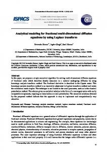
Figure 1. A triangular region Ω (left) transformed into an equivalence class of welding maps φ (right). Four members of the equivalence class are shown. Four segments of ∂Ω are drawn with differing linestyles to highlight their corresponding segment on each of the welding maps.

Möbius group P SL2 (R) of conformal self-maps of the unit disk. Both Φ+ , Φ− extend continuously to the boundary S 1 , and their composition Φ−1 − ◦ Φ+ , restricted to the boundary, 1 1 is a map Ψ : S → S . A remarkable result (see [2], for example) is that this result is almost an isomorphism: the space of shapes, modulo translation and scale, is isomorphic to the group Diff (S 1 ), modulo conformal self-maps of the disk. This provides an elegant way of making the space of shapes into a metric space: we take an element of the coset space P SL2 (R)\Diff (S 1 ), i.e. an equivalence class of diffeomorphisms of the circle, as a representation of a shape. This space is known as the universal Teichm¨ uller space and was initially studied in the context of Riemann surfaces [2, 7] it also arises in string theory [3, 14]. In [16] elements of P SL2 (R)\Diff (S 1 ) are called “fingerprints”; in the mathematical literature, elements of the broader class of quasisymmetric homeomorphisms of S 1 are commonly known as “welding maps” and each has an associated quasicircle. We illustrate an example of a equivalence class of welding maps in Figure 1 for a simple shape. 1.2. The Weil-Peterson Riemannian metric. The Lie algebra to P SL2 (R)\Diff (S 1 ) is the space fields on the circle modulo the subspace spanned by 1, cos and sin. If P of vector inθ ∂ is a real-valued vector field on the circle, the Weil-Peterson norm v(θ) = ∞ a e n n=−∞ ∂θ is ∞

X 1

(3/2) 2 (1/2) 2 2 3 2 (1) kvkW P = (n − n)|an | =

v

− v

2 n=2

where k·k denotes the L2 norm.

1

This may be rewritten as kvk2W P = hLv, vi

1This formula, while explicit, is troublesome in numerical computations; the boundary values of conformal

maps have so much high-frequency content, even for curves with real-analytic boundaries, that the number of Fourier coefficients required for for an accurate global representation is prohibitive.

COMPUTATION OF WEIL-PETERSON GEODESICS

3

for the positive semidefinite, self-adjoint operator L = −H(∂ 3 − ∂)

(2)

where H is the Hilbert transform. Note that L has a kernel which is exactly the span of and sin. As mentioned above, the corresponding vector fields in the span of 1, cos ∂ ∂ ∂ sin θ ∂θ , cos θ ∂θ , ∂θ are infinitesimal Möbius maps; i.e. they span the Lie algebra psl2 (R) of the M¨ obius group P SL2 (R). Hence, our norm is indeed a norm on the quotient space. By right-translations we extend this norm to the entire space; that is, if φ(θ, t) ≡ φt (θ) is a curve in P SL2 (R)\Diff (S 1 ), then any any time t we pull back the velocity φ˙ t under the derivative of right translation to obtain vt (θ) = φ˙ t ◦ φ−1 t The length of a curve φ : [0, 1] × S 1 → S 1 in Diff (S 1 ) is obtained by integrating Z 1 kφ˙ t ◦ φ−1 L[φ] = t kW P dt 0

The resulting Riemannian metric is known as the Weil-Peterson metric. The classical definition was in terms of Beltrami differentials of quasiconformal self-maps of the hyperbolic plane and was originally studied in the context of Teichm¨ uller theory. The formulation we present here occurs naturally in string theory where it was discovered as the unique Kähler metric on P SL2 (R)\Diff (S 1 ) [15]. See [14] for a thorough discussion of how this Kähler metric agrees with the classical WP metric. It is a fact from variational calculus that minimizing length is equivalent to minimizing energy: the path of least energy is a constant-speed parametrization of the path of least length. Thus given a pair of points h0 , h1 ∈ Diff (S 1 ) we find the geodesic by finding the path φ of minimum energy Z 1 2 (3) kφ˙ s ◦ φ−1 E[φ] = s kW P ds, φ0 = h0 , φ1 = h1 0

Finding this minimizing φ is the problem we are concerned with. It is a fact that all sectional curvatures of the WP metric are negative [19], which in finite dimensions would imply that minimizing geodesics are unique. While the existence and uniqueness of minimizing geodesics is a subtle issue in infinite dimensions, both questions were recently answered in the affirmative in [6]: Any two points in P SL2 (R)\Diff (S 1 ) are joined by a unique geodesic, and further, solutions to the geodesic equation exist for all time and the resulting welding maps are Sobolev H s for any s < 3/2, where the inequality is sharp. It is an essential fact that the WP metric we have described here is, by construction, right-invariant. That is, given any h0 , h1 , define the map g by h0 = g ◦ h1 and let φ(θ, s) be the shortest path from g to the identity. Right-invariance of the metric means that the length of φ(θ, s) is the same as length of φ(h1 (θ), s), which immediately implies that the shortest path from h0 to h1 is in fact φ(h1 (θ), s). Hence, computing geodesics between two welding maps reduces to the case where one of the maps is the identity. Therefore in what follows we consider only paths ending at the identity. 2. The Discrete Problem We now discretize the problem (3) in the case where h0 : S 1 → S 1 is an arbitrary welding map and h1 is the identity map. This is a boundary-value minimization problem: find vs = φ˙ s ◦ φ−1 subject to initial and terminal conditions φ0 = h0 and φ1 = Id such s

4

FEISZLI AND NARAYAN

R that kvs k2W P ds is minimized. Becuase we eventually adopt a Lagrangian framework we introduce q ≡ φ, and given a velocity field v then Z t v(ξ, q(ξ, x))dξ q(t, x) = q(0, x) + 0

for all 0 ≤ t ≤ 1. We track M particles on the range of q as they evolve in t. For some fixed xm on S 1 , q(t, xm ) are the locations of these particles. The velocity field v(t, ·) at the locations q(t, xm ) is likewise stored. We store these velocity field values and recover the particle positions q(t, xm ) by integrating rather than directly storing the particle positions. In the next subsection we will describe how we compute the W P norm at each time. We delay discretizing the t variable until Section 3.

2.1. Computing the WP Norm. We first consider the problem of computing the norm of a vector field on S 1 . Subsequent sections will consider computation of path energy and its gradient to find geodesics. Our discretization provides us with information about the velocity field only at a discrete set of points. Our first task is to interpolate this velocity field to a field defined on all of S 1 and then compute the norm of this lift. The computation proceeds in 3 steps. We first collect some standard results which let us do this when the metric has no kernel. Next we compute the optimal interpolant and its norm when the metric has a kernel; this is done by projecting the interpolation data onto the orthogonal complement of the kernel and computing the norm of the lift. Finally, we generalize the problem to allow an arbitrary basis for the interpolating functions; this allows for more flexibility in the implementation and also suggests a more stable method of computation, which we detail later. 2.1.1. Lifting the velocity field into the orthogonal complement of the kernel. We need to extend a vector field defined on a finite subset of S 1 to a vector field on all of S 1 . Here we describe a method for finding the smoothest possible extension using Green’s functions for the operator L. In this section we consider only vector fields orthogonal to the kernel; we extend to more general cases next. Consider the space of all vector fields on S 1 , and a subspace on which k · kW P is a proper norm: V = {v : kvkW P < ∞}, Ve = {v ∈ V : v ⊥ kerV L}, where, explicitly, kerV L = span{1, sin, cos}. Let LM be the M -manifold of configurations of M points q1 < q2 < ... < qM on the unit circle and write Q = {q1 , q2 , ..., qM }. The tangent space TQ LM is the M -dimensional space of vector fields v = (v1 , v2 , ..., vM ) supported on the set Q. We consider all possible extensions of v to vector fields defined on the entire circle, and induce a norm on TQ LM by (4)

kvkW P (Q) ≡ inf {ke v kW P : ve(qm ) = vm , 1 ≤ m ≤ M }

Conversely, given the basepoint Q, consider the evaluation map taking a global vector field ve, defined on all of S 1 , to TQ LM by ve → (e v (q1 ), ve(q2 ), ..., ve(qM ))

This map induces a splitting of any ve into two components. The set of vector fields for which ve(qm ) = 0 for all 1 ≤ m ≤ M is the vertical subspace (of the Lie algebra of Diff (S 1 ): the set of smooth vector fields on S 1 ), and its W P -orthogonal complement is the horizontal subspace; the minimizing extension in (4) of v ∈ TQ LM is known as a horizontal lift.


5

As the next proposition shows, the horizontal subspace is an M -dimensional subspace spanned by translates of Green’s function for the operator L = −H(∂ 3 − ∂). This Green’s function is known explicitly, see [9]: ∞ X cos(nθ) 3 G(θ) = 2 = (1 − cos θ) log [2(1 − cos θ)] + cos θ − 1 3 (n − n) 2 n=2

The following results are standard facts which may be proven using the reproducing kernel ∂ property of Green’s function and the fact that the vector fields G(θ − qm ) ∂θ lie in the horizontal subspace. Proposition 1 (Computing Horizontal lifts). (1) The set of vector fields

∂ G(θ − qm ) ∂θ

M

m=1

is a basis for the component of the horizontal subspace in Ve . (2) The horizontal lift on Ve of the tangent vector (v1 , ..., vM ) ∈ TQ LM is the vector field ∂ ve(θ) ∂θ for ve(θ) =

M X

G(θ − qi )pi

where

pi =

i=1

G−1 ij vj

j=1

and Gij is the positive definite symmetric matrix (5)

M X

Gij = hG(· − qi ), G(· − qj )iW P = G(qi − qj ) Further, ke v k2W P =

X

G−1 ij vi vj

i,j

2.1.2. Lifting the velocity field. Now we extend these results to compute horizontal lifts which take into account the kernel. Lemma 1. Let G be an M ×M positive matrix, B an M ×K full-rank matrix with K < M . Then given some v ∈ RM , the projection of v onto the G−1 -orthogonal complement of the kernel of B T is given by . PGB v = (I − B(B T G−1 B)−1 B T G−1 )v In our case B is an M × 3 matrix containing point evaluations of a basis for the threedimensinal kernel of the W P norm. Once we have subtracted out the contribution of the kernel, we may compute the lift and its norm. The next result is a corollary of section 2.1.1 and the previous lemma. Corollary 1. Fix Q and let the matrix G be as in Proposition 1. For any v ∈ TQ LM , kvk2W P (Q) = v T G−1 PGB v

(6)

Further, the horizontal lift ve of v to V is given by ve =

3 X j=1

wj bj (·) +

M X j=1

G−1 PGB v

j

G(· − qj )

6

FEISZLI AND NARAYAN

3 Ve interpolant, kvkW P = 14.94 V interpolant, kvkW P = 1.71 Data

2

Ve interpolant, kvkW P = 9.58 V interpolant, kvkW P = 4.35 Data

2

1

e v

e v

1

0 0 −1 0

1

2

3 θ

4

5

6

0

1

2

3 θ

4

5

6

Figure 2. Interpolation procedures from (a) Proposition 1 on the quotient space Ve , and from (b) Corollary 1 on V . Left: the data is taken from the function v(θ) = sin(2θ)+cos(θ) on 15 randomly distributed θ locations. Right: the data is taken as Gaussian random variable perturbations of function values from v(θ) = sin(2θ) on 15 randomly distributed θ locations.

where w = (B T G−1 B)−1 B T G−1 v and {bj }3j=1 is the basis for kerV L used to construct B: Bm,k = bk (qm ). Remark. The vector p = G−1 PGB v contains what are known as the momenta coefficients. Similarly,we call w the kernel coefficients. The interpolant produced from Corollary 1 is notably different than the horizontal lift from the quotient space in Proposition 1. This is exemplified in Figure 2. Up to this point, we have taken Green’s functions centered at the interpolation nodes as as the basis for our interpolating space. As discussed, this produces the norm-minimal lift. While this optimality is nice, and is in fact what our current implementation ultimately uses, one might wish to choose a different space of interpolating functions. For example, the first N complex exponentials, or a wavelet basis adapted to the problem might be reasonable choices. We address this now; it is only a small modification to the calculations above and admits a stable solution which we present later. Let VeN be any N -dimensional subspace of Ve such that the interpolation problem for data collocated at Q is unisolvent. If F = {fn (·)} is a basis of VeN , define the M × N matrix λF to have entries (λF )m,n = hfn , G(· − qm )iW P = fn (qm )

Let GF be the N × N Gram matrix for the fn : (GF )m,n = hfm , fn iW P For v ∈ RM interpolation data on Q, define VeN (v) as the subset of functions from VeN ⊕kerV L that interpolate to v. Then define kvk2W P (Q),Ve = N

min

v∈VeN ⊕kerV L

kvk2W P


7

The results from the previous section may be rephrased by replacing G ← GF where T e GF = λF G−1 F λF . Since VN is total for interpolation, then GF is invertible. One finds that all formulas carry over essentially up to change-of-basis. This, then, is our most general result for computing lifts, which we state in terms of an operator LF . Proposition 2. In the notation above, set B LF = G−1 F PGF

Then kvk2W P (Q),Ve = v T LF v

(7)

N

=: v T p. The reconstruction ve ∈ VeN ⊕ kerV L is given by ve =

where

N X

cn fn +

n=1

w = B T G−1 F B

(8a)

3 X

wj bj

j=1

−1

B T G−1 F v

T −1 c = G−1 F λF GF (v − Bw).

(8b)

Note that unlike the result of Corollary 1, the momenta p ≡ LF v are no longer the reconstruction coefficients for the lift unless VeN is the span of Green’s functions centered at Q. In any case, LF is a symmetric, rank M − 3, positive semidefinite matrix. Whether using Green’s function interpolation or another basis, using (7) and (8) to compute either the norm or any coefficients can be problematic. The matrices in the explicit formula given can easily be ill-conditioned, depending on F and Q. We do not directly solve this issue here, but instead we reformulate the problem in a format that we observe is more robust with respect to numerical precision issues than the above formulas. This is done in Section 3. 2.2. Path energy and its gradient. Computing the length and energy of a path is relatively straightforward given the work in the previous section. If v t is a vector of velocity evaluations at time g, we have Z 1 Z 1 2 E= ke v kW P dt v t LtF v t dt, 0

LtF

0 qt.

where is the metric on the particle positions We compute the gradient of energy for our discrete boundary-value problem in two steps. We first compute the gradient for the unconstrained problem; i.e. we compute an update to the velocity field which simply makes the energy smaller, ignoring the boundary conditions at times 0 and 1. We then project this update onto the space of admissible updates; i.e. those updates which preserve the boundary conditions. This two-step trick is equivalent to simply taking the first variation of energy for the fixed-endpoint problem, but is considerably simpler to derive, carries little performance penalty, and makes it possible to alter the space of admissible updates at run-time easily. Since we have yet to discretize the temporal variable, we wait to compute the uncontrained gradient until Section 3. For now we concentrate on the projection into the space of admissible updates.

8

FEISZLI AND NARAYAN

Define the energy of a velocity field as above. Now consider two manifolds of velocity fields. N contains all velocity fields defined on M particles at each time, and M ⊂ N contains those which respect the boundary-value conditions. N = {e v : {1, ..., M } × [0, 1] → R} Z M = V ∈ N qm (1) = qm (0) +

0

1

ve(ξ, qm (ξ))dξ

We defined the energy E : N → R as a function on N , and in the next section we will describe the computation of its gradient ∇E on N . With this gradient in hand, we obtain the direction of steepest ascent as a projection of ∇E (a coordinate-dependent quantity) onto the manifold M by projection in the following metric. Let P be the space of smooth paths on P SL2 (R)\Diff (S 1 ). Let q(t, x, s) = qt;s (x) be (a representative of) a smooth curve in P. Variable x is position on S 1 , t parametrizes a path for given s, and s parametrizes the curve of paths. We define the velocity vt;s along the path by Z t q(t, x, s) = q(0, x, s) + vξ;s (q(ξ, x, s))dξ 0

I.e. for fixed s the path of a particle q(·, x, s) is obtained by integrating the Eulerian vector field vt,s in t. To construct a metric we place a norm on the Lie algebra and extend to the whole manifold by right translations. We write ∂ q˙ ◦ q −1 t;s (9) wt;s = ∂s and introduce the norm Z 1 2 (10) kwkP ≡ kwt;s k2W P dt 0

We take the metric on path space to be the Riemannian metric induced by the norm ∂ q, k · kP . However, we wish to work on the manifolds N and M. With q = q(t, x, s), q˙ = ∂t ∂ 0 and q = ∂x q, we have −1 ∂ q˙ ◦ q −1 t;r ∂q ∂ q˙ −1 0 −1 + (q˙ ◦ q )t;r (x) = ◦q ∂r ∂s ∂s t;r t;r −1 ∂q ∂v 0 = + vt;r ∂s t;r ∂s t;r 0 ∂v ∂q 0 = − vt;r q −1 t;r ◦ q −1 ∂s t;r ∂s Direct computation yields

Therefore

Z t ∂qs ∂ ∂ (t, x) = q(0, x, s) + vξ;s (q(ξ, x, s))dξ ∂s ∂s ∂s 0 Z t ∂ = vξ;s (q(ξ, x, s))dξ 0 ∂s ∂ q˙ ◦ q −1 ∂r

t;r

∂v (x) = Y , ∂s


where the linear operator Y is given by (11)

Y(t, x, s) = Id − v 0 q −1

0

Z

9

t

(·)ξ dξ

0

This operator Y gives a mapping from velocity field updates (i.e. tangent vectors to N or M) to tangent vectors ∂q ∂s to P. Hence our metric on path space immediately induces a metric on N and the submanifold M. We make our projection of the update to the velocity field with respect to this metric. 3. Computations We now address the more practical issues of implementation of the methods described. We first formulate computation of the W P norm as a classical numerical linear algebra problem. Following this is presentation of the temporal discretization; having discretized both the temporal and S 1 variables, we can compute the unconstrained coordinate gradient of the energy. Finally, the submanifold projection for gradient updates is discretized. 3.1. The WP norm. It is not necessary to explicitly form the metric matrix LF as defined in Proposition 2. We can accomplish the same task in a more stable manner using some established numerical linear algebra results. Given an M × N matrix A, A† denotes its Moore-Penrose pseudoinverse. For any b ∈ RN , the vector A† b is the minimum-norm, least squares solution to Ax = b. Here, both minimum-norm and least squares refer to the `2 (Euclidean) metric on x and b, respectively. For computation of the W P norm, we develop the ideas for a general subspace VN of V and then specialize to the minimal-norm lift over all V using Green’s functions. Our goal is the interpolation of data v ∈ RM collocated at Q with an element from VeN ⊕ kerV L; thsu we are essentially trying to find the minimal norm solution to c λF B (12) =: Ax = v, w

where the norm over the coefficients c is given by the positive (Gram) matrix GF and that over the kernel coefficients w is zero. Again we assume that VeN is total for interpolation on Q, implying that Ax = v has at least one solution. Let GF0 be a block diagonal matrix with GF in the upper-left block and a 3 × 3 zero matrix in the lower-right block. It is easy to show that ker(B) is trivial so long as M ≥ 3. This implies that ker(GF0 ) ∩ ker(A) is trivial and therefore the minimum norm solution to (12) is unique [5]. This is an easy way to show uniqueness of the lift defined in (4). Restating (12), we are trying to solve the minimization problem: (13)

minimize

kRxk2

subject to

Ax = v,

where R is any matrix square root of GF0 . (I.e. RT R = GF0 .) One of the standard tools for solving least squares equality constrained problems is the generalized singular value decomposition (GSVD) [11]. Since A and G(F )0 have the same number of columns, the GSVD matrix decomposition of (A, R) is given by (14a)

A = U CX −1

(14b)

R = V SX −1 ,

where U and V are orthogonal matrices, X is invertible, and C and S each have only one non-vanishing diagonal with non-negative entries and satisfy C T C + S T S = I. (Here, V

10

FEISZLI AND NARAYAN

denotes a matrix in the GSVD decomposition, and not a linear subspace.) The solution to (13) is given by c (15) x= = XC † U T v, w

The above matrix mapping v to x is a weighted pseudoinverse of A with respect to R. The momenta are p = U C †T X T GF0 x = LF v. Our experience is that this is a much more stable way to compute momenta than the explicit matrix relations used to define LF . Note that since C † is a matrix with only one non-vanishing diagonal, applications of C † can be accomplished with a simple vector-vector multiply. The norm is kvkW P (Q),VeN = cT GF c = vT p. For the horizontal lift from the whole space V , we need only take the space VeN to be the M -dimensional space of Green’s functions centered at the qm . Notable simplifications in this case are that (a) GF = G, with G being the Gram matrix of Green’s functions (5) and (b) the momentum and basis coefficients coincide: p = c. 3.2. Temporal discretization. Since flow along the geodesic is reversible, we use a quadrature method that is symmetric with respect to the endpoints. We rewrite the flow of particles in an equivalent form Z t Z 1 1 1 (16) qm (0) + ve(ξ, qm (ξ))dξ + qm (1) − ve(ξ, qm (ξ))dξ qm (t) = 2 2 0 t

Now choose T ordered points st on (0, 1); let qt and vt denote the M particle positions and velocities, respectively, at those times. The endpoint particle positions q0 and qT +1 given. Let ht denote the quadrature weight associated with data at time st so that Rare PT 1 t t t=1 h f (s ). 0 f (s)ds ' Following (16) we use the quadrature rule to to integrate particle positions forward from q0 to qt , and backwards from qT +1 to qt , and average the result. For example if the representation is piecewise-linear, then the symmetric velocity-to-particle map is ! ! t−1 T t t X X 1 h 1 h qt = (17) q0 + hr vr + vt + qT +1 − hr vr − vt , t≥1 2 2 2 2 r=1

r=t+1

The scheme described above expresses particle positions qt linearly with the velocity field values vr . Collect all the velocity evaluations into a matrix V , of size M × T ; do the same for the particle positions in a matrix Q. Then regardless of the choice of linear temporal quadrature rule, there exists a T × T matrix Z such that 1 (18) Q= Q0 + QT +1 + V Z, 2 0 T +1 where Q and Q are matrices with the known vectors q0 and qT +1 repeated. The entries of the matrix Z depends on the choice of temporal representation and quadrature. For the piecewise-linear choice, it has entries Zr,t = 21 cr,t hr , where   0, r = t, 1, r < t, (19) cr,t =  −1, r > t. R1 In order to evaluate the energy 0 kvs k2W P ds, we build the quadrature factor ht into the norm at each point in time. This can be accomplished by simply replacing G(F ) by ht G(F )


11

at each point in time. Therefore (20)

E=

T X t=1

kvt k2W P (Q),Ve = N

T X

(vt )T LF vt

t=1

where LF is time-varying, depending explicitly on qt , the particle locations at time st , and also depending proportionally on ht . To keep the presentation simple we have described use of a piecewise-linear quadrature. In practice we find it is sometimes more efficient to use a Legendre-Gauss-Lobatto quadrature rule for t ∈ [0, 1], which enables a high-order polynomial representation for each particle’s velocity field. When to use a high-order representation versus a piecewise linear representation depends on whether one expects large t-derivatives in the velocity field. B 3.3. The gradient of the WP norm. At some time st , we have seen that if LF = G−1 F PG F then formula (20) defines the norm, and to minimize we must compute variations of this with respect to velocity evaluations. Since the particle positions are influenced by (18), the matrices LF and therefore the energy change in nontrivial ways when we vary vt . To simplify the procedure, we first fix t and consider only variations in kvt kW P (Q) with respect to vr for r = 1, . . . , T . Direct variation of the quadratic form yields ∂ ∂ t 2 t T t T t kv k = 2δ (v ) L + (v ) L t,r F F v W P (Q),VeN ∂vr ∂vr ∂ t T t T (21) LF vt = 2δt,r (p ) + (v ) ∂vr

where δi,j is the Kronecker delta. The metric LF and its components GF and PGBF are generated from qt , depending on vt . Using simple properties of matrix algebra, a straightforward but messy computation yields a formula for the variation of the objective with respect to the particle positions. Lemma 2. Let λ(F 0 ) be the M × N matrix with entries λ(F 0 )m,n = fn0 (qm ) and B 0 be the 0 M × 3 matrix with entries Bm,j = b0j (qm ). For two matrices C and D of the same size, C ◦ D denotes the elementwise product. Then (22)

t ∂ t 2 0 −1 T t 0 t T kv k = −2 p ◦ λ(F )G(F ) λ(F ) p + B w . e W P (Q),VN ∂qt

In particular, if F is a basis of Green’s functions centered at Q, then (23)

T ∂ kvt k2W P (Q) = −2 pt ◦ ve0 (qt ) , t ∂q

where ve0 is the derivative of the horizontal lift from V .

The salient result of Lemma 2 is that computing variations of the W P norm with respect to particles is quite easy once we have the momentum coefficients p and kernel coefficients w in hand from the GSVD. The only additionaly difficulty could come in computing entries for λ(F 0 ). In all the straightforward choices for F we make, it is not a deterrent.

12

FEISZLI AND NARAYAN

3.4. The gradient of energy. With the gradient of the W P norm computed, computing the energy is now straightforward. Combining (18), (21), and (22), we have X T 1 ∂E t T (24) Zt,r pt ◦ λ(F 0 )G(F )−1 λ(F )T pt + B 0 wt = (p ) − t 2 ∂v r

where again we recall that the momenta coefficients pt already have the scaling factor ht included. Although the above equation is an exact formula for the gradient, updating velocity fields P with these values will not respect the endpoint constraint q1 = q0 + t ht vt , and so we project into the space of admissible updates. The discrete versions of the manifolds presented in Section 2.2 can be defined as follows: N = {v : [1, ..., M ] × [1, ..., T ] → R} ) ( X 1 ht vt M = v ∈ N q = q0 + t P t 1 0 Since the condition q = q + t ht v is linear, we may write it as q1 − q0 = Av

for some constraint matrix A. We see that M is an implicit submanifold of N : it is the q1 − q0 level set of the function Av. By the implicit function theorem, the tangent space to M at any point is equal to the nullspace of the differential DA, and we have simply [DA] = A. That is, the admissible updates to a given velocity field V are exactly those vectors v in the nullspace of A. In order to perform the appropriate projection onto the nullspace of A, we place our update along a curve on the space of paths P and apply the norm induced by the metric (9) and (10). We then seek a discretization of the semidefinite operator Y † LY given by (11) and (2), where Y † is the L2 adjoint of Y. At a fixed value of st , we have already approximated L with LF depnding on qt . Therefore R st we concentrate on Y: the integral 0 (·)ξ dξ is approximated by the t-th column of Z. Let e = Z T ⊗ IM , where IM is the M × M identity matrix; then q = Zv. e The factor v 0 (q) can Z 0 t 0 t 0 t be computed at each t via v (q ) = λ(F )c + B w . We collect these factors into a diagonal M T × M T matrix W with the t-th block diagonal entry (W t )j,j = v 0 (qjt )(q −1 )0 (qjt ). The ∂ result then is the modified metric on updates ∂v E: (25)

fF = (I − W Z) e T LF (I − W Z). e L

e is our approximation to the operator Y. We use this metric I.e., the matrix Y := I − W Z both to form the natural gradient and to orthogonally project into the nullspace of the constraint matrix A. 4. Algorithm and Results With all the necessary derivations complete, a summary of the minimization algorithm is presented in Algorithm Listing 1. One detail we have not yet addressed is a method for computing welding maps – i.e. for determining φ given a discrete collection of ordered samples on ∂Ω. A few standard methods exist for numerically computing conformal welds [4, 10, 17, 18], and we settle upon the Zipper algorithm [12]; specifically we use the (simplest) ‘geodesic’ version. We use the Zipper algorithm to (a) construct a representation of a conformal weld given discrete samples on the shape boundary ∂Ω, (b) ‘interpolate’ the


13

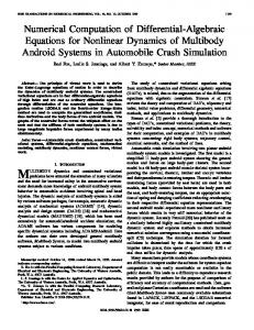
welding map to any starting particle locations q0 ,qT +1 of our choosing, and (c) ‘invert’ the weld: compute a representation of a simple closed curve from discrete samples of a homeomorphism of S 1 . There are other possibilities for accomplishing these conformal welding tasks [16]. Algorithm 1 A simple gradient descent algorithm for optimization. Input: Initial and final particle positions q0 and qT +1 Initialize: vt = qT +1 − q0 for all t while Not converged do Compute norm, momenta, and kernel coefficients from (15) Compute standard unconstrained gradient ∇E from (24) and (22) g n from (11) and (25). Form projected natural gradient ∇E g Find ε such that E(V − ε∇E n ) < E(V ) g n , update particles using (18) Update V ← V − ε∇E end while Output: Velocity field V Our stopping criterion for the optimization iteration is defined by monitoring the relative objective decrease at each step in tandem with the Euclidean vector 2-norm of the projected natural gradient (normalized with respect to the size of the vector). At convergence, the former is less than 10−8 and the latter is less than 10−6 . One necessary measure of convergence is constancy of the W P norm along the path. For all the results we show, the relative variation measure (maxt kvt k2W P (Q) )/(mint kvt k2W P (Q) )− 1 is no larger than 10−3 and is usually O(10−6 ). In all the tests we use 150 particles. The full set of particles is obtained by computing 50 uniformly distributed particle samples on the ranges of the two welding maps φ0 and φ1 , and 50 on the domain of the welding maps, and then taking the union of the sets. This encourages inclusion of resolvable features from both the interior and exterior of the welds in the computation. For the temporal discretization, we have found that using a high-order Gauss-Lobatto quadrature rule works very well for welding maps whose derivatives are not large. When the welding maps exhibit high frequency content (a result of e.g. protrusions in the shape), then a standard piecewise linear choice works well. In this latter case we use 150 equispaced points in the time variable. 4.1. Zero-distance welds. As a first test we compute the energies of the paths connecting welding maps in the same equivalence class (which are expected to vanish). The welding maps are the maps φi in Figure 1. In Table 3 we show the computed energy at convergence. The shown near-vanishing energies confirms validity of the computation. 4.2. Path length vs aspect ratio. Let ψtr be a geodesic where ψ0r is the welding map for an ellipse of aspect ratio r, and ψ1r is the identity. In Figure 4 we show results of simulations for path lengths L[ψ r ] versus aspect ratio r ranging from 1 to 5. The results suggest that the asymptotic relation is approximately linear, and these results match those obtained in [8] very well.

14

FEISZLI AND NARAYAN

2π

E ↔ φ2 7.530 × 10−12 ↔ φ3 1.249 × 10−9 ↔ φ4 2.853 × 10−9 ↔ φ3 1.729 × 10−8 ↔ φ4 6.633 × 10−8 ↔ φ4 2.069 × 10−10

φ(t, θ)

φ1 φ1 φ1 φ2 φ2 φ3

t = 0, 1 t = 0.2, 0.4, 0.6, 0.8

0

0

θ

2π

Path length L

Figure 3. Left: computed path energies between welding maps in the same equivalence class shown in Figure 1. The near-zero value of the energies verifies that the computed paths are accurate geodesics. Right: evolution snapshots of φ(t, θ) at t = 0, 0.2, 0.4, . . . , 1 where φ(0, ·) = φ3 and φ(0, ·) = φ4 .

∼ 0.69

3 2 1

Minimization algorithm

t = 0, 1 0