BIT 2003, Vol. **, No. *, pp. 00*–00*
0006-3835/00/4004-0001 $15.00 c Swets & Zeitlinger °
Numerical evaluation of the Evans function by Magnus integration∗ NAIRO D. APARICIO1 , SIMON J.A. MALHAM2 and MARCEL OLIVER3
October 21st, 2004 1
Department of Mathematical Sciences, Oxford Brookes University, Wheatley OX33 1HX, UK. email:
[email protected] 2 Department of Mathematics, Heriot-Watt University, Edinburgh EH14 4AS, UK. email:
[email protected]
3
School of Engineering and Science, International University Bremen, 28759 Bremen, Germany. email:
[email protected]
Abstract. We use Magnus methods to compute the Evans function for spectral problems as arise when determining the linear stability of travelling wave solutions to reactiondiffusion and related partial differential equations. In a typical application scenario, we need to repeatedly sample the solution to a system of linear non-autonomous ordinary differential equations for different values of one or more parameters as we detect and locate the zeros of the Evans function in the right half of the complex plane. In this situation, a substantial portion of the computational effort—the numerical evaluation of the iterated integrals which appear in the Magnus series—can be performed independent of the parameters and hence needs to be done only once. More importantly, for any given tolerance Magnus integrators possess lower bounds on the step size which are uniform across large regions of parameter space and which can be estimated a priori. We demonstrate, analytically as well as through numerical experiment, that these features render Magnus integrators extremely robust and, depending on the regime of interest, efficient in comparison with standard ODE solvers. AMS subject classification: 65F20. Key words: Neumann expansion, Magnus expansion, Evans function.
1
Introduction
We seek efficient numerical methods for solving a low-dimensional system of linear non-autonomous ordinary differential equations many times for different values of one or more parameters that appear in the equation. More specifically, we consider (1.1) ∗ Received
Y˙ = A(t, λ) Y ,
Y (0) = Y0 ,
October 2003. Communicated by ****.
2
N.D. Aparicio, S.J.A. Malham and M. Oliver
where Y (t) ∈ Cn , and A is a time-dependent n × n matrix that depends linearly on a parameter vector λ ∈ Cp , (1.2)
A(t, λ) = A0 (t) +
p X
λk Ak (t) .
k=1
In the following, we will always take p 6 2. Extensions to a larger number of parameters are straightforward in principle, but the computational complexity of our approach scales unfavourably with p, so that larger values are of no practical interest. Differential equations of this type arise, in particular, when evaluating the Evans function—the discriminant of a spectral problem that is associated with the linear stability of systems of reaction-diffusion partial differential equations. In the most direct approach, we could integrate the system from 0 to some final time T for each value of λ we wish to sample. If we need to sample only in a small neighbourhood of parameter space, efficiency could be increased by using continuity arguments. Often however, we need to cover a wide range of parameter values. Worse, the behaviour of the solution, e.g. the stiffness of the problem, is not known in advance and may change significantly as λ varies. We therefore try to formulate the problem in a way that a substantial portion of the computational effort can be done independent of the parameters. For a Runge–Kutta scheme, for example, the Ak (t) can be evaluated and the stages can be combined in a precomputation step, so that each Runge–Kutta time step can be written as the multiplication of a vector with a matrix-valued polynomial in λ. Relatively more work can be put into the precomputation step when using methods based on Neumann or Magnus expansions, as both involve nested commutators and time integrals which can be evaluated independent of λ. On the other hand, Magnus integration involves a relatively expensive computation of a matrix exponential at each time step. We thus ask whether Neumann or Magnus integrators allow significantly longer time steps than Runge–Kutta, so that such additional expenses pay off. For Neumann integrators the answer is clearly negative. In fact, Runge–Kutta methods can be interpreted as truncated Neumann expansions with a particular choice of quadrature; precomputing these integrals to higher order than necessary does not significantly reduce error. Nonetheless, the Neumann series is conceptually important, and the derivation of the Magnus series can be easily implemented on a computer algebra system by taking the formal logarithm of the Neumann series. Magnus integrators, on the other hand, are well known for their superior stability and applicability to solving stiff problems [19, 20]. The main point of this paper is to demonstrate, by computing leading order error terms as well as by numerical examples, that their behaviour is uniform and predictable, in the sense that error control can be made part of the precomputation step, over bounded regions of parameter space. In particular, it is easy to find situations where Runge–Kutta methods may perform arbitrarily poorly in comparison. Our work generalizes a scheme proposed by Moan [30] for Sturm–Liouville
Numerical evaluation of the Evans function
3
problems which was recently extended by J´odar and Marletta [26] and Greenberg and Marletta [15] to non-selfadjoint Sturm–Liouville problems. We consider the eigenvalue problem for arbitrary elliptic operators in one-dimension, providing: 1. a treatment of the multi-parameter case (useful, for example, for determining linear stability of planar waves and pulses); 2. formal error analysis which shows that errors are nearly uniform over large regions in parameter space, and opens up the possibility for a priori stepsize control and adaptivity; 3. detailed analysis of the nearly autonomous regime; 4. cost comparison with classical precomputation schemes. Numerical schemes based on the Magnus expansion received a lot of attention due to their preservation of Lie group symmetries—see Iserles and Nørsett [24], Munthe-Kaas and Owren [33], and references cited therein. More generally, Neumann and Magnus methods have been applied in spectral theory, Hamiltonian systems, symplectic and unitary integration, control theory, stochastic systems, and quantum chemistry; see Blanes et al. [8] for an extensive list of applications. For recent progress on high order Magnus schemes see Iserles and Nørsett [24], Munthe-Kaas and Owren [33], and Blanes, Casas and Ros [7]. The numerical solution of Sturm–Liouville problems is usually done by finite differencing, variational methods such as finite elements, shooting via scaled Pr¨ ufer methods or Pruess-type methods (see, for example, Pryce [36]). The first two methods only deliver a finite spectrum. Scaled Pr¨ ufer methods can suffer from initial value stiffness problems, though there are methods that can help with this—none better than the Magnus methods we advocate here. Pruess methods approximate the coefficients of the problem by piece-wise constant approximations, solving the problem analytically on the piece-wise constant intervals. They circumvent the problems mentioned thus far but are only second order unless Richardson extrapolation approximations or other modifications are made. Magnus methods are the natural extension of these ideas—see Moan [30], J´odar and Marletta [26], Chanane [9], and Greenberg and Marletta [15], who also provide comparisons with traditional approaches. The Evans function is now a standard tool in non-selfadjoint spectral theory for calculating unstable eigenvalues of linear differential operators. Recent applications have included the detection of instabilities analytically and numerically in nerve impulses by Alexander, Gardner, and Jones [1], high activation energy combustion by Terman [40], solitary waves by Pego and Weinstein [35], multi-bump pulses by Sandstede [38], boundary layer interactions with compliant surfaces by Allen and Bridges [2] and travelling wave solutions to neural field equations by Coombes and Owen [11]. Our paper is organized as follows. In Section 2 we review the Neumann and Magnus series solutions to systems of linear ordinary differential equations. In Section 3 we set up the precomputation procedure for both Neumann and Magnus integrators. We explicitly analyze and compare the local truncation errors
4
N.D. Aparicio, S.J.A. Malham and M. Oliver
of each of the methods in Section 4 and contrast their relative efficiencies and accuracies. We perform some numerical experiments in Section 5 confirming these results. Section 6 introduces the Evans function and sets up our numerical method in this context. We demonstrate the practical advantages of the Magnus method by calculating the onset of the well-known pulsating instability for a system of reaction-diffusion equations modelling autocatalysis. Lastly, in Section 7, we outline extensions and refinements of our method for future development. 2
Neumann and Magnus expansions
Disregarding any parameter dependence for the moment, consider the initial value problem in C ∞ (R; Cn×n ) for the flow-map or fundamental matrix S(t) of (1.1), S˙ = A(t) S ,
(2.1)
S(0) = I ,
where the matrix of coefficients A(t) ∈ C ∞ (R; Cn×n ). If A(t) belongs to an Abelian Lie algebra, the solution is Z t A(τ ) dτ . (2.2) S(t) = exp 0
For the general case, there are several fundamental solution expansions. Here we focus on Neumann and Magnus series, though the Fer expansion is another important example (see Iserles, Munthe-Kaas, Nørsett and Zanna [23], for example). The integral form of the initial value problem (2.1) is (2.3)
S(t) −
Z
t
A(τ ) S(τ ) dτ = I 0
or, more abstractly, (2.4)
(I − K) ◦ S = I ,
where K is the integral operator defined by Z t ¡ ¢ (2.5) K ◦ F (t) ≡ A(τ ) F (τ ) dτ , 0
for any F ∈ L1loc (R; Cn×n ). We can formally write the solution to (2.3) as the Neumann series S(t) = (I − K)−1 ◦ I
(2.6)
= (I + K + K2 + K3 + . . . ) ◦ I Z t Z t Z =I+ A(τ ) dτ + A(τ1 ) 0
0
τ1
A(τ2 ) dτ2 dτ1 + . . . , 0
Numerical evaluation of the Evans function
5
Rt which converges provided 0 kA(τ )k dτ < ∞. (This method of successive approximation for integral equations is also known as the Peano-Baker series, matrizant, Feynman-Dyson path ordered exponential, or Chen–Fleiss series [34, 3, 13, 10, 37]). The Magnus series is the logarithm of the Neumann series (2.6). If we use p = (p1 , . . . , p`p ) ∈ N`p to denote a multi-index of length `p , (2.7) σ(t) = ln S(t) ¢ ¡ 1 = K ◦ I + K2 ◦ I − (K ◦ I)2 2 ¶ µ ¢ 1 1¡ 2 3 + K ◦ I − (K ◦ I)(K ◦ I) + (K ◦ I)(K2 ◦ I) + (K ◦ I)3 + . . . 2 3 ∞ X X (−1)1+`p = (Kp1 ◦ I) . . . (Kp`p ◦ I) ` p n=1 p∈Q(n)
=
∞ X
sn ,
n=1
where (2.8)
sn ≡
X (−1)1+`p (Kp1 ◦ I) . . . (Kp`p ◦ I) . `p
p∈Q(n)
and Q(n) is the set of partitions of n—including all possible permutations of each partition (in particular if p ∈ Q(n) then p1 + · · · + p`p = n). This form of the Magnus expansion does not contain any commutators, and thus obscures the geometric structure but does allow us to enumerate the corresponding terms in the Magnus expansion simply and conveniently. Each of the sn contains only terms with n multiples of A and must coincide with terms of the same order in the usual form for the Magnus expansion—see Magnus [29], Bialynicki-Birula, Mielnik and Plebanski [5] or Iserles and Nørsett [24]. For example, Z t (2.9) A(τ ) dτ , s1 = K ◦ I = 0 Z Z ¤ 1 1 t £ τ1 2 2 (2.10) A(τ2 ) dτ2 , A(τ1 ) dτ1 , s2 = K ◦ I − (K ◦ I) = − 2 2 0 0 and so forth. The Magnus expansion converges in the Euclidean 2-norm provided Z t r0 (2.11) kA(τ )k dτ < , ν 0
where (2.12)
r0 =
Z
0
2π ¡
2 + 12 τ (1 − cot( 12 τ ))
¢−1
dτ = 2.173737 . . .
6
N.D. Aparicio, S.J.A. Malham and M. Oliver
and ν ≤ 2 is the smallest constant such that (2.13)
k[A1 , A2 ]k ≤ ν kA1 k kA2 k ,
for any two elements A1 and A2 in the underlying Lie algebra (see for example Moan [31]). Taking the crudest case ν = 2 we get (2.14)
Z
t 0
kA(τ )k dτ < 1.08686 . . . .
Hence, a Magnus-based integrator appears to have an inherent time-step restriction. However, Hochbruck and Lubich [19] have shown that Magnus integrators perform well in situations where the stiffness of the system originates from the time-independent part of the coefficient matrix. Further, by factoring out the flow of the time-independent part of the coefficient matrix, Iserles [20] and Degani and Schiff [12] introduced a right correction Magnus series which has a uniform radius of convergence and uniformly bounded global errors as stiffness is increased. We will comment on such methods in more detail in §5.3. 3
Integrators for systems with parameters
3.1
Neumann integrators
We now turn to the problem stated in the introduction—the construction of integrators for systems whose coefficient matrix A(t) depends linearly on two parameters λ and µ. The fundamental matrix then solves ¡ ¢ (3.1) S˙ = A0 (t) + λA1 (t) + µA2 (t) S , S(0) = I .
We define the integral operators K0 , K1 and K2 corresponding to A0 , A1 and A2 by
(3.2)
K ◦ F (t) = (K0 + λK1 + µK2 ) ◦ F (t) Z t ¡ ¢ ≡ A0 (τ ) + λA1 (τ ) + µA2 (τ ) F (τ ) dτ . 0
The solution S(t; λ, µ) is the limit as N → ∞ of the Neumann partial sum (3.3)
neu SN (t; λ, µ) =
N X
n=0
Kn ◦ I .
To give an explicit formula in terms of powers of λ and µ, we use (3.4)
P(j, k, n) = Permutations{0, . . . , 0, 1, . . . , 1, 2, . . . , 2} | {z } | {z } | {z } n−k
j
k−j
Numerical evaluation of the Evans function
7
to denote the set of permutations of multi-indices α = (α1 , . . . , αn ) and note that (3.5)
Kn ◦ I = (K0 + λK1 + µK2 )n ◦ I ¶ k µ n X X X Kα1 ◦ · · · ◦ Kαn ◦ I λj µk−j = k=0 j=0
≡
k n X X
α∈P(j,k,n)
Γj,k,n (t) λj µk−j ,
k=0 j=0
where (3.6)
Γj,k,n (t) ≡
X
α∈P(j,k,n)
K α1 ◦ · · · ◦ K αn ◦ I .
Substituting (3.5) into (3.3) and reversing the order of the summations we get (3.7)
neu (t; λ, µ) = SN
k n X N X X
Γj,k,n (t) λj µk−j
n=0 k=0 j=0
=
k N X X
j k−j , ΛN j,k (t) λ µ
k=0 j=0
where the coefficients of the expansion are thus given by (3.8)
ΛN j,k (t) =
N X
n=k
Γj,k,n (t) =
N X
X
n=k α∈P(j,k,n)
K α1 ◦ · · · ◦ K αn ◦ I .
neu (t; λ, µ) is an O(tN +1 ) For t ¿ 1, Kn ◦ I = O(tn ) and the partial sum SN approximation to S(t; λ, µ). Therefore, although we know that the Neumann series has an infinite radius of convergence, we are forced to take sufficiently small time steps to achieve high accuracy with an expansion (3.7) of reasonably small neu (t; λ, µ) order. In other words, we must compute the truncated flow-map SN for each of M successive subintervals [tm−1 , tm ] of [t0 , t]. neu Letting SN (tm−1 , tm ; λ, µ) denote the truncated Neumann flow-map evaluated at t = tm with SN (tm−1 , tm−1 ; λ, µ) = I, and ΛN j,k (tm−1 , tm ) the corresponding coefficients, we write out the final Neumann approximation to the fundamental matrix as
(3.9)
neu neu S neu (t0 , t; λ, µ) ≡ SN (tM −1 , tM ; λ, µ) ◦ · · · ◦ SN (t0 , t1 ; λ, µ) ◦ I .
To efficiently sample parameter space, we can now precompute the complete set of coefficients {ΛN j,k (tm−1 , tm ) : j = 0, . . . , k; k = 0, . . . , N ; m = 1, . . . , M } .
8
N.D. Aparicio, S.J.A. Malham and M. Oliver
The evaluation of S neu (t0 , t; λ, µ) for any given pair of parameter values then reduces to the evaluation of a partially factorized polynomial. Note that (3.7) is simply a special regrouping of the terms that appear in a direct implementation of an N th order Neumann integrator. Results and error bounds must therefore coincide. 3.2
Magnus integrators
We construct the corresponding Magnus method by truncating (2.7), defining (3.10)
σN (t; λ, µ) =
N X
sn .
n=1
If we use S(p, k) to denote the set of multi-indices γ = (γ1 , . . . , γ`p ) such that (3.11)
S(p, k) = {γ ∈ Z`p : γ1 + · · · + γ`p = k, 0 6 γi 6 pi , ∀ i = 1, . . . , `p } ,
then substituting (3.5) into (3.10), we find σN (t; λ, µ) =
k n X N X X
λj µk−j
n=1 k=0 j=0
=
k N X X
X (−1)1+`p `p
p∈Q(n)
X
X
Γβ1 ,γ1 ,p1 . . . Γβ`p ,γ`p ,p`p
γ∈S(p,k) β∈S(γ,j)
j k−j , ΩN j,k (t) λ µ
k=0 j=0
where the coefficients ΩN j,k (t) are given by ΩN j,k (t) =
N X
X (−1)1+`p `p
n=max{k,1} p∈Q(n)
X
X
Γβ1 ,γ1 ,p1 . . . Γβ`p ,γ`p ,p`p .
γ∈S(p,k) β∈S(γ,j)
As for the Neumann integrator, we have to keep the time step small, so that we compute the exponential of σN (t; λ, µ) over successive subintervals. Let σN (tm−1 , tm ; λ, µ) denote the truncated Magnus expansion evaluated at t = tm with σN (tm−1 , tm−1 ; λ, µ) = O, the zero matrix, and ΩN j,k (tm−1 , tm ) the corresponding coefficients. The Magnus approximation to the fundamental matrix is then given by ¡ ¢ ¡ ¢ (3.12) S mag (t0 , t; λ, µ) ≡ exp σN (tM −1 , tM ; λ, µ) ◦· · ·◦exp σN (t0 , t1 ; λ, µ) ◦I . Hence we precompute the complete set of coefficients
(3.13)
{ΩN j,k (tm−1 , tm ) : k = 0, . . . , N ; j = 0, . . . , k; m = 1, . . . , M } .
Then, for given values of λ and µ, each factor in (3.12) can be computed by evaluating a matrix valued polynomial in λ and µ and matrix exponentiation.
Numerical evaluation of the Evans function
9
We finally remark that the coefficient matrix has often special structure that can significantly reduce the degree of the Magnus solution polynomial. For example, the coefficients of higher degree terms in λ also contain high powers of the matrix A1 (t) when decomposing A(t, λ) = A0 (t) + λA1 (t). However, A1 (t) is typically sparse and nilpotent of index two or three. This observation was used by Moan [30] to construct high order Magnus integrators for Sturm-Liouville problems containing only linear and quadratic polynomials in λ (also see more recent work in this direction by J´odar and Marletta [26] and Chanane [9]). 4
Error analysis
4.1
Local truncation error estimates
We now compute the leading order terms of the series truncation error. We are not concerned with quadrature error, as all integrals can be evaluated in the precomputation step to any accuracy without impacting the asymptotics of the computational expense when the number of evaluations of different values of the parameters is large. On the interval [t, t + h], since Kn ◦ I = O(hn ), the truncated Neumann neu (h) is a local O(hN +1 ) approximation to S(h), and hence yields a flow-map SN numerical method of order N . To estimate the local truncation error we proceed as follows. Expanding A(t + h) in powers of h, A(t + h) = a0 + a1 h + a2 h2 + . . . ,
(4.1)
and substituting this Taylor series expansion for A(t + h) into Kn ◦ I gives (4.2)
Kn ◦ I =
∞ X
X
hn+k
k=0 q∈T (k,n)
aq 1 · · · a q n , (qn + 1)(qn + qn−1 + 2) · · · (k + n)
where T (k, n) is the set of compositions of k into n parts. For example (4.3) K ◦ I = a0 h + a1
h2 h3 + a2 + O(h4 ) , 2 3
(4.4) K2 ◦ I = a20
h2 h3 h4 + (a0 a1 + 2a1 a0 ) + (2a0 a2 + 3a21 + 6a2 a0 ) + O(h5 ) . 2 6 24
Hence, the truncated Neumann expansion SN (h) has the local truncation error (4.5)
neu ≡ S(h) − EN
N X
n=0
Kn ◦ I =
+1 aN 0 hN +1 + O(hN +2 ) . (N + 1)!
Determining the order of the Magnus expansion is more involved. It is wellknown that the Magnus integrator with only the leading order term is of global order 2, for N ≥ 2 the Magnus integrator up to terms with N nested integrals is of order N + 2 when N is even, N + 1 when N is odd [24, 23].
10
N.D. Aparicio, S.J.A. Malham and M. Oliver
Table 4.1: Leading order terms (factor × leading coefficient) and the first three next order terms (factor × next order coefficient × h) in the Taylor series expansion of the sn . We use the notation [·, ·, . . . , ·, ·] ≡ [·, [·, . . . , [·, ·] . . .]]. term
factor
leading coefficient
next order coefficient
s2
h3 1 3! 6
3 [a1 , a0 ]
−3 [a0 , a2 ]
s3
h5 1 5! 6
2 [a0 , a0 , a2 ] +3 [a1 , a1 , a0 ]
3 [a0 , a0 , a3 ] +5 [a2 , a1 , a0 ] −[a0 , a1 , a2 ]
s4
h5 1 5! 6
[a0 , a0 , a0 , a1 ]
[a0 , a0 , a0 , a2 ] −[a0 , a1 , a1 , a0 ]
s5
h7 1 7! 6
−2 [a0 , a0 , a0 , a0 , a2 ] +[a0 , a0 , a1 , a1 , a0 ] −4 [a1 , a0 , a0 , a1 , a0 ]
···
s6
h7 1 7! 6
−[a0 , a0 , a0 , a0 , a0 , a1 ]
···
s7
h9 9 9! 30
2 [a0 , a0 , a0 , a0 , a0 , a0 , a2 ] +3 [a0 , a0 , a0 , a0 , a1 , a1 , a0 ] −5 [a0 , a0 , a1 , a0 , a0 , a1 , a0 ] +5 [a1 , a0 , a0 , a0 , a0 , a1 , a0 ]
···
s8
h9 1 9! 10
3 [a0 , a0 , a0 , a0 , a0 , a0 , a0 , a1 ]
···
s9
h11 1 11! 6
−10 [a0 , a0 , a0 , a0 , a0 , a0 , a0 , a0 , a2 ] +89 [a0 , a0 , a0 , a0 , a0 , a0 , a1 , a1 , a0 ] −145 [a0 , a0 , a0 , a0 , a1 , a0 , a0 , a1 , a0 ] +71 [a0 , a0 , a1 , a0 , a0 , a0 , a0 , a1 , a0 ] −30 [a1 , a0 , a0 , a0 , a0 , a0 , a0 , a1 , a0 ]
···
s10
h11 1 11! 6
−5 [a0 , a0 , a0 , a0 , a0 , a0 , a0 , a0 , a0 , a1 ]
···
11
Numerical evaluation of the Evans function
We derive explicit leading order error terms for Magnus schemes up to order 10. From (2.7), the exact solution to our original initial value problem (2.1) on the interval [t, t + h] is ! ̰ X sn (4.6) S(h) = exp n=1
with corresponding truncation ¡ ¢ mag SN (h) = exp σN (h) .
(4.7)
Let RN (h) denote the remainder (4.8)
∞ X
RN (h) ≡ σ(h) − σN (h) =
sn (h) .
n=N +1
Then the local N -term truncation error reads (4.9)
mag mag EN ≡ S(h) − SN (h) ¡ ¢ ¡ ¢ = exp σ(h) − exp σN (h) ¡ ¢ ¡ ¢ = exp σN (h) + RN (h) − exp σN (h) ¡ ¢ = RN (h) + O hRN (h) .
In the last step we have used that s1 ≡ K ◦ I = O(h) and assumed that the sn for all n > 2 are of similar or higher order. Indeed, substituting the Taylor expansion (4.2) into (2.8), we obtain ¶ ∞ µ X X (−1)1+`p X Jq1 ,p1 . . . Jq`p ,p`p hn+k , (4.10) sn = `p k=0
p∈Q(n)
q∈T (k,`p )
where (4.11)
Jq,p ≡
X
r∈T (q,p)
a r1 . . . a rp , (rp + 1)(rp + rp−1 + 2) . . . (q + p)
and for n > 1, the terms corresponding to k contain commutators of a0 . Table 4.1 summarizes the leading order in clude that ( O(hN +2 ), (4.12) sN = O(hN +1 ),
= 0 in (4.10) are zero—they only (4.10) for n = 1, . . . , 10. We conN odd , N even ,
and so the corresponding local error is ( sN +1 + O(hN +3 ), mag (4.13) EN = sN +1 + sN +2 + O(hN +4 ),
N odd , N even .
12
N.D. Aparicio, S.J.A. Malham and M. Oliver
Note that if a0 ≡ A(t) 6= 0 the local truncation error E1mag is proportional at leading order to at most the first derivative of the coefficient matrix A. Even more importantly, leading order truncation errors for all higher order schemes are proportional to at most the second derivative of A. Higher derivatives will appear when the integrals are solved by numerical quadrature of matching order. If A(t + h) = O(hα ) at some point t and for some α > 0, these statements should be modified accordingly (in particular the local truncation errors gain higher order). Similar improvements will also occur if one or more commutators of A and its derivatives are trivial (and these properties should be exploited). Finally, since the solution of the Magnus integrator is already in exponential form, it is unconditionally stable and therefore not subject to potentially severe time step restrictions [23]. This feature will become important when performing Nyquist plots of the Evans function. Runge–Kutta methods, on the other hand, are Neumann expansions with an appropriate choice of quadrature; all expressions for the local truncation error are consequently more complicated. For reference, we quote a typical estimate for fixed-step explicit Runge–Kutta schemes of order N with q stages from Hairer, Nørsett and Wanner [16], (4.14) rk ≡ kS(t, t + h) − S rk k EN Ã
6 hN +1
1 kS (N +1) (t, t (N +1)! τmax ∈[0,1]
+ τ h)k +
1 N!
q X i=1
|bi | max
τ ∈[0,1]
(N ) kki (τ h)k
!
,
where we employ the standard notation ki for the stages and bi for their corresponding weights. In fact for both explicit and implicit Runge–Kutta methods, the local truncation error is proportional to the (N + 1)th derivative of the solution. Using that S˙ = A(t)S, we see that the local truncation error for N th +1 order Runge–Kutta schemes not only involves aN , but is also proportional to 0 each ai for 1 6 i 6 N . 4.2
Operation counts
To complete the picture, we compare the computational expense for a single time step of each scheme. We make use of precomputation to the extent possible and disregard the precomputation effort as the number of evaluations for different values of the parameters becomes large. As before n denotes the size of the system and p = 1, 2 the number of parameters. In each case we need to evaluate a polynomial in p variables with matrix coefficients of size n × n followed by a matrix-vector multiplication. When p = 1, using Horner’s method to evaluate polynomial of degree N with n × n matrix coefficients requires N n2 multiplications and N n2 additions, i.e. a total of 2N n2 complex flops. When p = 2, we must evaluate a polynomial of degree N in two parameters λ and µ; the coefficient of λk is a polynomial of degree N − k in µ and so evaluation by Horner’s method requires 12 N (N + 3)n2 multiplications
Numerical evaluation of the Evans function
13
Table 4.2: Operation counts for a single time step of different fourth order precomputation schemes. Integrator Neumann Magnus Runge–Kutta
p 1
Flops 10n2 2 6n + 5n3 10n2
p 2
Flops 30n2 14n2 + 5n3 16n2
and 12 N (N + 3)n2 additions, i.e. N (N + 3)n2 complex flops (preconditioning of the coefficients can give small improvements for polynomials of degree N > 4 [28]). In the case of a Magnus integrator, we additionally have to compute a matrix exponential at each time step. Iserles and Zanna [25] have recently developed methods which are efficient and guaranteed to map into the Lie group. For a generic matrix, the computational cost is approximately 5n3 flops. For large systems, Krylov subspace methods must be used to reduce the O(n 3 ) complexity. See also Moler and Van Loan [32] for a survey on numerical exponentiation. The dominant terms in the operation count for a single time step for fourth order schemes are summarized in Table 4.2. Note that in the case of two parameters, using the natural factorization provided by the Runge–Kutta stages is more efficient than applying Horner’s method. Thusfar we have not mentioned implicit schemes. For the linear ODE systems considered here, we need to solve a linear algebraic system for the stage coefficients at each step. Unfortunately the complexity of the solution formula scales very unfavourably with the system size—as the cube of the product of the number of stages and the ODE system size—whereas the 5n3 pricetag for Magnus is independent of the order of the scheme. However low order implicit schemes do compete with Magnus schemes. For example, for the 2–stage Gauss–Legendre or 3–stage Lobatto–IIIC fourth order implicit Runge–Kutta methods, solving the linear algebraic system requires 38 n3 and 9n3 flops, respectively. 5
Numerical experiments
5.1
A toy problem: a modified Airy equation
To compare Magnus and Runge–Kutta integrators, we consider as a first test problem the modified Airy equation µ ¶ 1 (5.1) Y 0 = A(t, λ) Y , with Y (0) = 1 , 2
where (5.2)
A(t, λ) = A0 (t) + λA1 (t)
14
N.D. Aparicio, S.J.A. Malham and M. Oliver
2 Magnus (order 4) Magnus (order 6) Runge−Kutta Neumann Lobatto−IIIC Gauss−Legendre
0
log10 Error
−2
−4
−6
−8
−10 1.8
2
2.2
2.4 2.6 log10 Steps
2.8
3
3.2
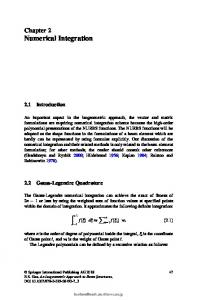
Figure 5.1: Global error as a function of the number of steps for the modified Airy test problem with λ = 1 at time t = 10. The solution computed with 2 11 steps was used as the reference comparison. with (5.3)
A0 (t) =
µ
0 −t2
1 0
¶
and
A1 (t) =
µ
0 −1
1 0
¶
.
The quadratic time dependence is chosen to expose the worst-case cubic error growth as the parameter λ is increased. Figure 5.1 compares the error of different schemes relative to a highly resolved reference computation. The integrals that appear in the Magnus series were evaluated analytically. The fourth order Runge–Kutta is the standard one, where (5.4)
k1 = A(tn ) un ¡ ¢ k2 = A(tn+1/2 ) un + 21 h k1 ¢ ¡ k3 = A(tn+1/2 ) un + 21 h k2 ¢ ¡ k4 = A(tn+1 ) un + h k3 ¡ ¢ un+1 = un + 61 h k1 + 2 (k2 + k3 ) + k4 .
We also included for comparison, the error for the fourth order Lobatto–IIIC
15
Numerical evaluation of the Evans function
0
−2
log10 Error
−4
−6
−8
−10
−12
−14
Runge−Kutta Gauss−Legendre Magnus ref5 0
1
2
3
log
10
λ
4
5
6
7
Figure 5.2: Global error as a function of λ on the interval [0, 10] with 213 time steps. A reference line of slope 5 is shown for comparison. implicit Runge–Kutta method ¡ ¢ k1 = A(tn ) un + h ( 61 k1 − 13 k2 + 16 k3 ) (5.5) ¡ ¢ 5 1 k2 = A(tn+1/2 ) un + h ( 16 k1 + 12 k2 − 12 k3 ) ¢ ¡ k3 = A(tn+1 ) un + h ( 61 k1 + 23 k2 + 61 k3 ¢ ¡ un+1 = un + 61 h k1 + 4 k2 + k3 ,
and the Gauss-Legendre implicit Runge–Kutta method √ ¢ ¡ k1 = A(tn+1/2−√3/6 ) un + h ( 14 k1 + ( 14 − 63 ) k2 ) (5.6) √ ¢ ¡ k2 = A(tn+1/2+√3/6 ) un + h (( 14 + 63 ) k1 + 41 k2 ) ¡ ¢ un+1 = un + 12 h k1 + k2 .
Magnus integrators clearly excel for this type of highly oscillatory problem: their error is at least three orders of magnitude smaller than that of a Runge– Kutta method of the same order. 5.2
Behaviour for large λ
The advantage of the Magnus integrator becomes even more pronounced when λ is increased, i.e. when the system is made more stiff with the time dependence
16
N.D. Aparicio, S.J.A. Malham and M. Oliver
of the vector field left unchanged. For our modified Airy equation (5.1), we have µ ¶ µ ¶ µ ¶ 0 1+λ 0 0 0 0 (5.7) a0 = , a1 = , and a2 = , −(t2 + λ) 0 −2t 0 −1 0 so that the local truncation error for the fourth order Magnus method from (4.13) reads (5.8) h5 (2 [a0 , [a0 , a2 ]] + 3 [a1 , [a1 , a0 ]] + [a0 , [a0 , [a0 , a1 ]]]) + O(h6 ) 720 ¶ µ h5 2t(1 + λ)(t2 + λ) (1 + λ) + O(h6 ) . = 4(1 + λ) −5t2 + λ −2t(1 + λ)(t2 + λ) 720
E2mag =
Hence, E2mag grows cubically with λ while the local truncation error for the fourth order Neumann or explicit Runge–Kutta method is proportional to a 50 , so that E4neu and E4rk grow quintically with λ. These different scalings can be seen in Figure 5.2—though notice that when λ is small all the schemes scale markedly better than expected. This is because on the interval [0, 10] there are many zeros of the solution, the number of which increases with λ. Hence as a function of λ, we might expect the global error to scale better than the local error. Using the convergence criterion (2.14), since kA1 k = 1 and hλ À 1, the Magnus series should no longer be convergent when log λ ≈ 2.9. The ‘spike’ that is observed in Figure 5.2 occurs slightly beyond this value at log λ ≈ 3.3. However this may be accounted for in a slightly smaller value for the commutator constant ν in this system (we examine these points in more detail and the behaviour for larger values of log λ in §5.3). For all the numerical simulations in this section, we evaluated the integrals in the truncated Magnus expansions exactly. This is relatively straightforward for polynomial coefficient problems. However, for more general equations we might need to use numerical quadrature to evaluate the Magnus expansion and this may complicate the form of the local truncation error E2mag . Since our focus later on will be on precomputation schemes we have assumed that the terms in the Magnus expansion will be evaluated to sufficient accuracy so that when the coefficient matrix A1 is constant, the local truncation error E2mag will still be dominated by [a0 , [a0 , [a0 , a2 ]]] and hence λ3 . 5.3
Behaviour for very large λ
As λ becomes very large, a number of interesting effects set in. Although this is not the regime of interest for our application to eigenvalue problems coming from linear stability analysis for reaction-diffusion partial differential equation, we briefly describe the phenomenology, argue that the Magnus integrator remains robust in this regime, and finally point out a better factorization of the flow map that should be applied if this regime is the main focus of interest. A detailed analysis is provided in Appendix A.
17
Numerical evaluation of the Evans function
2
0
−2
−6
log
10
Error
−4
−8
−10
−12
−14
Magnus ref1 ref3 0
2
4
6
8 log10 λ
10
12
14
16
Figure 5.3: Global error as a function of λ for the modified Airy test problem solved with a fourth order Magnus scheme on the interval [0, 1] with 512 time steps. Two reference lines of slopes 1 and 3 are shown for comparison. For λ very large, local truncation error analysis is inappropriate, as Figure 5.3 demonstrates. We can identify several distinct asymptotic regimes. In the first region, where hλ ¿ 1, we see the expected cubic growth in the global error. This is the regime where the crude convergence condition (2.14) is satisfied. The second region, where h2 λ ¿ 1 ¿ hλ, the constant part of the coefficient matrix begins to dominantly determine the form of the solution. In this region, we observe order reduction—the Magnus integrator no longer performs as a fourth order scheme. This is clearly seen in Figure 5.4, which shows our Magnus integrator behaving more like a second order integrator. The third region, where h4 λ ¿ 1 ¿ h2 λ, the scheme behaves as a fourth order Magnus integrator again, the error being linear in λ. Although the higher order terms in the local truncation error would appear to scale very unfavourably with λ, the remarkably good behaviour of the Magnus integrator can be explained by looking primarily at the large λ asymptotics, rather than the small h limit. A careful WKBJ analysis, the details of which are given in Appendix A, reveals that the exact flow-map S(h) over the interval [t, t + h] behaves like (5.9)
S(h) ∼ exp (ha0 ) exp (˜ σ (t, h))
as λ → ∞, where a0 is the constant part in the series expansion of the coefficient
18
N.D. Aparicio, S.J.A. Malham and M. Oliver
log10 Error
log λ = 2
log λ = 3.5
−2
0
−4
−2
−6
−4
−8
−6
−10
−8
−12
−10 Magnus ref4
−14 −16
0
1
Magnus ref2 ref4
−12 2
3
4
5
−14
0
1
log λ = 5
3
4
5
4
5
log λ = 10
2
2
0
0
−2 log10 Error
2
−2
−4 −4 −6 −6
−8
Magnus ref2 ref4
−10 −12
0
1
−8 2 3 log10 Steps
4
5
−10
Magnus ref4 0
1
2 3 log10 Steps
Figure 5.4: Demonstration of order reduction when log λ ≈ 5. The plots show the global error of the fourth order Magnus integrator as a function of the number of steps for the modified Airy test problem on the interval [0, 1] for different fixed values of λ. Two reference lines of slopes −2 and −4 are shown for comparison. matrix A(t + h, λ) defined in (5.7) and σ ˜ (t, h) is given by µ ¶µ ¶ µ ¶ h3 th cos 2µh 0 1 sin 2µh σ ˜ (t, h) = 12 th2 + − −1 0 3 2ν sin 2µh − cos 2µh ¶¶ µ 2¶ µµ µ ¶ h h t sin 2µh 1 − cos 2µh +O + 2 +O . 1 − cos 2µh − sin 2µh 2ν ν ν2 Using this asymptotic form we can show that indeed µ ¶ µ ¶ ¡ 4 ¢ ¡ 2¢ h 1 global (5.10) E =O h λ +O h +O +O λ λ2
for h4 λ ¿ 1 ≈ hλ, where the O(h2 ) term is responsible ¡ ¢ for the behaviour observed in the regime h2 λ ¿ 1 ¿ hλ and the O h4 λ term responsible for that in h4 λ ¿ 1 ¿ h2 λ. For λ À h−4 , all accuracy is lost. However, when
Numerical evaluation of the Evans function
19
hλ ≈ 1 the O(h2 ), O(h/ν) and O(1/ν 2 ) terms are all significant and produce the spiking behaviour observed in that regime. In the large λ regime, the asymptotic form of the solution provided by (5.9) suggests a different numerical scheme, which has been exploited very successfully by Iserles [20] and Degani and Schiff [12]. Decomposing the coefficient matrix A(t + h, λ) into its natural constant and varying parts, (5.11)
A(t + h, λ) = a0 + a ˆ(t, h) ,
we concurrently isolate the part of the coefficient matrix, namely a0 responsible for the frequency oscillations—recall that a0 has pure imaginary eigenvalues scaling linearly with λ. We can then factorize the flow map in the form ˆ S(h) = exp(a0 h)S(h) ,
(5.12)
ˆ where the rescaled fundamental solution S(h) satisfies the differential equation (5.13)
Sˆ0 = exp(−a0 h)ˆ a(t, h) exp(a0 h)Sˆ .
The new coefficient matrix exp(−a0 h)ˆ a(t, h) exp(a0 h) is uniformly bounded in λ, ˆ as are the rescaled solution S(h) and correspondingly the radius of convergence of its Magnus series. 6
The Evans function
6.1
Linear stability of travelling waves
Linear non-autonomous differential equations with parameters arise when constructing the spectrum of a linear elliptic sectorial operator. Such operators are, for example, associated with the problem of linear stability of steady travelling wave solutions to parabolic semilinear systems of partial differential equations (6.1)
Ut = BUξξ + c Uξ + F (U ) ,
where U : R × R+ → Rn has prescribed boundary conditions U (ξ, · ) → U± as ξ → ±∞. B is a constant positive diagonal matrix and F is a smooth bounded function on Rn . The system is written in a frame of reference travelling in the positive x-direction with constant speed c, so that ξ = x − ct. A travelling wave is simply a steady state solution of (6.1) or, in the language of dynamical systems, a homoclinic or heteroclinic orbit of the corresponding steady state ordinary differential equation. Thus, existence of travelling waves can often be shown by topological arguments even when a closed form expression is not available. To analyze the linear stability of a travelling wave Uc (ξ), we look for perturbations of the form (6.2)
ˆ (ξ)eλt , U (ξ, t) = Uc (ξ) + U
20
N.D. Aparicio, S.J.A. Malham and M. Oliver
and linearize (6.1) about Uc . We say that the travelling wave is linearly stable if no part of the spectrum of the linearized right hand side, (6.3)
L = B∂ξξ + c I∂ξ + DF (Uc (ξ))
endowed with homogeneous Dirichlet boundary conditions at ξ = ±∞, is contained in the right complex half–plane. The spectrum of L generally consists of the pure point spectrum—isolated eigenvalues of finite multiplicity—and the essential spectrum. The essential spectrum is contained within the parabolic curves of the continuous spectrum [18]. In many cases the essential spectrum can be shown to be contained in the left-half complex plane and hence does not contribute to linear instability. The task at hand is then to determine the location of the pure point spectrum within a sufficiently large semi-circle in the right-half plane centred at the origin. As the travelling wave is translation invariant, zero is an eigenvalue of L. More generally, we seek values of λ for which there exist non-trivial solutions ˆ : R → Cn to the ordinary differential eigenvalue problem U ˆ (ξ) = λ U ˆ (ξ) , LU
(6.4)
ˆ, U ˆξ ), we can write (6.4) as which vanish as ξ → ±∞. Setting Y = (U Y 0 = A(ξ, λ) Y ,
(6.5)
where A(ξ, λ) ∈ C2n×2n is the matrix of coefficients µ ¶ O I ¡ ¢ A(ξ, λ) = (6.6) . B −1 λ − DF (Uc (ξ)) −c B −1 6.2
The Evans function as a Wronskian
We assume that to the right of the essential spectrum the limiting matrices A± (λ) = limξ→±∞ A(ξ, λ) have k and 2n − k eigenvalues with strictly positive and negative real part, respectively. In other words, there is a k-dimensional subspace of solutions which decay exponentially fast to zero as ξ → −∞, and also a (2n − k)-dimensional subspace of solutions which decay exponentially fast to zero as ξ → +∞. The values of λ for which these subspaces have a non-trivial transverse intersection are the eigenvalues of the linear operator L. The eigenvalue problem (6.5) induces an initial value problem on the exterior Vk 2n power C ,
(6.7a)
Y−0 = A(k) (ξ, λ) Y− ,
lim Y− (ξ) = V− (λ) ,
ξ→−∞
representing the subspace of solutions to (6.5) which decay exponentially to the V2n−k 2n C , left, and a final value problem on (6.7b)
Y+0 = A(2n−k) (ξ, λ)Y+ ,
lim Y+ (ξ) = V+ (λ) ,
ξ→∞
Numerical evaluation of the Evans function
21
representing the subspace of solutions to (6.5) which decay exponentially to the right. The initial value V− (λ) is the eigenvector corresponding the the simple eigenvalue µ− (λ) with the largest positive real part of the limiting induced coefficient matrix A(k) (−∞, λ); the final value V+ (λ) is the eigenvector corresponding to the simple eigenvalue µ+ (λ) with largest negative real part of the limiting induced coefficient matrix A(2n−k) (∞, λ). The two subspaces intersect transversally if and only if the Wronskian determinant Y+ ∧ Y− vanishes. Alexander, Gardner, and Jones [1] define the Evans V2n 2n ∼ function D : C → C = C as the ξ-independent Wronskian
(6.8)
D(λ) = e−
Rξ 0
Tr A(τ,λ)dτ
¡
¢ Y+ (ξ; λ) ∧ Y− (ξ; λ) .
The Evans function is analytic for λ strictly to the right of the essential spectrum. Its zeros correspond to eigenvalues of the linear operator L where the order of each zero determines the algebraic multiplicity of the eigenvalue. In research on Sturm-Liouville problems the Evans function is also known as the miss-distance function. For details see Evans [14], Pryce [36] and Alexander, Gardner and Jones [1]. 6.3
Numerical evaluation
To evaluate the Evans function numerically, we first truncate the infinite ξdomain to a suitably chosen interval [ξ0− , ξ0+ ]. On this interval, we compute, using simple or multiple shooting, the travelling wave to any required accuracy. To avoid integrating exponentially growing solutions in (6.7) which complicate error control when locating the zeros of the Evans function and may lead to floating point overflows, we re-scale ±
Y± (ξ; λ) = W± (ξ; λ) eµ± (λ)(ξ−ξ0 ) .
(6.9)
The rescaled variables W± (ξ; λ) solve (6.7) with modified coefficient matrices A(k) (ξ, λ) − µ− (λ)I and A(2n−k) (ξ, λ) − µ+ (λ)I, respectively. For each value of λ, we numerically solve the equations for W± up to a midpoint ξ∗ ∈ [ξ0− , ξ0+ ] chosen to minimize integration error. It is then usually sufficient to simply evaluate W+ ∧ W− rather than D(λ) as the zeros of the two expressions coincide. To determine the stability of the travelling wave, we can compute D 0 (λ)/D(λ) along the imaginary axis and use the argument principle to determine the number zeros of the Evans function in the right-half plane, and consequently the number of unstable eigenvalues of L. This requires sampling the Evans function for a widespread and sufficiently dense set of points along the imaginary axis. 6.4
Precomputation
Note that the coefficient matrices of the original as well as the induced spectral problem depend linearly on λ. We are therefore in the situation where each step of a one-step method can be written as multiplication with a matrix-valued
22
N.D. Aparicio, S.J.A. Malham and M. Oliver
polynomial in λ or—in case of the Magnus method—the exponential of a matrixvalued polynomial in λ. Precomputing the coefficients can substantially increase efficiency if the Evans function must be evaluated many times with different λ. However, factoring out the exponential growth as in (6.9) substantially reduces the efficiency of precomputation as the dependence of µ± on λ is generally non-polynomial, so that µ± would have to enter as a second parameter. However the favourable stability properties of Magnus methods mean that in practice we can simply divide the solution matrix over each subinterval by the appropriate scalar rescaling factor, as this approximation leaves the location of the zeros invariant. (Choosing to rescale in this way over longer intervals may incur floating point representation problems.) In particular, for a Magnus method we would 1. Precompute the complete set of coefficients (3.13) for each of the intervals [ξ0− , ξ∗ ] and [ξ∗ , ξ0+ ]. 2. Evaluate, for each value of λ, ! ! Ã Ã ± ± ± ± eσN (ξ0 ,ξ1 ;λ) eσN (ξM −1 ,ξM ;λ) ◦ ··· ◦ ◦ V± (λ) . W± (ξ∗ ; λ) ≈ ± ± ± ± eµ± (λ)(ξ1 −ξ0 ) eµ± (λ)(ξM −ξM −1 ) 3. Using these approximations compute W+ ∧ W− . We may also wish to change some other physical parameters in the system. However, since the effort of precomputation increases sharply with the number of parameters and the shape of the travelling wave may depend on these parameters, too, this is best done by recomputing the set of coefficients, or possibly by fixing λ and varying another parameter. 6.5
Pulsating fronts in autocatalysis
As a specific nontrivial example, we study travelling waves in a model of autocatalysis in a medium of infinite extent, (6.10a) (6.10b)
∂t U1 = δ ∂ξξ U1 + c ∂ξ U1 − U1 U2m , ∂t U2 = ∂ξξ U2 + c ∂ξ U2 + U1 U2m .
The fields U1 (ξ, t) and U2 (ξ, t) are the concentrations of the reactant and autocatalyst, respectively. We suppose (U1 , U2 ) approaches the stable homogeneous steady state (0, 1) as ξ → −∞, and the unstable homogeneous steady state (1, 0) as ξ → +∞. The diffusion parameter δ is the ratio of the diffusivity of the reactant to that of the autocatalyst and m is the order of the autocatalytic reaction. This system is globally well-posed for smooth initial data, and any finite δ > 0 and m > 1. Travelling wave solutions satisfy an autonomous nonlinear ordinary differential eigenvalue problem for the wavespeed c. Billingham and Needham [6] proved
Numerical evaluation of the Evans function
23
that, modulo translation, a unique heteroclinic connection between the homogeneous steady states Uc− = (0, 1) as ξ → −∞ and Uc+ = (1, 0) as ξ → +∞ exists for all wave speeds c ∈ [cmin , ∞). Here we are interested in the stability of the exponentially decaying travelling wave of minimum speed cmin . It is the unique heteroclinic connection which lies simultaneously in the one dimensional unstable manifold of Uc− and the two dimensional stable manifold of Uc+ . Figure 6.1 shows the travelling wave computed by a simple shooting algorithm. The linear operator L associated with small perturbations about Uc = (u, v) satisfies all properties previously assumed. The matrix of the corresponding first order eigenvalue problem is 0 0 1 0 0 0 0 1 (6.11) A(ξ, λ) = λ/δ + v m /δ muv m−1 /δ −c/δ 0 . −v m λ − muv m−1 0 −c As in Allen and Bridges [2], we identify induced coefficient matrix in the form
V2
C4 ∼ = C6 and write the resulting (2)
(2)
A(2) (ξ, λ) = A0 (ξ) + λ A1 ,
(6.12) where
0
muv m−1 /δ −muv m−1 (2) A0 (ξ) = −v m /δ vm 0
and
(2)
A1
0 −c/δ 0 0 0 vm
1 0 −c 0 0 v m /δ
0 0 1 = −1/δ 0 0
−1 0 0 −c/δ 0 muv m−1
0 0 0 0 0 0 0 0 0 0 0 1/δ
0 0 0 0 0 −1
0 0 0 0 −c muv m−1 /δ
0 0 1 −1 0 −c(1 + δ)/δ
0 0 0 0 0 0 0 0 0 0 0 0
A so-called pulsating instability occurs when δ < 1 is sufficiently small and m is sufficiently large. For δ fixed and m increasing, a complex conjugate pair of eigenvalues crosses into the right-half λ-plane signifying the onset of instability via a Hopf bifurcation [4]. Figure 6.2 clearly shows the onset of this instability as m is increased from 8 to 9 and δ = 0.1. 6.6
Comparing Magnus and Runge–Kutta integrators
When detecting and locating the unstable eigenvalues, we particularly need to sample the Evans function along the imaginary λ-axis as explained in Section 6.3 (the symmetry properties of the Evans function about the real λ-axis mean that
24
N.D. Aparicio, S.J.A. Malham and M. Oliver
1.2
1
0.8 u(ξ) v(ξ) w(ξ)
Uc (ξ)
0.6
0.4
0.2
0
−0.2 −15
−10
−5
0 ξ
5
10
15
Figure 6.1: The travelling wave solution Uc (ξ) = (u, v) for δ = 0.1 and m = 9. The bottom curve is w = v 0 . -0.04
m=8 0
0.1
0.04
-0.04
m=9 0
0.04
0.1 0.1
0
0
0.1
0
0
-0.1 -0.1
-0.1
-0.1
-0.04
0
0.04
-0.04
0
0.04
Figure 6.2: Zero contours lines of the real and imaginary parts of the Evans function for problem (6.10) with δ = 0.1 and m = 8 (left) and m = 9 (right). Solid lines correspond to zero contours of Re D(λ), dashed lines to Im D(λ). Hence, the Evans function is zero where the lines intersect. We see that a complex-conjugate pair of eigenvalues crosses into the right-half plane as m increases, indicating the onset of instability. Note that due to translational invariance, the origin is always an eigenvalue. Also note that there is a branch cut along part of the negative real axis and the zero contour of Im D(λ) there should be ignored (a sign-changing jump occurs).
Numerical evaluation of the Evans function
25
evaluation is only required along the positive imaginary axis). In the case that zeros in the right half plane are detected, we may want to localize the region of integration and finally use root finding methods to determine the exact location. Note that if A(2) (ξ + h, λ) has an expansion of the form (6.13)
A(2) (ξ + h, λ) = a ˆ0 + a ˆ1 h + a ˆ 2 h2 + . . . , (2)
(2)
then the structure of A0 (ξ) and nilpotency of A1 (2) [ˆ a1 , A1 ] (2) [ˆ a2 , A1 ] (2) (2) (2) [A1 , [A1 , [A0 (ξ), a ˆ1 ]]]
of degree 2, imply that
= 0, = 0, ≡ 0.
So that in particular, the terms [ˆ a0 , [ˆ a0 , a ˆ2 ]] and [ˆ a0 , [ˆ a0 , [ˆ a0 , a ˆ1 ]]] in the local truncation error (4.13) only grow linearly with |λ|, while the term [ˆ a1 , [ˆ a1 , a ˆ0 ]] is independent of |λ|. Hence for h|λ| ¿ 1 the local truncation error only grows linearly rather than cubically with |λ|—in fact the global error in Figure 6.4 scales slightly better than linearly with |λ|. There are two regimes that can present difficulties for the numerical scheme. First, when λ is large along the positive imaginary axis, the system has eigenvalues with large negative real part, so that integrators that are not A-stable will eventually lose stability. Second, in the presence of higher bound states or in the vicinity of the essential spectrum, the system develops eigenvalues with a large imaginary, or even positive component. This regime taxes both accuracy and stability of the integrator. We will now see how the Magnus integrator performs in each of these two regimes. 6.7
Comparison for large |λ|
When λ is purely imaginary but large in magnitude, RK4 becomes unstable— its domain of stability is shown in Figure 6.3. In fact, the magnitude of the √ dominant eigenvalue of maximum magnitude of the system grows like y for large λ = iy, and either explicit Magnus or an implicit numerical integrator of finite difference type must be used. We thus compare the performance of the Magnus integrator with Lobatto–IIIC and Gauss-Legendre of the same order. Figure 6.4 shows that the Magnus integrator is doing quite well, although its errors are an order of magnitude above the other two. This case is the “boring” regime—the solution is large in magnitude, but almost constant; traditional integrators do well in this case, and are clearly cheaper, too. (We also remark that Allen and Bridges [2] have shown that Gauss-Legendre can be made even more efficient by taking advantage of the block matrix structure of this system.) For even larger values of |λ| there is an efficient order 1/|λ| asymptotic approximation (see (B.4) in Appendix B) which will give an error of order 10−n when |λ| is larger than 10n . For larger values of |λ|—where the graph is roughly flat, higher order terms in the expansion become important and reduction of order is occurring. When |λ| is larger still, the global error in Figure 6.4 grows like |λ|3/2 .
26
N.D. Aparicio, S.J.A. Malham and M. Oliver
-7
0
7
-30
7
7
0
0
-7
-7 -7
0
7
0
30
30
30
0
0
-30
-30 -30
0
30
Figure 6.3: The closed regions of the complex λ-plane where all the eigenvalues of the coefficient matrices A(2) (+∞, λ) − µ+ (λ)I (scaled by the steplength factor −h) lie in the region of absolute stability of RK4 (on the left δ = 0.1 and h = 17/128, on the right δ = 0.005 and h = 17/1024). The longer boundary to the bottom, right and top in these plots indicates where one of the eigenvalues becomes too large in magnitude. The indented boundary on the left indicates where the real part of one of the eigenvalues becomes positive (and where the Gauss-Legendre method becomes unstable—it lies just to the left of the right–hand boundary of the essential spectrum). 6.8
Comparison near the essential spectrum
In the second important regime Magnus integrators not only do well, but outperform Lobatto–IIIC and Gauss–Legendre by a clear margin. Since our eigenvalue problem has no apparent higher bound states, we compare all three integrators as λ traverses into the indented boundary in the right-hand plot in Figure 6.3. Figure 6.5 shows that the Magnus integrator not only scales extremely robustly throughout, but outperforms the two implicit schemes as we move inside the essential spectrum. The robustness of the Magnus methods should make it widely applicable to spectral problems. For example, the eigenvalues of the coefficient matrix may change magnitude and their real parts may change sign as ξ varies in the interval of integration. Explicit and also implicit Runge-Kutta methods will not work reliably without adaptive stepsize control, whereas Magnus integrators remain unaffected by such variations. We expect that this is important when determining stability of multi-bump pulses, multi-phase travelling fronts or when computing higher bound states of coupled Schr¨odinger operators. 7
Conclusions and outlook
We have compared standard Runge–Kutta schemes with a Magnus integrator of the same order for the task of numerical evaluation of the Evans function. We found that, on the one hand, precomputation alone does not position the Magnus
27
Numerical evaluation of the Evans function
0 Magnus Gauss−Legendre Lobatto−IIIC
−1
−2
log10 Error
−3
−4
−5
−6
−7
−8
−9
0
1
2
3
4
5 log
10
6
7
8
9
y
Figure 6.4: Numerical error when computing the Evans function D(iy) for δ = 0.1 and m = 8.3 along the imaginary axis using fourth order Magnus, Lobatto–IIIC and Gauss-Legendre methods. The top set were computed with 128 steps, so h = 17/128 for [ξ∗ , ξ0+ ] = [−7, 10], whilst the bottom set correspond to 512 steps, h = 17/512. A typical Nyquist plot would have y range from 10 −4 to 106 . In the lower set of plots, for log λ > 6 the coefficient matrix of the linear system of equations to be solved at each step for the Gauss-Legendre and Lobatto–IIIC becomes ill–conditioned. integrator ahead of Runge–Kutta methods. Although the Magnus integrator may be more accurate for a given step size, the cost of exponentiation will dominate the computational expense in many situations. On the other hand, Magnus integrators are extremely robust. Their performance remains uniformly good across regimes where the equations become stiff and, correspondingly, Runge–Kutta methods fare arbitrarily poorly. The distinct advantages of Magnus integrators are 1. Unconditional stability, 2. Superior performance in highly oscillatory regimes, 3. Possibility of a priori stepsize control. Items 2 and 3 reflect that error bounds for Magnus methods depend only on low order derivatives of the matrix A, not—as for Runge–Kutta schemes—on derivatives of the solution (e.g., for a Runge–Kutta method of order N the
28
N.D. Aparicio, S.J.A. Malham and M. Oliver
λ=−1+i
λ=−1.15+i
log10 Error
0
0 −5 −5
−10
log10 Error
5
1
1.5
2 λ=−1.05+i
2.5
3
−10
0
5
−5
0
−10
1
1.5
2 λ=−1.1+i
2.5
3
0
−5
1
1.5
2 λ=−1.2+i
2.5
3
1
1.5
2 λ=−1.25+i
2.5
3
1
1.5
2 Steps
2.5
3
5
log10 Error
−2 −4
0
−6 −8
1
1.5 log
10
2 Steps
2.5
3
−5
log
10
Figure 6.5: Global error as a function of the number of steps computed for different values of λ = x + i over the interval [ξ∗ , ξ0+ ] = [−7, 10] with δ = 0.005 and m = 12. We compare the fourth order Magnus (¦), Lobatto–IIIC (∗) and Gauss–Legendre (¤). As x decreases, the real part of one of the eigenvalues of A(2) (+∞, λ) − µ+ (λ)I becomes positive and as we move further to the left we begin see the Magnus integrator outperform both of the implicit schemes. error effectively depends on N + 1 derivatives of A). Therefore, performance and, correspondingly, the choice of optimal step size remain uniform over any bounded region of parameter space. Moreover, while stepsize control for Runge– Kutta is crucial to ensure stability, performance of Magnus methods is relatively insensitive to the choice of step sizes—in the problems we studied performance with optimal step size control remains within a factor 2 from performance with equidistant partition. Since much of the performance balance hinges on the efficiency of matrix exponentiation which we did not attempt to explicitly optimize, we cannot yet state a quantitative cross-over point for Runge–Kutta vs. Magnus. However, we believe that Magnus integrators could become method of choice for this type of problem due to their robust and predictable behaviour.
29
Numerical evaluation of the Evans function
Further progress may be made in the following directions: Evaluation of the semi-infinite exponential tails by analytically computable Magnus steps, the combination of the Magnus series with an operator splitting approach, so that some of the matrix exponentials can also be precomputed, and the use of expansions with respect to model parameters as a tool for proving properties of the Evans function. Finally, the use of Neumann series integrators has very recently proved successful for certain large, highly oscillatory systems—see Iserles [21]— and implications for systems with parameters remain to be explored. A
Appendix: WKBJ analysis for the modified Airy equation
A.1
WKBJ solution
Setting ν = 1 + λ, we decompose the coefficient matrix for the modified Airy equation (5.1) as (A.1)
A(t + h, ν) = a0 (t, ν) + a ˆ(t, h) ,
where (A.2)
a0 (t, ν) =
µ
0 1 − ν − t2
ν 0
¶
and a ˆ(t, h) =
µ
0 −2th − h2
0 0
¶
.
The eigenvalues of a0 are (A.3)
µ± = ±iν
r
1+
t2 − 1 ≡ ±iµ , ν
and the change of coordinates that diagonalizes a0 has the asymptotic form (A.4a)
µ 1 1 X=√ 2 i (A.4b) µ 1 1 X −1 = √ 2 1
¶ µ t2 − 1 −1 1 + √ −i i 4 2ν
¶ µ (t2 − 1)2 −1 3 √ + −i 32 2ν 2 −5i
µ ¶ t2 − 1 −1 −i − √ i 4 2ν −1
µ ¶ (t2 − 1)2 1 −i √ − i 32 2ν 2 1
¶ µ ¶ 1 3 +O , 5i ν3
¶ µ ¶ 1 7i , +O −7i ν3
when ν is large; we write D = X −1 a0 X = diag{iµ, −iµ}. Following Iserles [20] and J´odar and Marletta [26], we factorize the flow map in the form (A.5)
˜ S(h) = X exp(Dh) S(h) ,
The rescaled flow-map S˜ must satisfy the initial value problem (A.6)
˜ h) S˜ , S˜0 = A(t,
˜ S(0) = X −1 ,
where ˜ h) = exp(−Dh) X −1 a (A.7) A(t, ˆ(t, h) X exp(Dh) µ ¶ µµ t2 − 1 1 2 1 = 2 i(2th + h ) 1 − −e2iµh 2ν
e−2iµh −1
¶
+O
µ
h ν2
¶¶
.
30
N.D. Aparicio, S.J.A. Malham and M. Oliver
˜ we find, using the Riemann– Computing the first term of the Magnus series for S, Lebesgue Lemma, that Z
h
˜ h1 ) dh1 A(t, µ ¶µ µ ¶ ¶ h3 th 1 0 0 e−2iµh 2 1 = 2 i th + − 0 −1 0 3 2ν e2iµh ¶ µ ¶ µ ¶ µ h h2 it 0 e−2iµh − 1 +O . +O + 2 2iµh −(e − 1) 0 4ν ν ν2 ¡ ¢ All higher order terms in the Magnus series are are O h2 ν −1 . Reverting to the original flow map, we find µ µ 2 ¶¶ h (A.9) X −1 S(h) = X exp(Dh) exp s˜1 + O ν µ µ 2 ¶¶ h = X exp(Dh) X −1 X exp s˜1 + O X −1 ν µ µ 2 ¶¶ h = exp(a0 h) exp X s˜1 X −1 + O ν (A.8)
s˜1 =
0
= exp(a0 h) exp(˜ σ (t, h)) ,
where ¶ ¶ ¶µ µ th cos 2µh h3 0 1 sin 2µh σ ˜ (t, h) = − th + −1 0 3 2ν sin 2µh − cos 2µh µµ µ ¶ ¶¶ µ 2¶ t h h sin 2µh 1 − cos 2µh + 2 +O . +O 1 − cos 2µh − sin 2µh 2ν ν ν2 1 2
µ
2
This yields the asymptotic formula (5.9) quoted in the main text. A.2
Fourth order Magnus asymptotic form
The fourth order Magnus integrator takes the explicit form (A.10)
S4mag = exp(s1 + s2 ) ,
where (A.11)
s 1 + s2 = h
µ
H1 ≡ th +
h2 3
ν H2 1 − ν − t 2 − H1
ν −ν H2
¶
with (A.12)
and
H2 ≡
th2 h3 + . 6 12
31
Numerical evaluation of the Evans function
The eigenvalues of the matrix s1 + s2 are (A.13)
(A.14)
µmag ±
¶1 µ ¶1 2 t2 − 1 2 ν H22 H1 = ±iνh 1 + − 2 1+ 2 ν t −1+ν t −1+ν µ ¶ µ 4¶ µ ¶ h h 2 8 1 1 H1 − 2 H2 + O + O 2 + O(h ) = hµ± 1 + 2 ν ν ν µ 2¶ ¢ ¡ h + O(h5 ) , = ±ih µ + 21 H1 − 12 ν H22 + O ν µ
≡ ±iµmag ,
where we suppose that h ¿ 1, ν À 1 with 1/ν = O(h) and, in the last step, we have used that µ± = ±iν + O(1). Writing D mag = diag{iµmag , −iµmag } and comparing with (A.8), we obtain ¶ µ ¶ µ th 1 0 0 e−2iµh + (A.15) Dmag = Dh + s˜1 − 21 iνhH22 0 −1 0 2ν e2iµh ¶ µ −2iµh it 0 e −1 − 2 −(e2iµh − 1) 0 4ν µ 2¶ µ ¶ h h +O +O + O(h5 ) . ν ν2 The change of variables that diagonalizes s1 + s2 can be written in the nonnormalized asymptotic form ¶ ¶ µ µ 1 H1 −1 −1 H2 0 0 (A.16a) +√ X mag =X − √ i −i 2 1 1 2 4ν µ 2¶ µ ¶ µ ¶ ¡ 4¢ h h 1 +O h +O +O + O , 2 ν ν ν3 µ ¶ µ ¶ H2 −1 0 1 H1 1 i −1 (A.16b) (X mag ) =X −1 + i √ +√ 2 1 0 2 4ν 1 −i µ 2¶ µ ¶ µ ¶ ¡ 4¢ h h 1 +O h +O +O + O . ν ν2 ν3 Hence,
(A.17)
S4mag (h) = exp(s1 + s2 ) = X mag exp (D mag ) (X mag )
−1
¶ 1 0 = X exp (D ) X + H2 sin(µ ) 0 −1 µ ¶ µ 2¶ ¡ 4¢ h H1 0 1 mag sin(µ ) +O h +O − 1 0 ν ν µ ¶ µ ¶ h 1 +O +O . ν2 ν3 mag
−1
mag
µ
32
N.D. Aparicio, S.J.A. Malham and M. Oliver
A.3
Local asymptotic error estimate for the fourth order Magnus scheme
We compare exact solution in its WKBJ asymptotic form—the first line of equation (A.9)—with the asymptotic expression for the fourth order Magnus scheme, (A.18)
µ µ 2 ¶¶ h S(h) − S4mag (h) = X exp(Dh) exp s˜1 + O X −1 − S4mag (h) ν ¸ · µ µ 2 ¶¶ h − exp (D mag ) X −1 = X exp(Dh) exp s˜1 + O ν ¶ µ ¶ µ H1 0 1 1 0 sin(µmag ) + − H2 sin(µmag ) 1 0 0 −1 ν µ 2¶ µ ¶ µ ¶ ¡ 4¢ h 1 h +O h +O +O . +O ν ν2 ν3
The first term on the right can be written as · µ µ 2 ¶¶ ¸ h (A.19) X exp (D mag ) exp (Dh − D mag ) exp s˜1 + O − I X −1 , ν so that, by expanding the two exponentials inside the square bracket, and using the expression for D mag from (A.15), (A.20)
E loc ≡ S(h) − S4mag (h) =
E1loc +O
where E1loc E2loc E3loc E4loc
+ µ
E2loc 1 ν3
¶
+
E3loc
+
E4loc
5
+ O(h ) + O
µ
h2 ν
¶
+O
µ
h ν2
¶
¡ ¢ ¡ ¢ + O νh7 + O ν 2 h10 ,
µ
¶ sin µmag − cos µmag ≡ cos µmag sin µmag µ ¶ 1 0 mag ≡ −H2 sin(µ ) 0 −1 µ µ ¶ ¶ th cos(2µh − µmag ) H1 sin(2µh − µmag ) 0 1 mag sin(µ ) − ≡ 1 0 ν 2ν sin(2µh − µmag ) − cos(2µh − µmag ) ¶ µ it sin(µmag − 2µh) − sin µmag cos(µmag − 2µh) − cos µmag . ≡ 2 cos(µmag − 2µh) − cos µmag − sin(µmag − 2µh) + sin µmag 4ν − 21 νhH22
Hence, E1loc = O(νh5 ) is the dominant error term in the regime h5 ν ¿ 1 ¿ h3 ν; E2loc = O(h2 ) is the dominant error term in the regime h3 ν ¿ 1 ¿ hν. Figure A.1 shows that these leading order error terms are good error indicators even across the transitions between the different asymptotic regimes. The last two error terms, E3loc = O(h/ν) and E4loc = O(1/ν 2 ) become significant in comparison with E2loc when hν ≈ 1 and contribute to the global error in this regime.
33
Numerical evaluation of the Evans function
2
0
−2
log10 Error
−4
−6
−8
−10
−12 local truncation error local error component ||E2|| local error component ||E1||
−14
numerical experiment −16
0
2
4
6
8
log10 ν
10
12
14
16
18
Figure A.1: Local error indicators for the toy modified Airy equation in three different asymptotic regimes. When hν ¿ 1, the error is dominated by the local truncation error. When h3 ν ¿ 1 ¿ hν, the error is dominated by E2loc ; for h5 ν ¿ 1 ¿ h3 ν it is dominated by E1loc . The bottom graph shows the actual computed error for comparison. The graphs for E1loc and E2loc are shifted up by 3 units for better legibility; the actual curves lie on top of each other for large stretches. Parameters are t = 0.5 and h = 1/512. A.4
Global error
In the regime h3 ν ¿ 1 ¿ hν, for example where order reduction is observed, the local error is dominated by µ ¶ 1 0 (A.21) E2loc = −H2 sin(µmag ) = O(h2 ) , 0 −1 while the global error is also of order h2 ; see Figure 5.4. Since E2 is varying slowly relative to the oscillatory solution, local error contributions partially cancel out over many solution periods. This is made explicit in the following. Let Y (t) ≡ S(s, t) Y (s), h = T /N , and tn = nh, so that (A.22)
S(0, T ) =
0 Y
n=N −1
S(tn , tn+1 ) ,
34
N.D. Aparicio, S.J.A. Malham and M. Oliver
with a corresponding expression for S mag . Hence, E global = S(0, T ) − S mag (0, T ) =
n=0 Y
N −1
(A.23)
=
N −1 X n=0
¡
¢ S mag (tn , tn+1 ) + E loc (tn , tn+1 ) − S mag (0, T )
¡ ¢ S mag (tn+1 , T ) E(tn , tn+1 ) S mag (0, tn ) + O kE loc k2 /h .
In the following we derive the explicit leading order asymptotics for the global error. First, recall that (A.24)
S mag = X mag exp(D mag ) (X mag )
−1
.
Moreover, X mag and (X mag )−1 as defined by (A.16) are functions of t, which satisfy µ 2¶ µ ¶ ¡ mag ¢−1 mag ¡ ¢ h h (A.25) X (tn+1 ) X (tn ) = I + O h3 + O +O . ν ν2 We use this observation to conclude that S mag (0, T ) =
0 Y
S mag (tn , tn+1 )
n=N −1
=
0 Y
n=N −1
(A.26) where (A.27)
¡ ¢ −1 X mag (tn ) exp Dmag (tn ) (X mag (tn ))
¡ ¢ −1 = X mag (tN −1 ) exp Dmag (0, T ) (X mag (0)) µ ¶ µ ¶ h 1 + O(h2 ) + O +O ν ν2 µ ¶ ¡ ¢ 1 , = X0 exp Dmag (0, T ) X0−1 + O(h2 ) + O ν
D mag (0, T ) ≡
N −1 X
D(tn ) ,
n=0
and we replaced, consistent to the order shown, X mag (tN −1 ) and (X mag (0)) by µ µ ¶ ¶ 1 1 1 1 1 −i −1 √ √ and X0 = . (A.28) X0 = 2 i −i 2 1 i
−1
35
Numerical evaluation of the Evans function
We now plug (A.26) back into (A.23), (A.29)
E
global
= X0
·NX −1 n=0
¡
· exp D
mag
¡ ¢ exp Dmag (tn+1 , T ) X0−1 E loc (tn , tn+1 ) X0
(0, tn )
¢
¸
¡ ¢ ¡ ¢ X0−1 + O kE loc k2 /h + O νh3 + O
µ
h2 ν
¶
.
This formula is now used to compute, for each of the components of the local error, its corresponding contribution to the global error. For E1loc we see that ÃN −1 µ ¶! X exp(iα ) 0 global n H22 (tn ) X0−1 , (A.30) E1 = 12 iνhX0 0 − exp(−iαn ) n=0
where (recall tj = jh) αn =
N −1 X
µmag (tj )
j=0
=
N −1 µ X j=0
νh −
2 1 2 h(tj
− 1) +
2 1 2 tj h
µ ¶¶ h + O(h ) + O ν 3
(N − 1)N (2N − 1) 1 3 (N − 1)N + 2h + O(h2 ) + O 6 2 µ ¶ 1 . = (ν + 21 )T − 61 T 3 + O(h2 ) + O ν
= νh(N − 1) − 12 h3
µ ¶ 1 ν
Inserting this into (A.30), we find (A.31)
E1global = −
µ 1 sin αn νh4 T 3 cos αn 216
− cos αn sin αn
¶
+ O(h5 ) .
Similarly, plugging in the expression for E2loc into (A.29), we obtain µ ¶ N −1 X ¡ ¢ − cos σn sin σn (A.32) E2global = H2 (tn ) sin µmag (tn ) , sin σn cos σn n=0
where
(A.33)
σn =
N −1 X
j=n+1
(A.34)
= (ν +
µmag (tj ) −
1 2 )(T
n−1 X
µmag (tj )
j=0
− 2tn ) −
1 3 6T
+
1 3 3 tn
+
1 2 2 tn h
µ ¶ 1 + O(h ) + O . ν 2
To compute the asymptotic behaviour of E2global , note that ¡ ¢ ¡ ¢ sin µmag (t) = sin νh + 21 h(t2 − 1) + O(h2 ) ¢ ¡ ¢ ¡ ¢ ¡ (A.35) = sin νh + cos νh sin 12 h(t2 − 1) + O(h) ,
36
N.D. Aparicio, S.J.A. Malham and M. Oliver
and therefore h
N −1 X n=0
¢ ¡ ¢ ¡ tn sin µmag (tn ) exp ±iσn
¡ ¢ = sin νh ¡
Z
+ cos νh
T
0
¢
Z
¡ ¢ τ exp (ν + 12 )(T − 2τ ) − 16 T 3 + 13 τ 3 + 21 τ 2 h + O(h2 ) dτ T
τ sin
¡1
2 h(τ
2
¢ − 1) ·
¡0 ¢ · exp (ν + 12 )(T − 2τ ) − 61 T 3 + 13 τ 3 + 21 τ 2 h + O(h2 ) dτ + O(h) ,
where, consistent with the order of the approximation, we have replaced the sum in (A.32) with an integral, and each integral is of the form (A.36)
e
1 1 ±i(ν+ 2 )T − 6 T 3
Z
T
g(t) e∓2iντ dt , 0
with g(t) a continuous function. By the Riemann–Lebesgue lemma, this expression is of order 1/ν. This proves that µ ¶ ¡ ¢ h (A.37) E2global = O h2 + O . ν
Similar arguments yield the global error contributions corresponding to the local error components E3loc and E4loc µ N −1 ¡ ¢ sin σn 1 X H1 (tn ) sin µmag (tn ) cos σn ν n=0 ¶ µ N −1 h X − cos βn sin βn + tn sin βn cos βn 2ν n=0 µ ¶ µ ¶ 1 h =O +O , ν2 ν
E3global =
cos σn − sin σn
¶
where βn ≡ σn − 2µh + µmag (tn ) and E4global
µ N −1 1 X sin βn − sin γn tn =− 2 cos βn − cos γn 4ν n=0 µ ¶ µ ¶ 1 1 =O + O , hν 2 ν2
cos βn − cos γn − sin βn + sin γn
¶
where γn = σn + µmag (tn ). In Figure A.2 we compare the global error components above against the numerically computed error.
37
Numerical evaluation of the Evans function
2
0
−4
−6
log
10
Global error
−2
−8
−10 numerical experiment ||E1|| ||E +E || 2 3 ||E4||
−12
−14
0
2
4
6
8 log10 ν
10
12
14
16
Figure A.2: Global error indicators for the toy modified Airy equation in three different asymptotic regimes. When h4 ν ¿ 1 ¿ h2 ν, the error is dominated by E1global ; for h2 ν ¿ 1 ¿ hν it is dominated by E2global . When hν = ord(1) then the global error terms E3global and E4global are similar in magnitude to E2global . The bottom graph shows the actual computed error for comparison. The graphs for Eiglobal , i = 1, . . . , 4 are shifted up by 3 units for better legibility; the actual curves lie on top of each other for large stretches. Parameters are t = 1 and h = 1/512. B
Appendix: Asymptotic approximations for Evans function
We can derive asymptotic approximations valid p for large |λ| for solutions to |λ| ξ, we find that the new the eigenvalue problem (6.4). Rescaling z = fundamental matrix S(z, λ) satisfies the system ˜ λ) S , S 0 = A(z,
(B.1) where (B.2)
˜ λ) = A(z,
µ
B
¡ −1
O¡ p ¢ ¢ Iei argλ − DF Uc (z/ |λ|) /|λ|
I p −c B −1 / |λ|
˜ λ) approaches the constant coefficient matrix In the limit |λ| → ∞, A(z, µ ¶ O I (B.3) A∞ = i argλ −1 . e B O
¶
.
38
N.D. Aparicio, S.J.A. Malham and M. Oliver
In particular, when λ → i∞, we can show that the Evans function is given √ by ˜ the determinant of the eigenvectors of A∞ . More explicitly, D(iy) → −4i δ as y → +∞; see, for example, Sandstede [38]. Further, S(z, λ) has an asymptotic expansion of the form ¶ µ S1 (z) S2 (z) 1 (B.4) S(z, λ) = exp(zA∞ ) + + , + O 1 3 |λ| |λ| 2 |λ| 2 where (B.5)
S1 (z) = z exp(zA∞ ) · dexp−zA∞ (A˜1 ) ,
and S2 (z) satisfies the differential equation (B.6)
S20 = A∞ S2 + A˜1 S1 + A˜2 (z) exp(zA∞ ) ,
1 and where A˜1 and A˜2 (z) are the coefficients of 1/|λ| 2 and 1/|λ| in the expansion ˜ λ): of A(z, µ ¶ µ ¶ O p O O O ˜ ˜ ¢ (B.7) A1 = and A2 (z) = . O −cB −1 −DF (Uc (z/ |λ|)) O
We can solve (B.6) through the variation of constants formula, but evaluation of S2 (z) will require knowledge of A˜2 (z) and hence numerical evaluation of the travelling wave Uc . This means that effective analytical estimates for S(z, λ) incur an order 1/|λ| error. Acknowledgment We thank Tom Bridges, Arieh Iserles, Frank Janssens, Gabriel Lord, Christian Lubich, Jitse Niesen, Brynjulf Owren and Antonella Zanna for many stimulating discussions. We would also like to thank the anonymous referees for their numerous suggestions for improvement of the original manuscript. This work was supported by an EPSRC First Grant no. GR/S22134/01, the Nuffield Foundation grant no. SCI/180/97/129/G, the London Mathematical Society via a Scheme 2 visitors grant no. 611, the MASIE European Training and Mobility Network, and German Science Foundation SFB 382. REFERENCES 1. J. C. Alexander, R. Gardner and C. K. R. T. Jones, A topological invariant arising in the stability analysis of traveling waves, J. Reine Angew. Math., 410 (1990), pp. 167–212. 2. L. Allen and T. J. Bridges, Numerical exterior algebra and the compound matrix method, Numer. Math., 92 (2002), pp. 197-232. 3. H. F. Baker, On the integration of linear differential equations, Proc. London Math. Soc., 35 (1903), pp. 333–378. 4. N. J. Balmforth, R. V. Craster and S. J. A. Malham, Unsteady fronts in an autocatalytic system, Proc. R. Soc. Lond. A, 455 (1999), pp. 1401–1433.
Numerical evaluation of the Evans function
39
5. I. Bialynicki-Birula, B. Mielnik and J. Plebanski, Explicit solution of the continuous Baker-Campbell-Hausdorff problem and a new expression for the phase operator, Annals of Physics, 51 (1969), pp. 187–200. 6. J. Billingham and D. Needham, The development of travelling waves in quadratic and cubic autocatalysis with unequal diffusion rates, I and II, Phil. Trans. R. Soc. Lond. A, 334 (1991), pp. 1–124, and 336 (1991), pp. 497–539. 7. S. Blanes, F. Casas and J. Ros, Optimized geometric integrators of high order for linear differential equations, BIT, 42 (2002), pp. 262–284. 8. S. Blanes, F. Casas, J. A. Oteo and J. Ros, Magnus and Fer expansions for matrix differential equations: the convergence problems, J. Phys A: Math. Gen., 31 (1998), pp. 259–268. 9. B. Chanane, Fleiss series approach to the computation of the eigenvalues of fourth– order Sturm–Liouville problems, Appl. Math. Lett. , 15 (2002), pp. 459–463. 10. K. T. Chen, Integration of paths, geometric invariants and a generalized Baker– Hausdorff formula, Annals of Mathematics, 65(1) (1957), pp. 163–178. 11. S. Coombes and M. R. Owen, Evans function for integral neural field equations with heaviside firing rate function, submitted to SIAM J. Appl. Dyn. Syst. (2004). 12. I. Degani and J. Schiff, RCMS: right correction Magnus series approach for integration of linear ordinary differential equations with highly oscillatory solution, preprint. 13. F. J. Dyson, The radiation theories of Tomonaga, Schwinger, and Feynman, Physical Review, 75(3) (1949), pp. 486–502. 14. J. W. Evans, Nerve axon equations, IV: The stable and unstable impulse. Indiana Univ. Math. J., 24 (1975), pp. 1169–1190. 15. L. Greenberg and M. Marletta, Numerical solution of non-self-adjoint SturmLiouville problems and related systems, SIAM J. Numer. Anal. , 38(6) (2001), pp. 1800–1845. 16. E. Hairer, S. P. Nørsett and G. Wanner, Solving ordinary differential equations I, Springer-Verlag, Springer Series in Computational Mathematics 8, 1987. 17. E. Hairer and G. Wanner, Solving ordinary differential equations II, SpringerVerlag, Springer Series in Computational Mathematics 14, 1991. 18. D. Henry, Geometric theory of semilinear parabolic equations, Springer-Verlag, Lecture Notes in Mathematics 840, 1981. 19. M. Hochbruck and C. Lubich, On Magnus integrators for time-dependent Schr¨ odinger equations, SIAM J. Numer. Anal., 41 (2003), pp. 945–963. 20. A. Iserles, Think globally, act locally: solving highly-oscillatory ordinary differential equations, Appl. Numer. Math., 43 (2002), pp. 145–160. 21. A. Iserles, On the method of Neumann series for highly oscillatory equations, submitted to BIT (2004). 22. A. Iserles, A. Marthinsen and S. P. Nørsett, On the implementation of the method of Magnus series for linear differential equations, BIT, 39 (1999), pp. 281–304. 23. A. Iserles, H. Z. Munthe-Kaas, S. P. Nørsett and A. Zanna, Lie-group methods, Acta Numerica, (2000), pp. 215–365. 24. A. Iserles and S. P. Nørsett, On the solution of linear differential equations in Lie groups, Phil. Trans. R. Soc. Lond. A, 357 (1999), pp. 983–1019. 25. A. Iserles and A. Zanna, Efficient computation of the matrix exponential by generalized polar decompositions, Technical report 2002/NA09, DAMTP, University of Cambridge, 2002.
40
N.D. Aparicio, S.J.A. Malham and M. Oliver
26. L. J´ odar and M. Marletta, Solving ODEs arising from non-selfadjoint Hamiltonian eigenproblems, Adv. Comput. Math. , 13 (2000), pp. 231–256. 27. T. Kapitula, The Evans function and generalized Melnikov integrals, SIAM J. Math. Anal., 30 (1998), pp. 273–297. 28. D. E. Knuth, The art of computer programming, Second Edition, Addison-Wesley Publishing Company, 1981. 29. W. Magnus, On the exponential solution of differential equations for a linear operator, Comm. Pure Appl. Math., 7 (1954), pp. 649–673. 30. P.-C. Moan, Efficient approximation of Sturm-Liouville problems using Lie-group methods, Technical report 1998/NA11, DAMTP, University of Cambridge, 1998. 31. P.-C. Moan, On backward error analysis and Nekhoroshev stability in the numerical analysis of conservative systems of ODEs, PhD Thesis, University of Cambridge, 2002. 32. C. Moler and C. Van Loan, Nineteen dubious ways to compute the exponential of a matrix, twenty-five years later, SIAM Review, 45 (2003), pp. 3–49. 33. H. Munthe-Kaas and B. Owren, Computations in a free Lie algebra, Phil. Trans. R. Soc. Lond. A, 357 (1999), pp. 957–981. 34. G. Peano, Int´egration par s´eries des ´equations diff´erentielles lin´eaires, Mathematische Annalen, XXXII (1888), pp. 450–457. 35. R. L. Pego and M. I. Weinstein, Eigenvalues, and instabilities of solitary waves, Phil. Trans. R. Soc. Lond. A, 340 (1992), pp. 47–94. 36. J. D. Pryce, Numerical solution of Sturm–Liouville problems, Monographs on Numerical Analysis, Oxford Science Publications, Clarendon Press, 1993. 37. M. Reed and B. Simon, Methods of modern mathematical physics II: Fourier analysis, self–adjointness, Academic Press, 1975. 38. B. Sandstede, Stability of travelling waves, in Handbook of Dynamical Systems II, B. Fiedler, ed., Elsevier, 2002, pp. 983–1055. 39. A. M. Stuart and A. R. Humphries, Dynamical systems and numerical analysis, Cambridge Monographs on Applied and Computational Mathematics, Cambridge University Press, 1996. 40. D. Terman, Stability of planar wave solutions to a combustion model, SIAM J. Math. Anal., 21 (1990), pp. 1139–1171.