2The term is named after Richard Courant, Kurt Friedrichs, and Hans Lewy who described it in their ...... See Daubechies [7, 8] or Louis Maass and Rieder [23].
Numerical Simulation of a Micro-ring Resonator with
Adaptive Wavelet Collocation Method
Zur Erlangung des akademischen Grades eines
DOKTORS DER NATURWISSENSCHAFTEN
von der Fakult¨at f¨ ur Mathematik des Karlsruher Institut f¨ ur Technologie genehmigte
DISSERTATION
von M. Sc. Haojun Li aus Daejeon, South Korea
Tag der m¨ undlichen pr¨ ufung: 13.07.2011 Referent: Prof. Dr. Andreas Rieder Korreferent: Prof. Dr. Christian Wieners
Contents Introduction 0.1 Introduction to the problem to be simulated . . . . . . . . . . . . . . . . . . 0.2 Motivation of AWCM . . . . . . . . . . . . . . . . . . . . . . . . . . . . . . . 0.3 Acknowledgements . . . . . . . . . . . . . . . . . . . . . . . . . . . . . . . .
1 1 1 2
1 Mathematical modeling of the micro-ring resonator 1.1 Structure of a micro-ring resonator . . . . . . . . . . 1.2 Time domain Maxwell’s equations . . . . . . . . . . . 1.2.1 3D Maxwell’s equations . . . . . . . . . . . . 1.2.2 Decoupling of 2D Maxwell’s equations . . . . 1.2.3 Reduction to 1D Maxwell’s equations . . . . . 1.3 Numerical methods . . . . . . . . . . . . . . . . . . . 1.3.1 Incident source . . . . . . . . . . . . . . . . . 1.3.2 Perfectly Matched Layer . . . . . . . . . . . . 1.4 Numerical approximation of derivatives . . . . . . . .
. . . . . . . . .
. . . . . . . . .
. . . . . . . . .
. . . . . . . . .
. . . . . . . . .
. . . . . . . . .
. . . . . . . . .
. . . . . . . . .
. . . . . . . . .
. . . . . . . . .
. . . . . . . . .
. . . . . . . . .
. . . . . . . . .
4 4 4 4 7 8 8 9 10 17
2 Finite difference time domain method 2.1 Yee’s scheme . . . . . . . . . . . . . . . 2.2 Unstaggered collocated scheme . . . . . 2.3 Numerical dispersion and stability . . . 2.3.1 Numerical dispersion . . . . . . 2.3.2 Numerical stability . . . . . . .
. . . . .
. . . . .
. . . . .
. . . . .
. . . . .
. . . . .
. . . . .
. . . . .
. . . . .
. . . . .
. . . . .
. . . . .
. . . . .
20 20 24 27 28 31
. . . . . . . . . . .
35 37 37 39 40 42 43 46 53 55 55 56
. . . . .
. . . . .
. . . . .
. . . . .
. . . . .
. . . . .
. . . . .
. . . . .
3 Interpolating scaling functions method 3.1 Wavelets . . . . . . . . . . . . . . . . . . . . . . . . . . . . . . . 3.1.1 Multi-resolution approximations . . . . . . . . . . . . . . 3.1.2 Scaling functions . . . . . . . . . . . . . . . . . . . . . . 3.1.3 Orthogonal wavelets . . . . . . . . . . . . . . . . . . . . 3.1.4 Constructing wavelets . . . . . . . . . . . . . . . . . . . 3.2 Biorthogonal wavelets . . . . . . . . . . . . . . . . . . . . . . . . 3.3 Interpolating scaling functions . . . . . . . . . . . . . . . . . . . 3.4 Numerical approximations of the spatial derivatives with ISFM . 3.5 Numerical dispersion and stability . . . . . . . . . . . . . . . . . 3.5.1 Numerical dispersion . . . . . . . . . . . . . . . . . . . . 3.5.2 Numerical stability . . . . . . . . . . . . . . . . . . . . . i
. . . . . . . . . . .
. . . . . . . . . . .
. . . . . . . . . . .
. . . . . . . . . . .
. . . . . . . . . . .
. . . . . . . . . . .
ii 4 Adaptive wavelet collocation method 4.1 Interpolating wavelets . . . . . . . . . . . . . 4.2 The lifting scheme . . . . . . . . . . . . . . . 4.3 AWCM for time evolution equations . . . . . . 4.3.1 Compression of the grid points . . . . . 4.3.2 Adding adjacent zone . . . . . . . . . . 4.3.3 Approximation of spatial derivatives on 4.3.4 General steps of the algorithm . . . . . 4.4 Numerical examples . . . . . . . . . . . . . . . 4.4.1 1D Maxwell’s equations . . . . . . . . 4.4.2 2D Maxwell’s equations . . . . . . . .
Contents
. . . . . . . . . . . . . . . . . . . . . . . . . dynamic . . . . . . . . . . . . . . . . . . . .
. . . . . . . . . . . . . . . grid . . . . . . . . . . . .
. . . . . . . . . .
. . . . . . . . . .
5 Simulation of the micro-ring resonator 5.1 Source excitation . . . . . . . . . . . . . . . . . . . . . . . . . . 5.1.1 Gaussian pulse modulating a frequency carrier . . . . . . 5.1.2 TF/SF formulation with AWCM . . . . . . . . . . . . . 5.2 Numerical simulations of the micro-ring resonator with AWCM . 5.2.1 Spectrum response . . . . . . . . . . . . . . . . . . . . . 5.2.2 Coupling efficiency . . . . . . . . . . . . . . . . . . . . . 5.3 Comparison with other methods . . . . . . . . . . . . . . . . . . 5.3.1 Steady state resonances . . . . . . . . . . . . . . . . . . 5.4 Conclusion . . . . . . . . . . . . . . . . . . . . . . . . . . . . . .
. . . . . . . . . . . . . . . . . . .
. . . . . . . . . . . . . . . . . . .
. . . . . . . . . . . . . . . . . . .
. . . . . . . . . . . . . . . . . . .
. . . . . . . . . . . . . . . . . . .
. . . . . . . . . . . . . . . . . . .
. . . . . . . . . .
58 59 61 66 67 74 74 76 79 79 80
. . . . . . . . .
91 91 92 92 94 96 97 97 99 99
Appendix
107
Bibliography
110
Introduction 0.1
Introduction to the problem to be simulated
Micro-ring resonator is an optical device which consists of a circular ring cavity in the center and coupled by two separated straight waveguides through an air gap of a few hundred nanometers. Optical signals which are imported from one of the straight waveguides can be resonated into the ring cavity and again be switched to another straight waveguide if their frequencies match. People from industry are interested in designing of micro-ring resonators. Such optical devices are useful components for wavelength filtering, switching, routing [16, 35]. Due to huge cost of material based experiments, numerical simulations have become indispensable approaches. Mathematical problem of micro-ring resonator is nothing but to solve time domain Maxwell’s equations. A method called finite difference time domain (FDTD) [43] has been used to various types of application problems involving time domain Maxwell’s equations, including numerical simulations of micro-ring resonators [16]. To represent the localized fields with high accuracy, FDTD has to sacrifice a large number of numerical grid points even in the region where the requirement of fields resolution is relatively low. Hence, another method called adaptive wavelet collocation method (AWCM) which dynamically adjusts the distribution of numerical grid points is motivated.
0.2
Motivation of AWCM
Assume there is a 1D Gaussian Pulse propagating towards the positive direction of x-axis (Figure 1). To represent the signal numerically, one has to use certain number of points around the peak; however, the amount of points with same density is unnecessary in the region far away from the peak, at least before the peak approaches there. Thus, a more effective way of distributing computational grid points is needed. The distribution should not be uniform but nonuniform and should dynamically change as the peak moves to the right. When we consider adaptivity of numerical grid points, we have two aspects: first, some parts of the numerical grid points in the current time step may become less important in the next time step, and should be discarded; second, some other parts of the numerical grid points may become significant, thus, more points should be added to that region. In every time step, we perform throwing away and adding some more of grid points. Wavelets which describe detail information of different resolution levels of a function can be a straightforward 1
2
Introduction
way of deciding the distribution of numerical grid points effectively. In other words, using wavelet for adaptivity strategy is a natural choice. Especially for time evolutionary equations, an effective method called adaptive wavelet collocation method (AWCM) ([40], [39], [30], [20], [41] and [42], etc.) has been developed and verified. In this thesis, we investigate the applicability of AWCM to solve the time domain Maxwell’s equations numerically which is also one system of the evolutionary equations, and compare the results of numerical simulations with other methods, such as FDTD, interpolating scaling functions method (ISFM) [14], Coupled Mode Theory (CMT) [17], etc .
Figure 1: Gaussian peak propagating along x-axis
0.3
Acknowledgements
The work of this thesis has been done under supervision of my advisor Prof. Dr. Andreas Rieder. His patience and kindness during the period when the progress of my work was very slow is greatly appreciated. He carefully reviewed my work and gave me valuable advices step by step which led to the success of this work. And I want to thank Dr. K. R. Hiremath for his help in the knowledge of electrodynamics and computer skills such as g++ coding and Linux system. He also provided some data needed for comparison of simulation results with different methods. Moreover, I want to thank my second advisor Prof. Dr. Christian Wieners, who also carefully reviewed my thesis and gave me some helpful comments. I also want to thank Wolfgang M¨ uller and Daniel Maurer who supported me in using an eight nodes cluster, ma-otto09, which made the computations in Chapter 5 possible. Furthermore, I want to thank my former and present colleagues in Research Training Group 1294 for their kindness and friendly fellowships shown to me. Especially, I want to
0.3. ACKNOWLEDGEMENTS
3
mention Alexander Bulovyatov who helped me with a lot of things such as registration, visa information, health insurance matters and so on when I first arrived in Germany, and Tomas Donald who helped me with latex, and Thomas Gauss to whom I often brought letters written in German for translation, and Kai Sandfort who kindly encouraged me a lot of times when my work had little progress. Finally, I appreciate the financial support from German Research Foundation(DFG).
Chapter 1 Mathematical modeling of the micro-ring resonator 1.1
Structure of a micro-ring resonator
Analyzing high frequency signal coupling efficiencies of a type of optical waveguide, microring resonator, which is composed of a micro-ring cavity and two straight waveguides is the main purpose of the numerical simulation. The geometry of this micro-ring resonator is described in detail in Figure 1.1. From the position A, the left part of the waveguide WG1 below, a bundle of signal containing continuous frequencies will be launched. The excitation in WG1 is a Gaussian pulse modulating a frequency carrier1 [35]. Then along with the time evolution we will observe that some parts of the signals of certain frequencies will be switched into the ring cavity and also again be switched into the other straight waveguide, while other parts of the signals will continuously propagate along the WG1 and exit from the right position B of WG1. The numerical simulations of ring resonators have been done using FDTD [16], DGTD [18], [28] and CMT [17], etc. In this paper we will simulate the ring resonator with AWCM and compare the results obtained with FDTD, ISFM and CMT.
1.2 1.2.1
Time domain Maxwell’s equations 3D Maxwell’s equations
Propagation of electro-magnetic waves is described by Maxwell’s Equations, which consist of Faraday’s law, Ampere’s law, Gauss’s law for electric field, and Gauss’s law for magnetic field. The time dependent Maxwell’s Equations in three dimensions in differential form are 1
This will be explained in detail in Chapter 5.
4
1.2. TIME DOMAIN MAXWELL’S EQUATIONS C
5
WG2
λ on
ws
R
P4
P3
wr
P1
λ on, λ off
P2
λ off
g
A
WG1
ws
B
Figure 1.1: A geometric diagram of a micro-ring resonator, which is composed of a circular ring cavity and two lateral straight waveguides. On-resonance and off-resonance signal excited from port A are guided with different directions by the ring resonator. Source: [35]. given by: ∂B =∇×E ∂t
in Ω × [0, ∞),
(1.1a)
∂D = ∇×H−J ∂t
in Ω × [0, ∞),
(1.1b)
∇·D =ρ
in Ω × [0, ∞),
(1.1c)
∇·B =0
in Ω × [0, ∞),
(1.1d)
−
where the symbols in (1.1a) - (1.1d) are: E: electric field (volts / meter), D: electric flux density (coulombs / meter2 ), H: magnetic field (amperes / meter), B: magnetic flux density (webers / meter2 ), J : electric current density (amperes / meter2 ),
6
Chapter 1 ρ: free charge density (coulombs / meter3 ).
Each of these fields is a three dimensional vector function of four independent variables: x, y, z and t ((x, y, z) ∈ Ω, t ∈ [0, ∞)), where Ω ⊂ R3 is a bounded domain. Remark 1.1. 1. Symbols in the time domain equations such as B, E, D, H, and J are denoted by calligraphic fonts to be distinguished from those in the frequency domain equations. We use bold fonts for the fields in the frequency domain, i.e. B, E, D, H and J. 2. We will use subindex to denote each component of the vector, for example, E = xˆEx + yˆEy + zˆEz , where xˆ, yˆ, zˆ are unit vectors along x, y, z respectively. Note that Ey here does not mean the partial derivative of E with respect to y. 3. Equations (1.1a), (1.1b) are called curl equations. 4. Equations (1.1c), (1.1d) are called divergence equations. 5. In linear, isotropic materials, D is related to E by a constant called electrical permittivity, as well as B is related to H by a constant called magnetic permeability. These relations are called constitutive equations. D = εE = ε0 εr E, B = µH = µ0 µr H, where ε: electrical permittivity (farads / meter), εr : relative permittivity or dielectric constant (dimensionless scalar), ε0 : free space permittivity (8.854187817 × 10⁻¹² farads / meter), µ: magnetic permeability (henrys / meter),
µr : relative permeability (dimensionless scalar), µ0 : free space permeability (4π × 10−7 henrys / meter).
For anisotropic materials, the dielectric constant is different for different directions of the electric field, and D and E generally have different directions, in this case, the permittivity ε is a matrix: Dx ε11 ε12 ε13 Ex Dy = ε21 ε22 ε23 Ey . Ez ε31 ε32 ε33 Dz
(1.3)
1.2. TIME DOMAIN MAXWELL’S EQUATIONS In particular, if the off-diagonal entries of the Dx ε11 0 Dy = 0 ε22 0 0 Dz
7 matrix in (1.3) are all zero, we have Ex 0 Ey . Ez ε33 0
(1.4)
This type of medium is called to be biaxial. Moreover, if we have ε11 = ε22 , the medium is uniaxial. In the case of ε11 = ε22 = ε33 , it is an isotropic medium. 6. In this thesis, we will only deal with the case that there is no free charge density, i.e., ρ ≡ 0. 7. Initial conditions and boundary conditions are needed to solve various types of problems.
1.2.2
Decoupling of 2D Maxwell’s equations
Assume x, z directions represent the horizontal direction and the vertical direction respectively, and the fields are constant along y-direction2 , thus, the partial derivatives with respect to y vanish in the equations (1.1a) and (1.1b) so that Maxwell’s equations are divided into transverse magnetic mode with respect to y (TMy ) and transverse electric mode with respect to y (TEy ): TMy mode:
∂Hx 1 ∂Ey = , ∂t µ ∂z ∂Hz 1 ∂Ey =− , ∂t µ ∂x � � 1 ∂Hx ∂Hz ∂Ey = − − Jy . ∂t ε ∂z ∂x
(1.5a) (1.5b) (1.5c)
TEy mode:
� � ∂Hy − − Jx , ∂z � � ∂Ez 1 ∂Hy = − Jz , ∂t ε ∂x � � ∂Hy 1 ∂Ex ∂Ez . = − ∂t µ ∂z ∂x 1 ∂Ex = ∂t ε
2
(1.6a) (1.6b) (1.6c)
Fields in the 2D Maxwell’s equations are still 3D vector fields. However, these are called 2D since the fields do not change along the y direction.
8
Chapter 1
Remark 1.2. 1. TMy mode and TEy mode are independent of each other, hence, in the homogeneous case, i.e. J = 0, any solution of 2D Maxwell’s equations is a linear combination of solutions of two modes, conversely, any linear combination of solutions of two modes is a solution of 2D Maxwell’s equations. 2. In this thesis, we will focus on TMy mode for our problem of the numerical simulation of the micro-ring resonator.
1.2.3
Reduction to 1D Maxwell’s equations
Starting from the 2D Maxwell’s equations (1.5), (1.6), we assume further that fields are constant along z direction. Then, the partial derivatives with respect to z vanish in (1.5), (1.6). Thus, TMy mode and TEy mode are more simplified as an x-directed, y-polarized transverse electromagnetic (TEM) wave and an x-directed, z-polarized transverse electromagnetic (TEM)3 wave, respectively. x-directed y-polarized TEM mode:
∂Ey 1 = ∂t ε
� � ∂Hz − − Jy , ∂x
1 Ey ∂Hz =− . ∂t µ ∂x x-directed z-polarized TEM mode:
1 ∂Ez = ∂t ε
�
� ∂Hy − Jz , ∂x
1 Ez ∂Hy =− . ∂t µ ∂x Remark 1.3. other.
1. Similar with 2D case, these two 1D modes are independent of each
2. In each of these two modes, if we assume J = 0, by eliminating either electric or 2 ∂2u 2∂ u magnetic field, we derive traditional 1D wave equation (i.e. = c , where ∂t2 ∂x2 √ c2 = 1/ µ0 ε0 is the speed of light in vacuum) for magnetic or electric field.
1.3
Numerical methods
Numerical methods to differential equations are indispensable when there is no analytic solution available. The derivatives in differential equations are substituted by numerically approximated ones so that the new equations can be solved with computers. According to 3
These terminologies here are referenced from those in [35].
1.3. NUMERICAL METHODS
9
the type of numerical discretization, there are various kinds of numerical methods, such as FDTD, ISFM, finite element method (FEM) and AWCM, etc. With the guarantee of the certain accuracy analysis, approximate solutions computed from approximated equations are practically useful in application. All these computations are done on a bounded domain Ω.
1.3.1
Incident source
Hard source A hard source is simply specifying E and H fields values on some selected points with given time function. For example, in a 1D numerical grid, we can generate a continuous sinusoidal wave of frequency f0 by hard source for Ey at position xhard : Ey |nxhard = E0 sin(2πf0 n∆t),
where E0 is the amplitude of the sinusoidal wave, and n is the index for time stepping. We can also generate another type of hard source, a bandpass Gaussian pulse with zero dc content: Ey |nxhard = E0 exp(−[(n − n0 )/ndecay ]2 ) sin(2πf0 (n − n0 )∆t).
The pulse is centered at the time-step n0 and ndecay is a scaling factor of the Gaussian amplitude. An incident source launched by a hard source technique is easy to implement. However, it is not a preferable way of source launching for a long-duration incident wave such as continuous mono-frequency wave. Because when the scattered field propagates back to the hard source points, retro-reflective waves will occur from these locations so that it would contaminate the computation [35]. This problem has been solved by another technique which will be discussed in next subsection. Total field and scattered field technique We can excite an arbitrary incident wave using total field/scattered field (TF/SF) formulation, see for example, K. R. Umashankar [38] and A. Taflove and S. C. Hagness [35]. Based on the linearity of Maxwell’s equations in vacuum, we decompose the electric field and magnetic field as: Etotal = Einc + Escat ,
Htotal = Hinc + Hscat .
We divide the whole computational domain into two regions (see Figure 1.2). The inside region is total field region, and the outside region is scattered field region. In the total field region the total field is stored in the computer memory, in the scattered field region the scattered field is stored in the computer memory. At the numerical cells near the interface between the total field region and the scattered field region, the numerical derivatives are calculated by the stored variables of different types. We must correct these numerical derivatives at those cells. The incident field values Einc and Hinc are known beforehand and the total field and scattered field values are unknown. Since the formulation of TF/SF is dependent on each type of numerical method, we will discuss it with AWCM in detail in Chapter 5.
10
Chapter 1
Scattered field region Interface between TF and SF region Total field region
Signal scatterer
Figure 1.2: Description of the total field and scattered field regions.
1.3.2
Perfectly Matched Layer
In our numerical simulation problems of a micro-ring resonator, we need to simulate unbounded propagations of electromagnetic waves. However, we cannot store infinite number of numerical data in computers or even if we managed to store those data we could not perform numerical calculations on the infinite number of data. Our interests are only in the region where the signals are interacting with the materials. Therefore, we must do simulations on finite, truncated computational domains. When we truncate computational domains, our concern is that those signals scattered by waveguides should disappear from the boundary as if it is exiting from the boundary without any reflection. This is done by adding an absorbing medium around the original computational domain, which absorbs the waves incident into the layer after being scattered by the waveguides in the main domain, [2], [15]. This absorbing medium around the original computational domain is called perfectly matched layer (PML). There are two key points in the theory of PML: 1. the fields match at the interface between the isotropic and anisotropic media, i.e. zero reflection at the interface, 2. after totally transmitted into the PML region, the fields attenuate rapidly in the PML region. Let us consider a time-harmonic, TEy -polarized plane wave, Hinc (x, z, t) = ℜ(Hinc (x, z) exp(ıωt)),
1.3. NUMERICAL METHODS
11 Z
H nt de ci In ld fie X
0 Uniaxial anisotropic Perfectly Matched Layer
Figure 1.3: A magnetic plane wave incident on the interface between vacuum and PML. with frequency ω, where Hinc (x, z) = yˆH0 exp(−ıβxi x − ıβzi z) (Figure 1.3), in isotropic space (z > 0) is incident on a lossy material (z < 0) which is a uniaxial anisotropic medium4 , where√yˆ is a unit vector along y direction, and H0 is the amplitude of the sinusoidal wave, ı = −1, and βxi , βzi are wavenumbers of the plane wave in the isotropic medium corresponding to x, z direction respectively and the superindex i means isotropic. Note that we use the calligraphic fonts for field values in the time domain and the bold fonts for those frequency domain. The interface between two media is the z = 0 plane. The fields excited within the uniaxial anisotropic medium satisfy two curls equations (1.1a), (1.1b) with uniaxial constitutive relation. ∇ × E = −µ0 µr µ ∇ × H = ε0 εr ε
4
∂H , ∂t
∂E , ∂t
(1.9a) (1.9b)
where εr and µr are the relative permittivity and permeability of the isotropic space and a 0 0 c 0 0 ε = 0 a 0 , µ = 0 c 0 . 0 0 b 0 0 d See the definition of the uniaxial medium in the Remark1.1.
12
Chapter 1
The equations in the system (1.9) in the frequency domain are: ∇ × E = −ıωµ0 µr µH,
(1.10a)
∇ × H = ıωε0εr εE.
(1.10b)
Since derivative of an exponential function is constant times the original function, i.e. (exp(ax))′ = a exp(ax), it is clear that for any sinusoidal plane wave, A(x, z) = yˆA0 exp(−ıβx x − ıβz z), the curl operator is equal to a multiplication operator with the vector −ıβ, i.e., ∇× = β× where β = xˆβx + zˆβz . Note that β is not a 2D vector, indeed, it is a 3D vector whose yˆ component is 0. The incident plane wave with the wavenumber vector β i after entering the uniaxial anisotropic medium becomes another plane wave with the wavenumber vector β a = xˆβxa + zˆβza , where the superindex a means anisotropic, thus, (1.10) becomes: β a × E = ωµ0µr µH,
(1.11a)
β a × H = −ωε0 εr εE.
(1.11b)
Here, if µ and ε are identity matrices in R3×3 , the equations in (1.10) coincide with the isotropic case, hence, we derive from (1.10a) Einc (x, z) = (ˆ xβzi − zˆβxi ) · H0 /(ωε) · exp(−ıβxi x − ıβzi z). It is well known that in the theory of electromagnetic waves, at the dielectric interface the tangential components of the electric and magnetic field intensities must be continuous. Now using the continuity, we compute the reflection coefficient Γ of TEy incident wave at the interface (z = 0) of the two half spaces. The reflection coefficient Γ is defined by the ratio of the amplitudes of reflected field to incident field at the interface. In the upper half-space (z > 0) where the medium is isotropic, the total field is a superposition of the incident and reflected fields, and the reflected magnetic field Href = yˆΓH0 exp(−ıβxi x + ıβzi z), thus, Hup = Hinc + Href = yˆH0 (exp(−ıβxi x − ıβzi z) + Γ exp(−ıβxi x + ıβzi z)) = yˆH0 (1 + Γ exp(2ıβzi z)) · exp(−ıβxi x − ıβzi z).
1.3. NUMERICAL METHODS
13
By substituting the Href into (1.10a) with the isotropic setting, we get Eref = (−ˆ xβzi − zˆβxi )ΓH0 /(ωε) exp(−ıβxi x + ıβzi z), hence, Eup = Einc + Eref = (ˆ xβzi − zˆβxi )H0 /(ωε) exp(−ıβxi x − ıβzi z) + (−ˆ xβzi − zˆβxi )ΓH0 /(ωε) exp(−ıβxi x + ıβzi z) � � = xˆβzi (1 − Γ exp(2ıβzi )) − zˆβxi (1 + Γ exp(2ıβzi )) H0 /(ωε) exp(−ıβxi x − ıβzi z).
The wave transmitted into the lower half-space medium which is anisotropic will also be expressed as Hlow = Htra = yˆτ H0 /(ωε) exp(−ıβxa x − ıβza z), Elow = Etra = (ˆ xβza /a − zˆβxa /b)τ H0 /(ωε) exp(−ıβxa x − ıβza z), where τ is the transmission coefficient, which is defined by the ratio of the amplitudes of the transmitted field and incident field at the interface. Enforcing the continuity of the tangential components of the fields at the interface, we obtain βxi = βxa ;
Γ=
βzi − βza /a ; βzi + βza /a
τ =1+Γ=
2βzi . βzi + βza /a
We want to construct an anisotropic medium which perfectly matches (i.e. Γ = 0), thus, we require βzi = βza /a. If we write the equations (1.11) in each components, we have βxa Ez − βza Ex = ωµ0µcHy ,
(1.12)
βza Hy = ωε0εr aEx ,
(1.13)
βxa Hy = −ωε0 εr bEz .
(1.14)
From (1.13), (1.14) we eliminate Ex , Ez and substitute those into (1.12), then we get the dispersion relation in the uniaxial medium: βxa 2 /b + βza 2 /a = k 2 · c,
(1.15)
where k 2 = ω 2 ε0 εr µ0 µr , which satisfies the dispersion relation in the isotropic medium 2 2 βxi + βzi = k 2 . Since βxa = βxi and βza = aβxa , we get from (1.15), 2
2
βxi /b + βzi · a = k 2 · c. It is valid if we choose c = a and b = 1/a. Hence, the plane wave will be purely transmitted into the uniaxial anisotropic medium if a = c = 1/b = 1/d, independent of the angle
14
Chapter 1
of incidence. The remaining thing is to find a suitable a such that the transmitted wave σ , hence, we have, attenuates in the medium. This can be done if we choose a = 1 + ıωε0 σ 0 0 1+ ıωε0 σ 0 1+ 0 = µ. ıωε0 ε= (1.16) 1 0 0 σ 1+ ıωε0 Finally, given a TEy incident wave, the field intensities in the uniaxial medium are given by Hlow = yˆH0 · exp(−ıβxi x − ıβzi z) · exp(−αz z), σ βxi (1 + ) i β ıωε0 i i Elow = xˆ z − zˆ · H0 · exp(−ıβx x − ıβz z) · exp(−αz z), ωε0εr ωε0εr
σ i β , using the relation between the wavenumber k ωε0 z ω 1 and the angular frequency ω, i.e. v = , where v = √ is the speed of the waves, and the k µε r µ , we obtain definition of impedance η0 := ε0 where the attenuating factor is αz =
√ αz = ση0 εr cos θi ,
where, θi is the incident angle of the plane wave (i.e. βzi = k cos θi ). We substitute (1.16) into the matrix form of the equation (1.10), then we have σ ∂Hz ∂Hy 0 0 1 + ∂y − ∂z ıωε0 Ex σ ∂H 0 0 1 + ∂H z x ıωε0 (1.17) − Ey . = ıωε0εr ∂z ∂x 1 0 0 ∂Hy ∂Hx σ Ez − 1+ ∂x ∂y ıωε0
We convert these equations from the frequency domain into the time domain with inverse Fourier transformation, then the first two equations in (1.17) in the time domain become ∂Hz ∂Hy ∂Ex − = ε0 εr + σεr Ex , ∂y ∂z ∂t ∂Ey ∂Hx ∂Hz − = ε0 εr + σεr Ey . ∂z ∂x ∂t
1.3. NUMERICAL METHODS
15
The inverse Fourier transform of the third equation in (1.17) is not convenient since the term ıω is in the denominator, Gedney [15] introduced a technique which split the inversion into two steps using Dz , that is, first update Dz using information of the magnetic fields and then update Ez with the updated Dz : ε0 εr (1.18) Dz = σ Ez . 1+ ıωε0 Then, we have
∂Hy ∂Hx ∂Dz − = . ∂x ∂y ∂t
From (1.18), we get
σ Dz = ıωε0 εr Ez . ε0 Again, with the inverse Fourier transform we can derive the relation between Dz and Ez in the time domain: σ ∂Ez ∂Dz + Dz = ε 0 ε r . ∂t ε0 ∂t Hence, the Ez field can be updated from Dz field which has been updated in the previous step. So far, we have considered only for a simple case of a medium which is uniaxial along only one direction. However, in practical, we need to deal with some corner regions which are uniaxial along various directions. In these general corner regions, the matrices ε, µ, which describe the property of the medium are: sy sz sz 0 1 0 s 0 y 0 sx sx s s x z 0 sz 0 = 1 0 0 ε=µ= , 0 0 sx 0 0 sy sy 1 sx sy 0 0 0 0 0 0 sx 0 0 sy sz sz σy σz σx , sy = 1 + , sz = 1 + . Let where sx = 1 + ıωε0 ıωε0 ıωε0 e z = ε 0 ε r sx E z . D (1.19) sz ıωDz +
e z to distinguish it with Dz , which is sy D e z . We substitute (1.19) Note that here we use D into the second row in the equation of the matrix form (1.17), then, ∂Hy ∂Hx ez − = ıωsy D ∂x ∂y e z. e z + σy D = ıω D ε0
(1.20)
By converting (1.20) into the time domain, we have
ez σy ∂D ∂Hy ∂Hx ez . − = + D ∂x ∂y ∂t ε0
(1.21)
16
Chapter 1
From equation (1.19) we have � � σ σ z x ez + D e z = ε0 εr ıωEz + Ez . ıω D ε0 ε0
Again with inverse Fourier transform we have the following time domain relation: ez σz ∂D e z = ε0 εr + D ∂t ε0
�
� ∂Ez σx + Ez . ∂t ε0
In this way, we are able to incorporate the PML method to our TMy mode problem (1.5) with J = 05 . In this case, the matrices ε and µ of the medium property in the curl equations in the frequency domain (1.10) are: s z sz 0 1 0 0 sx sx 0 sz 0 0 sx sz 0 ε=µ= = . 0 sx 0 1 sx 0 0 0 0 0 0 sx sz sz
Using the previous method described above, we get a PML-extended form of TMy mode equation ∂Ey ∂Bx = ∂t ∂z � � ∂Hx σz 1 ∂Bx σx + Hx = + Bx ∂t ε0 µ0 ∂t ε0 ∂Bz ∂Ey =− ∂t ∂x � � ∂Hz σx 1 ∂Bz σz + Hz = + Bz ∂t ε0 µ0 ∂t ε0 ey σx ∂D ey = ∂Hx − ∂Hz + D ∂t ε0 ∂z ∂x ey ∂Ey σz 1 ∂D + Ey = ∂t ε0 ε ∂t
in ΩPML × [0, ∞),
(1.22a)
in ΩPML × [0, ∞),
(1.22b)
in ΩPML × [0, ∞),
(1.22c)
in ΩPML × [0, ∞),
(1.22d)
in ΩPML × [0, ∞),
(1.22e)
in ΩPML × [0, ∞),
(1.22f)
where ΩPML is the computational domain extended by PML (See Figure 1.4). Our interest ey . In practical is in the update of Hx , Hz and Ey , not in the fields such as Bx , Bz and D calculation, these auxiliary fields are needed only in the region when the corresponding lossy factor σi 6= 0 (i = x, z). Inside the main computational domain Ω, where all the lossy factors are zero, this system (1.22) coincides with (1.5). 5
See the Remark 1.4.
1.4. NUMERICAL APPROXIMATION OF DERIVATIVES
17
Remark 1.4. 1. J = 0, since, in our simulation problem, there is no electric current density source. 2. Initial conditions: The initial conditions for these fields are dependent on each type of problems we want to solve. For example, in the case we test the propagation of a Gaussian pulse in the waveguides, the electric field Ey will be given as a Gaussian pulse, and all other fields are zeros initially. When we need to continuously input some type of waveguide modes, the initial conditions of all the fields are zeros, except that the electric field values on some particular positions need to be corrected at each time step either by the hard source or the total field and scattered field source. Bx (x, z, 0) = Bx ini (x, z),
Hx (x, z, 0) = Hx ini (x, z),
Bz (x, z, 0) = Bz ini (x, z),
Hz (x, z, 0) = Hz ini (x, z),
ey (x, z, 0) = D e ini (x, z), D y
Ey (x, z, 0) = Ey ini (x, z),
e ini (x, z) for ∀ (x, z) ∈ ΩP M L , where Bx ini (x, z), Hx ini (x, z), Bz ini (x, z), Hz ini (x, z), D y and Ey ini (x, z) are given functions. 3. Boundary conditions: The boundary conditions of all fields (i.e. on the outermost boundary) are always zeros. Here the assumption is that the propagating fields start to attenuate exponentially after entering PML region and become almost zeros when they arrive at the outermost boundary. Bx (x, z, t) = 0,
Hx (x, z, t) = 0,
Bz (x, z, t) = 0,
Hz (x, z, t) = 0,
ey (x, z, t) = 0, D
Ey (x, z, t) = 0,
for ∀ (x, z) ∈ ∂ΩP M L , ∀ t ∈ [0, ∞), where ∂ΩPML is the boundary of ΩPML .
1.4
Numerical approximation of derivatives
Let us consider a scalar function u(x, z, t) such that u(x, z, t) ∈ C2 (ΩPML ) × [0, ∞), where ΩPML is a 2D rectangular domain, i.e. ΩPML = [xlef t , xright ] × [zbottom , ztop ]. We uniformly xright − xlef t ztop − zbottom divide ΩPML into Nx ×Nz sub domains. Let ∆x = , ∆z = . Denote Nx Nz � � 1 1 n m:m∈Z . u|i, j = u(i∆x, j∆z, n∆t), where ∆t is the time step, i, j, n ∈ Z = 2 2
18
Chapter 1
Ω
σx = 0 σz = 0
Right PML
Signal scatterrer
σx = 0
σz = 0
σx = 0 σz = 0
Upper PML σx = 0 σz = 0
σx = 0
Left PML σx = 0 σz = 0
σx = 0 σz = 0
σz = 0
Lower PML
σx = 0 σz = 0
Figure 1.4: Description of a computational domain for the simulation of general time domain Maxwell’s equations: computational domain is surrounded by PML region. The inside white domain is the original computational domain Ω. The whole domain including PML is ΩPML . Approximation of time derivatives Consider the approximation of the time derivative of u(x, z, t) at the grid point (i∆x, j∆z), at the time step n∆t. From the Taylor series expansion, we have: ∆t ∂u (i∆x, j∆z, n∆t) + + 2 ∂t ∆t ∂u n−1/2 (i∆x, j∆z, n∆t) + u|i, j =u|ni, j − 2 ∂t By subtracting (1.25b) from (1.25a), we get n+1/2 u|i, j
=u|ni, j
∆t2 ∂ 2 u 3 2 (i∆x, j∆z, n∆t) + O(∆t ), 8 ∂t ∆t2 ∂ 2 u (i∆x, j∆z, n∆t) + O(∆t3 ). 8 ∂t2 n+1/2
n−1/2
(1.25a) (1.25b)
u|i, j − u|i, j ∂u (i∆x, j∆z, n∆t) = + O(∆t2 ). ∂t ∆t This is a central finite difference scheme (or symmetric scheme) which has second order accuracy. We use leap-frog time stepping6 for our TMy modes system extended with PML: 6
This is a scheme whose electric field and magnetic field are half time step staggered.
1.4. NUMERICAL APPROXIMATION OF DERIVATIVES
19
(1.22). First, if we consider semi-numerical scheme, i.e. only time derivatives are approximated, we have the following. Bx |n+1/2 = Bx |n−1/2 + ∆t Hx |n+1/2
σz ∆t 1+ 1− 1 2ε0 n−1/2 H | + = σz ∆t x µ0 1+ 1+ 2ε0
Bz |n+1/2 = Bz |n−1/2 − ∆t Hz |n+1/2
ey |n+1 D Ey |n+1
∂Ey n , ∂z
∂Ey |n , ∂x
σx ∆t 1+ 1− 1 2ε0 n−1/2 H | + = σx ∆t z µ0 1+ 1+ 2ε0
(1.26a) σx ∆t σx ∆t 1− 2ε0 2ε0 n+1/2 Bx | − Bx |n−1/2 , (1.26b) σz ∆t σz ∆t 1+ 2ε0 2ε0 (1.26c) σz ∆t σz ∆t 1− 2ε0 2ε0 n+1/2 Bz | − Bz |n−1/2 , (1.26d) σx ∆t σx ∆t 1+ 2ε0 2ε0
σx ∆t � � ∆t ∂Hx |n+1/2 ∂Hz |n+1/2 2ε0 e n , D | + − = σx ∆t y σx ∆t ∂z ∂x 1+ 1+ 2ε0 2ε0
(1.26e)
σz ∆t 1 1 � e n+1 e n � 2ε0 = Ey |n + Dy | − Dy | , σz ∆t σz ∆t ε 1+ 1+ 2ε0 2ε0
(1.26f)
1−
1−
where fields are only discretized for the time variable. The super index represents the corresponding time step. Approximation of spatial derivatives We have established a mathematical model, system (1.22), for the numerical simulations of micro-ring resonators. Now according to the methods of approximating the spatial derivatives, there are finite difference time domain (FDTD), interpolating scaling function method (ISFM), adaptive wavelet collocation method (AWCM), etc. In the next chapter, we will discuss FDTD.
Chapter 2 Finite difference time domain method The simplest way of approximating a derivative of a given function f (x) ∈ C3 (a, b) at one point x0 ∈ (a, b) is finite difference. The derivative f ′ (x0 ) which is the slope of the tangential line at x0 is approximated with the slope of another secant line which passes two points near that point (See Figure 2.1). This approximation is called finite difference. Finite difference can be obtained by truncating the Taylor series of the function at that point. forward difference scheme with x0 and a forward point x0 + h:
f ′ (x0 ) =
f (x0 + h) − f (x0 ) + O(h), h
(2.1a)
backward difference scheme with x0 and a backward point x0 − h:
f ′ (x0 ) =
f (x0 ) − f (x0 − h) + O(h), h
(2.1b)
central difference scheme with a forward point x0 + h and a backward point x0 − h:
f ′ (x0 ) =
f (x0 + h) − f (x0 − h) + O(h2 ). 2h
(2.1c)
Hence, forward and backward finite differences have first order accuracies, while central difference has second order accuracy. When we solve Maxwell’s equations, normally we use central difference, which is symmetric. According to the arrangement of numerical grid points of different components of electric field and magnetic field, there are several numerical schemes, such as the staggered uncollocated scheme, the unstaggered collocated scheme and the staggered collocated scheme, [35].
2.1
Yee’s scheme
The staggered uncollocated scheme is called Yee’s scheme [43] (Figure: 2.2 and 2.3). In Yee’s scheme, not only different fields are not collocated on the same positions, but also each different component of the same fields is not collocated on the same grid point. Furthermore, 20
2.1. YEE’S SCHEME
21
z
z
z=f(x)
z=f(x) l 0,0
0
a x 0 −h x 0 x 0+h
b
x
(a) tangential line l0,0 of f (x) at x0
a x 0 −h x 0 x 0+h
b
x
(b) tangential line l0,0 of f (x) at x0 and forward secant line l1,0 of f(x) at x0
z
z
z=f(x)
0
0
l1,0 l0,0
z=f(x)
l0,0 l0,−1
a x 0 −h x 0 x 0+h
b
x
(c) tangential line l0,0 of f (x) at x0 and backward secant line l0,−1 of f(x) at x0
0
l1,−1 l0,0
a x 0 −h x 0 x 0+h
b
x
(d) tangential line l0,0 of f (x) at x0 and central secant line l1,−1 of f(x) at x0
Figure 2.1: Lines involved with exact and approximate derivatives of f (x) at x0
not every grid point in the Yee’s lattice is assigned to a component of a field. In detail, there is no field component on points (i∆x, j∆y, k∆z), where i,j,k ∈ Z. There is one grid point for electric field between every two successive points for magnetic field of the same type, and there is one grid point for magnetic field between every two successive points for electric field of the same type. Thus, each field is updated using the spatial derivatives of other field on both side of it. The finite difference scheme is therefore a central scheme which has second order of accuracy. Let us consider the semi-numerical equations system (1.26) discretized on the twodimensional Yee’s grid (Figure 2.3). We consider the spatial derivatives in (1.26), such ∂Eyn ∂Ey |n ∂Hx |n+1/2 ∂Hz |n+1/2 , , , . Denote u|ni, j = u(i∆x, j∆z, n∆t), where u ∈ ∂x ∂z ∂z ∂x 1 {Ey , Hz , Hx }, for i, j, n ∈ Z. 2
as
22
Chapter 2
z
Hy Hx
((i+1) ∆x , (j+1) ∆y, (k+1) ∆z) Hx
Ez Hy
Hz Hz
Hz
Ey
Ex Hx (i ∆x , j ∆y , k ∆z)
Hy y
0
x Figure 2.2: Yee’s grids in three dimensional space: uncollocated staggered grid. Source: A. Taflove, Susan C. Hagness, Computational electrodynamics, the finite time difference time domain method, third edition, 2005, pp. 59.
∂Ey |ni,j+1/2
∂z ∂Ey |ni+1/2, j
∂x n+1/2 ∂Hx |i, j ∂z n+1/2 ∂Hz |i, j ∂x
− Ey |ni, j + O(∆z 2 ) ∆z Ey |ni+1, j − Ey |ni, j = + O(∆x2 ), ∆x n+1/2 n+1/2 Hx |i, j+1/2 − Hx |i, j−1/2 = + O(∆z 2 ), ∆z n+1/2 n+1/2 Hz |i+1/2, j − Hz |i−1/2, j = + O(∆x2 ). ∆x =
Ey |ni,
j+1
(2.2a) (2.2b) (2.2c) (2.2d)
We obtain the approximation of the Maxwell’s equations system extended with PML by substituting these finite difference approximations into the semi-numerical system (1.26).
2.1. YEE’S SCHEME
23 (j+1/2) ∆ y
j∆ y
Hx
Hz
Hz
Ey Hx
(j−1/2) ∆ y
i ∆x
(i−1/2) ∆x
(i+1/2) ∆x
Figure 2.3: Yee’s grids in two dimensional space (for TMy mode): uncollocated staggered grid
n+1/2
∆t (Ey |ni, j+1 − Ey |ni, j ), (2.3a) ∆z σx ∆t σx ∆t σz ∆t 1+ 1− 1− 1 2ε0 2ε0 2ε0 n−1/2 n+1/2 n−1/2 Hx |i, j+1/2 + B | − B | = x x i, j+1/2 i, j+1/2 , σz ∆t σz ∆t σz ∆t µ0 1+ 1+ 1+ 2ε0 2ε0 2ε0 (2.3b) n−1/2
Bx |i, j+1/2 = Bx |i, j+1/2 + n+1/2
Hx |i, j+1/2
n+1/2
∆t (Ey |ni+1, j − Ey |ni, j ), (2.3c) ∆x σx ∆t σz ∆t σz ∆t 1− 1− 1+ 1 2ε0 2ε0 2ε0 n−1/2 n+1/2 n−1/2 = Hz |i+1/2, j + B | − B | z z i+1/2, j i+1/2, j , σx ∆t σx ∆t σx ∆t µ0 1+ 1+ 1+ 2ε0 2ε0 2ε0 (2.3d) n−1/2
Bz |i+1/2, j = Bz |i+1/2, j − n+1/2
Hz |i+1/2, j
ey |n+1 D i, j
σx ∆t ∆t 2ε0 e n = Dy |i, j + σx ∆t σx ∆t 1+ 1+ 2ε0 2ε0 1−
n+1/2
·
Ey |n+1 i, j
n+1/2
n+1/2
Hx |i, j+1/2 − Hx |i, j−1/2 ∆z
−
n+1/2
Hz |i+1/2, j − Hz |i−1/2, j ∆x
σz ∆t 1 1 � e n+1 e n � 2ε0 Dy |i, j − Dy |i, j . = Ey |ni, j + σz ∆t σz ∆t ε 1+ 1+ 2ε0 2ε0 1−
!
,
(2.3e)
(2.3f)
24
Chapter 2
Remark 2.1.
1. Initial conditions for the difference system (2.3):
−1/2
−1/2
Bx |i, j+1/2 = Bx ini (i∆x, (j + 1/2)∆z), Hx |i, j+1/2 = Hx ini (i∆x, (j + 1/2)∆z), −1/2
Bz |i+1/2, j = Bz ini ((i + 1/2)∆x, j∆z),
−1/2
Hz |i+1/2, j = Hz ini ((i + 1/2)∆x, j∆z),
ey |0i, j = D eyini (i∆x, j∆z), D
Ey |0i, j = Ey ini (i∆x, j∆z),
for all i, j ∈ Z such that i ∈ [0, Nx ], j ∈ [0, Nz ]. 2. Boundary conditions for the difference system (2.3): n−1/2
n−1/2
n−1/2
n−1/2
Bx |i, j+1/2 = 0, Hx |i, j+1/2 = 0 : ∀(i, j) ∈ Z2 such that i ∈ {0, Nx } or j ∈ {0, Nz − 1}; Bz |i+1/2, j = 0, Hz |i+1/2, j = 0 : ∀(i, j) ∈ Z2 such that i ∈ {0, Nx − 1} or j ∈ {0, Nz }; ey |n = 0, Ey |n = 0 : D i, j i, j
∀(i, j) ∈ Z2 such that i ∈ {0, Nx } or j ∈ {0, Nz };
where n ∈ N0 .
2.2
Unstaggered collocated scheme
Unlike Yee’s scheme, the unstaggered collocated scheme uses the same grid point for all the components of the both of the electric and magnetic fields (Figure: 2.4). There is no “empty point” (i.e. point which is assigned to no component of the either field, like (i + 1/2)∆x, (j + 1/2)∆z), where i, j ∈ Z in Figure 2.3). (j+1) ∆ y
Hz j∆ y
Ey
Hx
(j−1) ∆ y (i−1) ∆x
i ∆x
(i+1) ∆x
Figure 2.4: Unstaggered collocated scheme in two dimensional space (for TMy mode)
2.2. UNSTAGGERED COLLOCATED SCHEME
25
Then, the spatial derivatives in (1.26) are approximated as the following: Ey |ni, j+1 − Ey |ni, j−1 ∂Ey |ni, j = + O(∆z 2 ), ∂z 2∆z
(2.6a)
∂Ey |ni, j Ey |ni+1, j − Ey |ni−1, j = + O(∆x2 ), ∂x 2∆x
(2.6b)
n+1/2
∂Hx |i, j ∂z
n+1/2
∂Hz |i, j ∂x
n+1/2
n+1/2
Hx |i, j+1 − Hx |i, j−1 = + O(∆z 2 ), 2∆z n+1/2
(2.6c)
n+1/2
Hz |i+1, j − Hz |i−1, j = + O(∆x2 ). 2∆x
(2.6d)
If we substitute (2.6) into the semi-numerical system (1.26), we obtain:
n+1/2
Bx |i, j
n+1/2
Hx |i, j
n+1/2
Bz |i, j
n+1/2
Hz |i, j
ey |n+1 D i, j
∆t · (Ey |ni, j+1 − Ey |ni, j−1), 2∆z σx ∆t σx ∆t σz ∆t 1+ 1− 1− 1 2ε0 2ε0 2ε0 n−1/2 n+1/2 n−1/2 Hx |i, j + B | − B | = x x i, j i, j , σz ∆t σz ∆t σz ∆t µ0 1+ 1+ 1+ 2ε0 2ε0 2ε0 n−1/2
= Bx |i, j
+
∆t (Ey |ni+1, j − Ey |ni−1, j ), 2∆x σz ∆t σz ∆t σx ∆t 1− 1+ 1− 1 2ε0 2ε0 2ε0 n−1/2 n+1/2 n−1/2 Hz |i, j + B | − B | = z z i, j i, j , σx ∆t σx ∆t σx ∆t µ0 1+ 1+ 1+ 2ε0 2ε0 2ε0 n−1/2
= Bz |i, j
−
σx ∆t ∆t 2ε0 e n = Dy |i, j + σx ∆t σx ∆t 1+ 1+ 2ε0 2ε0
(2.7b)
(2.7c)
(2.7d)
1−
n+1/2
n+1/2
n+1/2
n+1/2
Hz |i+1, j − Hz |i−1, j Hx |i, j+1 − Hx |i, j−1 − 2∆z 2∆x
Ey |n+1 i, j
(2.7a)
σz ∆t 1 1 � e n+1 e n � 2ε0 Ey |ni, j + Dy |i, j − Dy |i, j . = σz ∆t σz ∆t ε 1+ 1+ 2ε0 2ε0 1−
!
,
(2.7e)
(2.7f)
26
Chapter 2
Remark 2.2.
1. Initial conditions for the difference system (2.7): −1/2
= Bx ini (i∆x, j∆z),
Hx |i, j
−1/2
= Bz ini (i∆x, j∆z),
Hz |i, j
Bx |i, j
Bz |i, j
e y |0 = D e ini (i∆x, j∆z), D i, j y
−1/2
= Hx ini (i∆x, j∆z),
−1/2
= Hz ini (i∆x, j∆z),
Ey |0i, j = Ey ini (i∆x, j∆z),
for all i, j ∈ Z such that i ∈ [0, Nx ], j ∈ [0, Nz ]. 2. Boundary conditions for the difference system (2.7): n−1/2
= 0,
Hx |i, j
n−1/2
= 0,
Hz |i, j
Bx |i, j
Bz |i, j
ey |n = 0, D i, j
n−1/2
= 0,
n−1/2
= 0,
Ey |ni, j = 0,
for all i and j such that either i ∈ {0, Nx } or j ∈ {0, Nz }, and for n ∈ N0 . 3. Order of approximation: The local error of the difference schemes (2.3), (2.7) are both O(∆t2 ) + O(∆x2 ) + O(∆z 2 ). The orders of accuracy for the spatial derivatives approximations discussed above, i.e. (2.2), (2.6) are all two. We can increase the order of the spatial derivatives by increasing the number of points on each side of the corresponding grid point used in approximating derivatives. These schemes are called higher order finite difference scheme.
From the (2.6), we notice that the unstaggered collocated scheme is essentially a combination of four staggered independent Yee’s schemes (Figure: 2.5), that is, these four parts are unaffected by each other during the implementation. We can easily know that, similarly, in 1D or 3D case we can also decompose the unstaggered collocated scheme into several independent parts, and the number of independent parts is decided by the level of the dimension. This behavior is more clearly explained when we use a 1-point source in the scheme. If the initial conditions of all other points except the source point are zeros, then, only the independent part that contains the source point is being updated during time stepping while other parts stay zeros. ∆x in Yee’s scheme (Figure 2.3) plays the same role as 2∆x in the unstaggered scheme (Figure 2.4). Therefore, double number of discretization is needed for the unstaggered scheme in order to get the same accuracy.
2.3. NUMERICAL DISPERSION AND STABILITY
(j+1) ∆ y
j∆ y
(j−1)∆ y
Hx
Hx
27
(j+1) ∆ y
j∆ y
Hz
Ey Hx
(i−1)∆x
Ey
Hx i ∆x
Hx
Hx Ey
Hz
Ey
(i−1)∆x
i ∆x
(i+1) ∆x
(j−1)∆ y
(i+1) ∆x
(a)
(b) (j+1) ∆ y
(j+1) ∆ y
j∆ y
Ey
Hz
Ey
Hx
Hz
Ey
j∆ y
Hz
(j−1)∆ y (i−1)∆x
Ey
i ∆x
Hx
Hz (j−1)∆ y
Hx (i+1) ∆x
Hz
Hz
Ey
(i−1)∆x
(c)
i ∆x
Hz (i+1) ∆x
(d)
Figure 2.5: Decomposition of the 2D unstaggered collocated scheme (Figure 2.4) into four staggered independent Yee’s schemes
2.3
Numerical dispersion and stability
Let us consider TMy mode equation (1.5) in homogeneous medium with the assumption J = 01 : 1 ∂Ey ∂Hx = , ∂t µ ∂z ∂Hz 1 ∂Ey =− , ∂t µ ∂x � � 1 ∂Hx ∂Hz ∂Ey . = − ∂t ε ∂z ∂x 1
(2.10a) (2.10b) (2.10c)
Throughout the whole thesis we will use this assumption that there is no current density source.
28
Chapter 2
When we solve Maxwell’s equations numerically, it is inevitable for us to discuss the behavior of numerical dispersion and stability, which also influence our choice for the spatial discretization size and time step. We consider the difference system (2.3) in the main computational domain Ω (Figure 1.3) only, where all the lossy factors, σ’s, are zero and no e is needed, then the system simplifies into: auxiliary variable such as B or D n+1/2
n−1/2
n+1/2
n−1/2
Hx |i, j+1/2 = Hx |i, j+1/2 + Hz |i+1/2, j = Hz |i+1/2, j − n Ey |n+1 i, j = Ey |i, j
2.3.1
∆t + ε
∆t (Ey |ni, j+1 − Ey |ni, j ), µ∆z
(2.11a)
∆t (Ey |ni+1, j − Ey |ni, j ), µ∆x
(2.11b)
n+1/2
n+1/2
Hx |i, j+1/2 − Hx |i, j−1/2 ∆z
n+1/2
−
n+1/2
Hz |i+1/2, j − Hz |i−1/2, j ∆x
!
.
(2.11c)
Numerical dispersion
Lemma 2.3. If a pair of real numbers kx and kz satisfies ω 2µε = kx2 + kz2 ,
(2.12)
then, the following set (2.13) of the fields is a solution to the system (2.10), Hx (x, z, t) = − Hz (x, z, t) =
kz exp(ı(ω t − kx x − kz z)), µω
kx exp(ı(ω t − kx x − kz z)), µω
Ey (x, z, t) = exp(ı(ω t − kx x − kz z)),
(2.13a) (2.13b) (2.13c)
conversely, if there exists a pair of real numbers kx and kz such that (2.13) is a solution to the system (2.10), then kx and kz yield (2.12). Proof. If kx and kz satisfy (2.12), we can easily check that (2.13) is a solution of (2.10) simply by substituting (2.13) into (2.10). Conversely, if there exist kx and kz such that (2.13) is a solution to the system (2.10), we can obtain (2.12) by substituting (2.13) into (2.10) and simplifying it. The solution (2.13) is a plane sinusoidal wave of angular frequency ω. Suppose that kx , kz are components of a wavevector ~k, i.e. , ~k = kx xˆ + kz zˆ, then from (2.12) we have the analytic relation between phase velocity v and wavevector ~k, ω v = , ~k
p 1 where phase velocity v = √ and ~k = kx2 + kz2 . µε
(2.14)
2.3. NUMERICAL DISPERSION AND STABILITY
29
Optical waves of various frequencies travel at the same speed v in homogeneous medium. However, it is not the same for the numerical case, that is, the solution to the numerical difference system (2.11) is different from that to (2.13) in wavenumbers, for given fixed angular frequency ω. This causes the phase velocity v˜ of the numerical wave differs from the analytic velocity v. And the numerical phase velocity v˜ depends on the angular frequecy ω, number of space discretization, ratio of smallest time step size and space mesh size and propagation direction. This phenomena is called numerical dispersion. The choice of the smallest spatial discretization size is restricted due to the analysis of numerical dispersion of the FDTD. In the numerical dispersion analysis, our aim is to calculate v˜ of the corresponding numerical plane sinusoidal wave with frequency ω and compare v˜ with v. Lemma 2.4. If a pair of real numbers k˜x and k˜z satisfies !#2 " !#2 ��2 " � � k˜x ∆x k˜z ∆z ω∆t 1 1 1 sin sin sin = + , (2.15) v∆t 2 ∆x 2 ∆z 2 √ where v = 1/ µε, then the following set (2.16) is a solution to the difference system (2.11), Hx |nI, J+1/2 Hz |nI+1/2, J
� ∆t sin k˜z ∆z/2 � exp(ı(ω n∆t − k˜x I∆x − k˜z (J + 1/2)∆z)), =− µ∆z sin ω∆t/2 � ∆t sin k˜x ∆x/2 � exp(ı(ω n∆t − k˜x (I + 1/2)∆x − k˜z J∆z)), = µ∆x sin ω∆t/2
Ey |nI, J = exp(ı(ω n∆t − k˜x I∆x − k˜z J∆z)).
(2.16a)
(2.16b) (2.16c)
Conversely, if there exists a pair of real numbers k˜x and k˜z such that (2.16) is a solution to the difference system (2.11), then k˜x and k˜z yield (2.15). Proof. The proof of this lemma is essentially the same as that of Lemma 2.3. The equation (2.15) is numerical dispersion relation of the FDTD with Yee’s scheme [35], from which we will analyze the relation between v˜ and v. The numerical phase velocity v˜ is defined by: ω v˜ := , (2.17) ~˜ k
where ~k˜ = k˜x xˆ + k˜z zˆ. We shall only consider the case of ∆x = ∆z ≡ ∆, moreover, we define a term called CFL stability factor2 : S := v∆t/∆,
(2.18)
and we know that wavelength λ is related to the angular frequency ω by λω = 2πv, 2
(2.19)
The term is named after Richard Courant, Kurt Friedrichs, and Hans Lewy who described it in their 1928 paper [6].
30
Chapter 2
Now we define the grid sampling density Nλ := λ/∆. From (2.18) and (2.19) we have ∆t = S∆/v and λ = 2πv/ω, respectively, hence, the dispersion relation (2.15) becomes � � � � � � 1 ~˜ 1 ~˜ πS 1 2 2 2 (2.20) = sin sin k ∆ cos φ + sin k ∆ sin φ , S2 Nλ 2 2 where φ = arctan(k˜z /k˜x ), which is the propagation angle of the wave with respect to x direction. And we use v˜φ to denote the numerical phase velocity with respect to the propagation angle φ. The dispersion coefficients are different along different propagation directions. Here we will only discuss two directions which are relatively simple: φ = 0 and φ = π/4. First, for the case that φ = 0, the equation (2.20) simplifies into: � � � � 1 ~˜ πS 1 = sin sin k ∆ . S Nλ 2
Thus we get the corresponding numerical phase velocity: ω v˜0 = = γ0 v, ~˜ k
where the dispersion coefficient γ0 3 is γ0 =
π � �� . 1 πS Nλ arcsin sin S Nλ �
From this we see that the dispersion coefficient γ0 is dependent on the choice of both the stability factor S and the grid sampling density Nλ . Next, we come to the case that φ = π/4. In this case, the equation (2.20) becomes � � � � √ 1 1 ~˜ πS = 2 sin sin k ∆ . S Nλ 2
Thus we get the corresponding numerical phase velocity: ω v˜π/4 = = γπ/4 v, ~˜ k where the dispersion coefficient γπ/4 is γπ/4 =
√
π � �� . πS 1 2Nλ arcsin √ sin Nλ 2S �
As Nλ increases, the coefficient√increases towards 1 (See Figure 2.6, 2.7). In Figure 2.7, we tested with CFL factors 1/ 2 times those of Figure 2.6. We need more numbers of numerical meshes in one wavelength to get more accurate numerical phase velocities. In the simulation of ring-resonator with FDTD [16], the smallest mesh size is 13.6nm, which guarantees at least 100 cells inside a wavelength around 1.5µm. In this case, the error of the numerical dispersion is less than 0.001, see Figure 2.6, 2.7. 3
γφ is the dispersion coefficient with respect to the propagation angle φ.
2.3. NUMERICAL DISPERSION AND STABILITY
31
1.002
dispersion coefficient γ0
1 0.998 0.996 S=0.25 S=0.5 S=0.75 S=1.0
0.994 0.992 0.99 0.988 0.986 0.984 10
20
30
40
50
60
70
80
90
100
grid sampling density Nλ Figure 2.6: Dependencies of dispersion coefficient γ0 on the grid sampling density Nλ with different fixed CFL factors. Note that when S = 1, i.e., there is no numerical dispersion along the propagation angle φ = 0, see the magic time step in [35].
2.3.2
Numerical stability
We cannot choose freely the smallest time step ∆t regardless of the mesh size ∆x, ∆z. The choice of ∆t is restricted by the choice of spatial mesh size: ∆x, ∆z. Otherwise, we have numerical instability, which blows up the numerical data after several time steps. The principal idea of the numerical stability analysis is that the amplification factor of time difference operator is less than that of the curl operator. We will derive the stability condition for the Yee’s FDTD scheme for the three dimension case4 . We rewrite the Maxwell’s curl’s equations in a homogeneous medium, ∂E 1 = ∇ × H, ∂t ε
(2.21a)
∂H 1 = − ∇ × E. ∂t µ
(2.21b)
Let
4
These ideas are mainly from [34, 35].
p
e µ/εE, e V = H + j E, E=
32
Chapter 2
1.001
dispersion coefficient γπ/4
1 0.999 0.998 S = 0.18 S = 0.35 S = 0.53 S = 0.71
0.997 0.996 0.995 0.994 0.993 0.992 10
20
30
40
50
60
70
80
90
100
grid sampling density Nλ Figure 2.7: Dependencies of dispersion coefficient γπ/4 on the grid sampling density Nλ with different fixed CFL√factors. Like the case φ = 0, there is no numerical dispersion when the CFL factor S = 1/ 2. where j =
√
−1, then we can combine the two curl equations (2.21) into one equation: ∂V j = √ ∇ × V. ∂t µε
(2.22)
Then the Yee’s FDTD scheme of the equation (2.22) becomes: n+1/2
n−1/2
V|p,q,r − V|p,q,r ∆t
j e =√ ∇ × V|np,q,r , µε
(2.23)
e is “discretized gradient” with respect to central finite difference of second order where ∇ with Yee’s scheme, i.e., whose three components are central finite difference approximations of partial derivatives with respect to corresponding directions. We use von Neumann method or Fourier method5 to analyze the numerical stability. We set V|np,q,r = V0 αn exp(ı(kx p∆x + ky q∆y + kz r∆z)),
(2.24)
where V0 is a constant 3D vector and α is amplification factor. Our task is to derive the condition which guarantees the numerical stability of the finite difference scheme, i.e., |α| ≤ 1. We substitute (2.24) into (2.23) to obtain: � 2 � sin (kx ∆x/2) sin2 (ky ∆y/2) sin2 (kz ∆z/2) α1/2 − α−1/2 2 × V0 . (2.25) V0 = − √ , , ∆t µε (∆x)2 (∆y)2 (∆z)2 5
See for example [21].
2.3. NUMERICAL DISPERSION AND STABILITY
33
If we consider V0 as a column vector and write the equation (2.25) in matrix form, then 2 α1/2 − α−1/2 V0 = √ AV0 , ∆t µε where
sin2 (kz ∆z/2) − (∆z)2
(2.26)
sin2 (ky ∆y/2) (∆y)2 sin2 (kx ∆x/2) − . (∆x)2 0
0 sin2 (kz ∆z/2) A= 0 (∆z)2 sin2 (ky ∆y/2) sin2 (kx ∆x/2) − (∆y)2 (∆x)2 √ µε(α1/2 − α−1/2 ) is an eigenvalue of the matrix A. By Thus, from (2.26), we know that 2∆t solving |sI − A| = 0, where I is the 3D identity matrix, we get, � � sin2 (kx ∆x/2) sin2 (ky ∆y/2) sin2 (kz ∆z/2) 2 = 0. s s + + + (∆x)2 (∆y)2 (∆z)2 Since α1/2 − α−1/2 cannot be zero, we have �√
µε(α1/2 − α−1/2 ) 2∆t
�2
sin2 (kx ∆x/2) sin2 (ky ∆y/2) sin2 (kz ∆z/2) + + = 0. + (∆x)2 (∆y)2 (∆z)2
(2.27)
After simplification, we have α2 − (2 − 2η)α + 1 = 0, where
s
η = 2v∆t
(2.28)
sin2 (kx ∆x/2) sin2 (ky ∆y/2) sin2 (kz ∆z/2) + + . (∆x)2 (∆y)2 (∆z)2
√ Note that v = 1/ εµ, thus by solving (2.28), we obtain α=1−η± It is easy to see that |α| ≤ 1 if and only if
p
(1 − η)2 − 1.
0 ≤ η ≤ 2. Hence,
s
v∆t
sin2 (kx ∆x/2) sin2 (ky ∆y/2) sin2 (kz ∆z/2) + + ≤ 1. (∆x)2 (∆y)2 (∆z)2
(2.29)
34
Chapter 2
We require that the inequality (2.29) should be held for all possible kx , ky and kz , thus we have the stability condition of the Yee’s FDTD scheme: ∆t ≤ r v Remark 2.5.
1 1 1 1 + + 2 2 (∆x) (∆y) (∆z)2
.
1. 2D TMy mode can be understood as a special case of 3D case, where H = xˆHx + zˆHz
and E = yˆEy .
Thus, V = H + jE = xˆHx + j yˆEy + zˆHz . We set V|np,r = V0 αn exp(ı(kx p∆x + kz r∆z)), where V0 is a constant 3D vector, then instead of (2.25), we have � 2 � sin (kx ∆x/2) 2 sin2 (kz ∆z/2) α1/2 − α−1/2 × V0 , V0 = − √ , 0, ∆t µε (∆x)2 (∆z)2
(2.30)
and the remaining steps of the stability analysis is the same as that of 3D case, thus we have, 1 . ∆t ≤ r 1 1 + v (∆x)2 (∆z)2 2. For 1D TEMy mode the process of the stability proof is similar. The stability condition for 1D case is: 1 ∆x ∆t ≤ r . = 1 v v (∆x)2 v∆t , which is (CFL) stability factor in one dimensional case. Then We define S = ∆x the stability condition is S ≤ 1.
3. For the stability of the Uncollocated staggered scheme, which is a combination of several independent Yee’s schemes, we apply the stability criterion for each of the independent Yee’s scheme whose spatial mesh size is double of that of the original scheme itself. Then we have the stability condition for the Uncollocated Staggered scheme in which the upper bound for ∆t is two times that of Yee’s scheme. ∆t ≤ r v
2 1 1 1 + + 2 2 (∆x) (∆y) (∆z)2
.
Chapter 3 Interpolating scaling functions method The Taylor series method is not the only way of deriving the central finite difference scheme (2.1c). We can also obtain the scheme using the concept of Lagrangian interpolation (see [37]), which can be straightforwardly extended to other numerical schemes by replacing the Lagrangian polynomials with other types of functions. We know that there is a unique polynomial of degree less than n that interpolates n distinct given points. We can explicitly represent this unique polynomial in the following form. Definition 3.1. To any set of n distinct real data points, {(xj , yj ) ∈ R2 | j = 1, 2, · · · , n and xm 6= xp for m 6= p}, the Lagrangian interpolating polynomial is defined by P (x) :=
n X
yk ℓk (x),
(3.1)
k=1
where the Lagrangian basis polynomial ℓj (x) =
Y x − xk . x − x j k 1≤k≤n k6=j
The error of the Lagrangian interpolation is stated in the following theorem. Theorem 3.2. Let x1 , x2 , · · · , xn be n distinct real numbers in [a, b], and g ∈ C n [a, b]. Then for x ∈ [a, b] there exists ξ(x) in (a, b) with g(x) = P (x) +
g (n) (ξ(x)) (x − x1 )(x − x2 ) · · · (x − xn ), n!
where P is the Lagrangian interpolating polynomial with n points (xj , g(xj ))1≤j≤n . 35
36
Chapter 3
Proof. See, for example, K. E. Atkinson [1]. Now we come to the derivation of central differences with Lagrangian interpolation. We approximate a function f ∈ C 3 (a, b) with the Lagrangian interpolating polynomial P (x) at three points, (xj , f (xj )) for j = 1, 2, 3, where a < x1 = x0 − h,
x2 = x0 ,
x3 = x0 + h < b.
Then, (3.1) becomes P (x) = f (x0 − h)ℓ1 (x) + f (x0 )ℓ2 (x) + f (x0 + h)ℓ3 (x),
(3.2)
where the Lagrangian basis polynomials ℓ1 , ℓ2 and ℓ3 of the three points x0 − h, x0 and x0 + h are as following: ℓ1 (x) =
x − x0 x − (x0 + h) , (x0 − h) − x0 (x0 − h) − (x0 + h)
(3.3a)
ℓ2 (x) =
x − (x0 − h) x − (x0 + h) , x0 − (x0 − h) x0 − (x0 + h)
(3.3b)
ℓ3 (x) =
x − (x0 − h) x − x0 . (x0 + h) − (x0 − h) (x0 + h) − x0
(3.3c)
Differentiating on both sides of (3.2) and substituting x = x0 into it, we obtain the central difference scheme: f ′ (x0 ) ≈ P ′ (x0 ) =
f (x0 + h) − f (x0 − h) . 2h
Since 3-points Lagrangian interpolation is exact for the polynomial of degree less than 3, the approximation (3.2) above has second order accuracy. We have shown that finite difference can be obtained by differentiating the local approximation of a function with Lagrangian interpolations. Now we consider replacing these local polynomial functions with another type of functions called interpolating scaling functions1 (ISF’s). In this thesis we will call this method interpolating scaling function method (ISFM). There are several different ways of constructing ISF’s. We can construct ISF’s by iterative interpolation processes, which does not involve the concept of wavelets, see G. Deslauriers and S. Dubuc (1989) [10]. N. Satio and G. Beylkin (1992) have shown that ISF is an autocorrelation of Daubechies compactly supported scaling function [31]. W. Sweldens [32] proved that one can also obtain ISF by lifting a set of biorthogonal wavelet filter called Lazy wavelet. Like FDTD in previous chapter, we also consider uniform meshes, that is, only scaling functions of the same level of resolution are involved. 1
These functions were sometimes also named as interpolating wavelets, or Deslauries-Dubuc interpolating functions, or fundamental interpolating functions, see for example D. L. Donoho [12], M. Fujii [14] and S. Dubuc [13].
3.1. WAVELETS
3.1 3.1.1
37
Wavelets Multi-resolution approximations
Our purpose is to decompose functions in L2 (R) according to different resolution levels2. We start with the mathematical definition of multi-resolution approximations (MRA) introduced by Mallat [25, 24] and Meyer [27]. First, we need the definition of the Riesz basis. Definition 3.3 (Riesz basis). Assume that V is a subspace of L2 (R). We call a set of functions {en ∈ V | n ∈ Z}, a Riesz basis of V if there exist A > 0 and B such that any function f in V can be uniquely decomposed into +∞ X f (·) = an en (·), n=−∞
where an ∈ R and satisfies the following inequality A kf k2L2
≤
+∞ X −∞
|an |2 ≤ B kf k2L2 .
The notation k · kL2 refers to L2 (R) norm, i.e., kf kL2 =
�Z
�1/2 |f (x)| dx , 2
f ∈ L2 (R).
Now, we come to the definition of the MRA. Definition 3.4 (MRA). A sequence {Vj }j∈Z of closed subspaces of L2 (R) is a multiresolution approximation if the following 6 properties are satisfied: � � k ∀ j, k ∈ Z, f (·) ∈ Vj ⇔ f · − j ∈ Vj , 2 ∀ j ∈ Z, Vj ⊂ Vj+1, ∀ j ∈ Z, f (·) ∈ Vj ⇔ f (2·) ∈ Vj+1 , lim Vj =
j→−∞
lim Vj =
j→+∞
+∞ \
j=−∞ +∞ [
j=−∞
Vj = {0},
Vj
!
= L2 (R).
There exists φ(·) ∈ L2 (R) such that {φ(· − k)}k∈Z is a Riesz basis of V0 . 2
This term will be defined immediately.
38
Chapter 3
Remark 3.5. 1. The subindex j is the resolution level. Translating or shifting does not change the resolution level of a function, while dilating or contraction does. The higher the level j, functions with the more detailed information are contained in Vj . 2. For an L2 (R) function f , we define its orthogonal projection PVj f into the subspace Vj of L2 (R). We know that lim kPVj f kL2 = 0 and lim kf − PVj kL2 = 0. j→+∞
j→−∞
The first equation means that, if a function loses every detail of it, then nothing is left. And the second equation means that a function recovers its original information by obtaining all details of every resolution level. 3. We can easily check that, for any j ∈ Z, {φj,k }k∈Z , which is defined by φj,k (·) := 2j/2 φ(2j · −k), is a Riesz basis of Vj . In particular, {φ1,k }k∈Z is a Riesz basis of V1 . Since V0 ⊂ V1 , we represent φ as the linear combination of the basis {φ1,k }k∈Z of V1 : φ(·) =
+∞ X
hk φ1,k ,
k=−∞
or φ(·) =
√
2
+∞ X
k=−∞
hk φ(2 · −k),
(3.4)
where hk ∈ R. We call φ scaling function, and the equation (3.4) scaling equation. The sequence of coefficients {hk }k∈Z is called the filter of scaling function φ, or more briefly, the filter h. We define the symbol h of the filter h by +∞ 1 X h(ω) := √ hn exp(−ınω). 2 n=−∞
(3.5)
√ The reason we use Fourier series of {hk }k∈Z scaled by factor 1/ 2 instead of the original Fourier series to define the symbol is for the convenience of normalization of the formulas which will be discussed later. The filter has a finite support if there exist k1 , k2 ∈ Z such that k1 < k2 and hk = 0 for all k < k1 and k > k2 (k ∈ Z). If the filter has a finite support, then the summations in the scaling equation (3.4) and in the definition (3.5) of the symbol h are finite sums. Theorem 3.6 ([25]). A family of functions {φ(· − n)}n∈Z is a Riesz basis of the space V0 if and only if there exist A > 0 and B > 0 such that +∞ X 1 ˆ + 2kπ)|2 ≤ 1 , ∀ ω ∈ [−π, π], |φ(ω ≤ B k=−∞ A
ˆ where φˆ is the Fourier transform of φ, i.e. φ(ω) =
R∞
−∞
φ(t) exp(−ıωt)dt.
3.1. WAVELETS
3.1.2
39
Scaling functions
Let f be a function in L2 (R) and {Vj }j∈Z be an MRA. In every subspace Vj for every j ∈ Z, f is optimally approximated by its orthogonal projection PVj f into Vj . We need an orthonormal basis of Vj to compute the orthogonal projection. We use δm,n to denote the Kronecker symbol, i.e. � 1, if m = n, δm,n = 0, if m 6= n Definition 3.7 (Orthogonal scaling function). We call a scaling function φ of an MRA {Vj }j∈Z orthogonal if {φj,n}n∈Z is an orthogonal basis of Vj for all j ∈ Z. Particularly, if these norms of the basis functions are one, we call φ to be orthonormal, i.e. for all j, hφj,m , φj,ni = δm,n . In fact, from the properties of MRA, we know that if {φj,n }n∈Z is an orthonormal basis of Vj for any fixed j0 ∈ Z, then it is so for all j. Lemma 3.8. Let {Vj }j∈Z be an MRA and φ be a scaling function of it. Then φ is orthonormal if and only if its Fourier transform φˆ satisfies +∞ X
k=−∞
ˆ + 2kπ)|2 = 1. |φ(ω
(3.6)
If a scaling function φ is not orthonormal, we can get an orthonormal scaling function ϕ by orthogonalization as following ˆ φ(ω)
ϕ(ω) ˆ =� P+∞
2 ˆ k=−∞ |φ(ω + 2kπ)|
�1/2 .
We can easily check ϕ satisfies the orthonormal condition (3.6). We also know that properties of scaling functions totally rely on the choice of the filter in the scaling equation (3.4). We will study the properties of scaling function φ with the filter h. By taking the Fourier transform of both sides of (3.4), we obtain �ω� �ω� ˆ φˆ φ(ω) =h 2 2 We recursively use this relation to get ˆ φ(ω) =
p Y
!
ˆ −p ω). h(2−k ω) φ(2
k=1
ˆ If φ(ω) is continuous (e.g. φ ∈ L1 ) at ω = 0, then we have, ! +∞ Y ˆ ˆ h(2−k ω) φ(0). φ(ω) = k=1
40
Chapter 3
Theorem 3.9 ([25]). Let φ ∈ L2 (R) ∩ L1 (R) be an orthonormal scaling function, with the scaling equation +∞ √ X φ(·) = 2 hk φ(2 · −k), (3.7) k=−∞
Then the symbol h of the filter h satisfies
|h(ω)|2 + |h(ω + π)|2 = 1,
for ∀ ω ∈ R,
(3.8)
and h(0) = 1.
(3.9)
Conversely, if h(ω) is 2π periodic and continuously differentiable in a neighborhood of ω = 0, if it satisfies (3.8) and (3.9) and if inf
ω∈[−π/2,π/2]
then ˆ φ(ω) =
|h(ω)| > 0,
+∞ Y
h(2−k ω)
k=1
is the Fourier transform of a scaling function φ ∈ L2 (R). Proof. See S. Mallat 1998 [25].
3.1.3
Orthogonal wavelets
Let f be an L2 (R) function and {Vj }j∈Z be an MRA. Suppose Wj to be the orthogonal complement of Vj in Vj+1 : Vj+1 = Vj ⊕ Wj . The orthogonal projection of f on Vj+1 can be decomposed as the sum of the orthogonal projections on Vj and Wj : PVj+1 f = PVj f + PWj f. Here the complement PWj f is the detail information of f which can be described at the resolution level j + 1 but cannot be described at the level j. For j < l, we know that Vj+1 ⊂ Vl and Wl ⊥Vl , thus, Wl ⊥Vj+1 and Wl ⊥Wj ⊂ Vj+1. Hence, for j < l, Vl = ⊕l−1 k=j Wk ⊕ Vj . Since {Vj }j∈Z is an MRA, by letting j → −∞ and l → +∞ in (3.10), we get L2 (R) = ⊕+∞ j=−∞ Wj .
(3.10)
3.1. WAVELETS
41
Therefore, f can be represented as the superposition of details of all resolution levels. +∞ X +∞ X
f=
hf, ψj,n iψj,n .
j=−∞ n=−∞
Theorem 3.10. Let φ be an orthonormal scaling function with the symbol h. Let ψ be the function whose Fourier transform is �ω � �ω � ˆ φˆ ψ(ω) =g 2 2 with
g(ω) = exp(−ıω)h∗ (ω + π). Let us denote
j
ψj,n = 2 2 ψ(2j · −n),
(3.11)
for j ∈ Z.
Then, for any resolution level j, {ψj,n }n∈Z is an orthonormal basis of Wj , and for all j ∈ Z, {ψj,n }j, n∈Z is an orthonormal basis of L2 (R). Proof. See S. Mallat 1998 [25]. We call the function ψ a wavelet3. Sometimes people also call the wavelet ψ to be a mother wavelet and the scaling function φ to be a father wavelet. And we call Wj a wavelet space of resolution level j. Definition 3.11 (Orthonormal wavelet). A wavelet ψ is orthonormal if {ψj,k }j,k∈Z is an orthonormal basis of L2 (R). Since ψ ∈ W0 ⊂ V1 , we can represent ψ with the unique combination of the basis {φ1,k }k∈Z , +∞ X ψ(·) = gn φ(2 · −n). n=−∞
We call the sequence gn the filter of the wavelet of ψ, or briefly the filter g, and the symbol g is the Fourier series of the filter g, +∞ 1 X √ gn exp(−ınω). g(ω) = 2 n=−∞
Apparently, properties of the wavelet ψ depend on its filter g and the scaling function φ. And since the filter g is constructed from the filter h of the scaling function φ, the main task in construction of wavelets is to construct the filter h. 3
Here in this definition of wavelet, we are involved in the range of discontinuous wavelet transform. People define a zero average function in L2 (R) to be a wavelet for the continuous wavelet transform. The requirement of the zero average is to guarantee the admissible condition which makes the reconstruction formula or the inverse wavelet transform possible, see Daubechies 1992 [8].
42
Chapter 3
3.1.4
Constructing wavelets
When we want to construct a wavelet ψ, we mainly consider the number of vanishing moments of ψ and its support. We will investigate how the filter h is related on the requirement of the number of vanishing moments and support of ψ. Vanishing moments: Definition 3.12 (Vanishing moments). A function ψ has p vanishing moments if Z +∞ tk ψ(t)dt = 0 for 0 ≤ k < p −∞
In other words, the fact that ψ has p vanishing moments means that ψ is orthogonal to any polynomial of degree less than p.
Theorem 3.13 (Vanishing moments). Let ψ and φ be a wavelet and a scaling function, respectively, which are both orthonormal. And let h be the symbol of the filter h of φ. Suppose that |ψ(t)| = O((1 + t2 )−p/2−1 ) and |φ(t)| = O((1 + t2 )−p/2−1 ). The following four statements are equivalent: (i) The wavelet ψ has p vanishing moments. ˆ (ii) ψ(ω) and its first p − 1 derivatives are zeros at ω = 0. (iii) h(ω) and its first p − 1 derivatives are zeros at ω = π. (iv) for any 0 ≤ k < p, qk (·) =
+∞ X
n=−∞
nk φ(· − n)
is a polynomial of degree k.
Proof. See S. Mallat 1998 [25]. Compact support: In application, the number of non-zero coefficients of the filter of a scaling function directly affects the computational cost. The more the number of non-zero coefficients of the filter is, the greater is the cost of the computation. We know from the following lemma that the number of non-zero coefficients of the filter is related to the support size of the scaling function. Lemma 3.14 (Compact support). The scaling function φ has a compact support if and only if the filter h has a compact support. Furthermore, their supports are equal. Proof. See I. Daubechies [7] and S. Mallat [25]. Note that, if a scaling function does not have a compact support, then the number of non-zero coefficients of the filter of the scaling function is infinite. We are interested in scaling functions or wavelets which have compact supports.
3.2. BIORTHOGONAL WAVELETS
43
Daubechies compactly supported wavelets Theorem 3.15. Let h = {h0 , h1 , · · · , h2p−1 } (p ∈ N), be a finite real sequence, whose symbol is h. If h satisfies |h(ω)|2 + |h(ω + π)|2 = 1, h(0) = 1, and h(ω) =
�
1 + exp(−ıω) 2
�p
t(ω),
where t is a trigonometric polynomial with |t(ω)| ≤ 2p−1/2 (∀ ω ∈ R). Then there is a compactly supported orthonormal scaling function φ ∈ L2 (R), whose Fourier transform φˆ is +∞
1 Y ˆ h(2−k ω). φ(ω) =√ 2 k=1 Proof. See Daubechies [7, 8] or Louis Maass and Rieder [23]. Daubechies (1988) has constructed a family of compactly supported orthonormal wavelets which has the minimum support size with a given number of vanishing moments [7]. Theorem 3.16 (Daubechies). Let h be the filter of a scaling function φ whose symbol h(ω) has p zeros at ω = π, then the filter h has at least 2p non-zero coefficients. And the filter of the scaling function of the Daubechies compactly supported wavelet of p vanishing moments has 2p non-zero coefficients. Proof. See I. Daubechies 1988 [7] or I. Daubechies 1992 [8]. We call this family of wavelets Daubechies wavelets. And we use DSp and DWp to denote the corresponding scaling function and wavelet. Since Daubechies orthonormal compactly supported wavelets are asymmetric (see Figure 3.1) and the support sizes of wavelets are relatively large to obtain certain order of vanishing moments, compactly supported orthogonal wavelets are not optimal in applications. If we replace orthogonality with biorthogonality, we may obtain a more practical families of bases of L2 (R).
3.2
Biorthogonal wavelets
The construction of compactly supported orthogonal wavelet with certain regularity is totally dependent on the design of the symbol h of the filter h. This is quite a burden to h. By replacing orthogonality with biorthogonality, in which we introduce two more dual functions ˜ ψ, ˜ we may relieve the burden on a single h in the orthogonal case. These dual functions φ, are called dual scaling function and dual wavelet function respectively, whose corresponding ˜ and g˜. We have the following four refinement equations. filters are h
44
Chapter 3
1
1
DS
2
0.5
DW
2
0
0
−1
0
1
2
1
3
0
1
2
1
DS
3
3
DW
3
0.5 0 0 0
1
2
3
4
5
1 DS
4
0.5
−1 0
2
4
1
DW
4
0.5 0
0 0
−0.5 2
4
6
0
2
4
6
Figure 3.1: Daubechies scaling functions and wavelets of order 2, 3 and 4.
φ(·) =
√
2
+∞ X
n=−∞
ψ(·) =
√
2
+∞ X
n=−∞
hn φ(2 · −n),
˜ = φ(·)
gn φ(2 · −n),
˜ = ψ(·)
The biorthogonality requires us that
√
2
+∞ X
˜ n φ(2 ˜ · −n) h
+∞ X
˜ · −n). g˜n φ(2
n=−∞
√
2
n=−∞
˜ − n)i = hψ(·), ψ(· ˜ − n)i = δn,0 and hφ(·), φ(· ˜ − n)i = hψ(·), φ(· ˜ − n)i = 0. hφ(·), ψ(·
(3.12)
3.2. BIORTHOGONAL WAVELETS
45
˜ ψ}, ˜ a family of Definition 3.17. We call a set of scaling functions and wavelets, {φ, ψ, φ, biorthogonal scaling functions and wavelets if it satisfies (3.12). The filters (h, g, ˜h, g˜) must satisfy +∞ X
˜ k−2n = hk h
+∞ X
k=−∞
k=−∞
+∞ X
+∞ X
hk g˜k−2n =
k=−∞
gk g˜k−2n = δn,0 ,
(3.13a)
˜ k−2n = 0, gk h
(3.13b)
k=−∞
for ∀ n ∈ Z. We also have the biorthogonal condition in the form of symbol: ˜ ˜ + π) =1, h(ω)h(ω) + h(ω + π)h(ω h(ω)˜ g(ω) + h(ω + π)˜ g(ω + π) =0,
g(ω)˜ g(ω) + g(ω + π)˜ g(ω + π) =1, ˜ ˜ + π) =0, g(ω)h(ω) + g(ω + π)h(ω
(3.14a) (3.14b)
for ∀ ω ∈ R. Definition 3.18. If a group of filters (h, g, ˜h, g˜) satisfies (3.13), then we call it a family of ˜ ˜ biorthogonal filters. And if a group of symbols (h, g, h, g) satisfies (3.14), then we call it a family of biorthogonal symbols. The following theorem of C. K. Chui (1992 [4]) tells us a general description on the ˜ dependence of the choice g and g˜ on h and h. ˜ be symbols of a scaling function and its dual and satisfy Theorem 3.19. Let h and h ˜ ˜ h(ω)h(ω) + h(ω + π)h(ω) = 1. ˜ compose a family of biorthogonal symbols if Then symbols g and g ˜ together with h and h and only if there exists a function k, such that k(ω) =
+∞ X
n=−∞
cn exp(−ınω) for ω ∈ R and
+∞ X
n=−∞
|cn | < ∞,
and satisfies that ˜ + π)k −1 (2ω). g ˜ = exp(−ıω)h(ω + π)k(2ω) and g(ω) = exp(−ıω)h(ω We call a family of biorthogonal filters is finite, if each filter of the family is finite. Let f be a function in L2 (R). Let {Vj }j∈Z be the MRA generated by φ and {Wj }j∈Z be wavelets spaces generated by ψ. We have the corresponding dual MRA {Vej }j∈Z and dual ˜ respectively. In this biorthogonal case, Wj ’s fj }j∈Z generated by φ˜ and ψ, wavelets spaces {W are not orthogonal to each other for different j ∈ Z. Instead, we have fj and Wj ⊥ Vej . Vj ⊥ W
46
Chapter 3
We can represent f with the basis {ψj,k }j,k∈Z f=
+∞ X +∞ X
hf, ψ˜j,k iψj,k ,
j=−∞ k=−∞
which is not an orthogonal decomposition. The following work has been done by A. Cohen, I. Daubechies and J. -C. Feauveau (1992) [5], who first introduced biorthogonal wavelets and constructed compactly supported biorthogonal wavelets. ˜ be filters with finite supports, whose symbol are h and h, ˜ Theorem 3.20. Let h and h respectively. Suppose that ˜ ˜ + π) = 1, h(ω)h(ω) + h(ω + π)h(ω and h(ω) =
�
1 + exp(−ıω) 2
�p
t(ω)
and
˜ h(0) = h(0) = 1,
˜ h(ω) =
�
1 + exp(−ıω) 2
�p˜
t˜(ω),
Here t and t˜ are trigonometric polynomials, and there exist k and k˜ in N such that max | ω∈R
k−1 Y j=0
j
t(2 ω)| ≤ 2
p−1/2
and
max | ω∈R
˜ k−1 Y j=0
t˜(2j ω)| ≤ 2p˜−1/2 .
Then, there exist biorthogonal scaling functions φ and φ˜ whose corresponding filters are h ˜ respectively. Moreover, by defining ψ and ψ˜ as and h, X X ˜ 1−n φ1,n and ψ˜ = (−1)n h1−n φ˜1,n , (−1)n h ψ= n∈Z
n∈Z
˜ ψ}. ˜ we have a family of biorthogonal wavelets functions {φ, ψ, φ, One can also obtain a new family of biorthogonal scaling functions and wavelets by a technique called lifting or dual lifting. This work has been done by W. Sweldens (1996) [32]. Moreover, I. Daubechies and W. Sweldens (1998) have shown that any family of finite biorthogonal filters can be obtained from any other family of finite biorthogonal filters by performing finite number of liftings and dual liftings on it [9]. So far, we have briefly introduced the basic theory on scaling functions and wavelets. It is convenient for us to choose a family of scaling functions which has interpolation property in solving differential equations.
3.3
Interpolating scaling functions
In this section, we will discuss the construction and the properties of the ISF’s.
3.3. INTERPOLATING SCALING FUNCTIONS
47
Construction of ISF’s In ISFM, we use uniform mesh and only involve scaling functions with the same resolution level. Therefore, here in this section we only introduce a method of construction of ISF’s which constructs ISF’s without involving the concept of wavelets. Iterative interpolating process We will construct ISF’s on the real line with a method introduced by S. Dubuc (1986 [13]) and by G. Deslauries and S. Dubuc (1989 [10]). Let N be a positive integer. We interpolate the Kronecker sequence {δn,0 }n∈Z at the integers to a function on the binary rationals by repeating the following process. For a given integer j ≥ 0, if we have already obtained the values on all k/2j , for all k ∈ Z, then we interpolate the values at points (k + 1/2)/2j , for all k ∈ Z, with the symmetric 2N-points Lagrangian interpolations. Then we have values on all k/2j+1. And we continue with the next resolution level and do the same symmetric 2Npoints Lagrangian interpolations. By repeating in this way, we will have values at any binary rationals, i.e., k/2j , for ∀ k, j ∈ Z and j ≥ 0. We call this process iterative interpolating process. Thus we get a discrete function defined on a dense subset of R. Since this function is uniformly continuous on the whole binary rationals, it can be uniquely extended to a function φ on R. We also call this function fundamental interpolating function of order N, or briefly DDN 4 .
Properties of ISF(DDN ) The construction with the iterative interpolation process tells us that DDN (N ∈ N) is even symmetric, i.e. DDN (−t) = DDN (t), t ∈ R. Theorem 3.21. If p is a polynomial of degree less than 2N(N ∈ N), then p can be reproduced by the translates of DDN . p(t) =
+∞ X
n=−∞
p(n)DDN (t − n),
for t ∈ R.
Lemma 3.22. Let N ∈ N. Then DDN vanishes outside (−2N + 1, 2N − 1). Proof. We define a sequence {tn }n≥0 by the recurrence tn+1 = tn + (2N − 1)/2n+1 ,
n ∈ N,
with t0 = 0. For a given n ∈ N, we can observe from the process of iterative interpolation that DDN vanishes outside [−tn , tn ] at the resolution level n, i.e., where the points are in the form of k/2n (k ∈ Z). We can easily compute that tn = 2N − 1 − (2N − 1)/2n . By letting n → +∞, we know that DDN vanishes outside (−2N + 1, 2N − 1). Lemma 3.23. DDN (N ∈ N) is continuously differentiable. 4
This term is named after Deslauriers and Dubuc.
48
Chapter 3
1
1
DD
DD
2
3
0.5
0.5
0
0 −2
0
1
2
−5
0
1
DD
DD
4
5
0.5
0.5
0
0 −5
0
5
5
−5
0
5
Figure 3.2: Deslauriers Dubuc functions of order from 2 to 5. Proof. See S. Dubuc 1986 [13]. N. Saito and G. Beylkin have shown that DDN (N ∈ N) is the autocorrelation of Daubechies compactly supported orthogonal scaling function [31]. DDN (t) =
Z
+∞ −∞
DSN (x)DSN (x − t)dx,
(3.15)
where DSN is the Daubechies compactly supported orthogonal scaling function of order N, which yields the scaling equation, DSN (t) =
2N −1 X
k=−2N +1
hk DSN (2t − k),
t ∈ R.
We also know that DDN satisfies the scaling equation, DDN (t) =
2N −1 X
k=−2N +1
h∗k DDN (2t − k),
t ∈ R.
3.3. INTERPOLATING SCALING FUNCTIONS
49
One can also easily check the relation between the filters h∗ and h from the autocorrelation equation (3.15), +∞ X h∗n = hm hm−n , for ∀ n ∈ Z. m=−∞
And since DDN is interpolating, the filter h∗k yields
h∗k = DDN (k/2). Now we decompose any data set {fi }i∈Z as: fi =
+∞ X
fj δi,j ,
(3.16)
j=−∞
where δ is the Kronecker symbol. Then the interpolation f of {fi }i∈Z on the whole R is combination of translates of DDN . f (t) =
+∞ X
j=−∞
fj DDN (t − j),
t ∈ R.
Since DDN is interpolating, we know that fj = f (j). We apply this relation on the data set {DDN (j/2)}j∈Z to have DDN (t/2) =
+∞ X
j=−∞
DDN (j/2)DDN (t − j),
t ∈ R.
(3.17)
Since the DDN has a compact support, the summation in (3.17) is finite. And since DDN vanishes outside (−2N + 1, 2N + 1), we know that DDN (j/2) = 0 for |j| ≥ 4N − 2. Therefore 4N −3 X DDN (t/2) = DDN (j/2)DDN (t − j), for t ∈ R. (3.18) j=−4N +3
We know from the interpolating property that DDN (j/2) = 0, for even j ∈ Z, hence, we only need to compute DDN (j/2) for odd integer j. And these can be computed using 2N-points Lagrangian interpolations. One can easily check that Q2N −1 � � 2j + 1 N −j k=0 (k − N + 1/2) DDN = (−1) , for − N ≤ j < N. (3.19) 2 (j + 1/2)(N − j − 1)!(N + j)! If N = 2, we have DD2 (±1/2) = 9/16, DD2 (±3/2) = −1/16 and DD2 (±(2j + 1)/2) = 0, for j ≥ 2. Next, we will compute derivatives of DD2 at half integer points, j + 1/2, which will be needed in ISFM. We know DD2 has a finite support. And from the symmetry of DD2 , we have
50
Chapter 3
the anti-symmetry of the derivatives. Thus we only need to calculate DD2′ (1/2), DD2′ (3/2) and DD2′ (5/2). We rewrite the equation (3.18), since we have computed its coefficients, � � 1 9 9 1 t = − DD2 (t+3)+ DD2 (t+1)+DD2(t)+ DD2 (t−1)− DD2 (t−3), t ∈ R. DD2 2 16 16 16 16 (3.20) We differentiate both sides of (3.20) to have � � 1 1 9 9 1 t ′ = − DD2′ (t+3)+ DD2′ (t+1)+DD2′ (t)+ DD2′ (t−1)− DD2′ (t−3), t ∈ R. DD2 2 2 16 16 16 16 (3.21) ′ ′ ′ In order to compute DD2 (1/2), DD2 (3/2) and DD2 (5/2) from equation (3.21), we need first to compute DD2′ (1) and DD2′ (2). We assume that f is the extension of a discrete data set {fi }i∈Z by iterative interpolation process with 4-points Lagrangian interpolations. Then we can write f as f (t) =
+∞ X
fj DD2 (t − j).
+∞ X
fj DD2′ (t − j).
j=−∞
(3.22)
Differentiating (3.22) we obtain f ′ (t) =
j=−∞
Taking t = 0, and since DD2 vanishes outside the interval (−3, 3) and fj = f (j), we have f ′ (0) = −DD2′ (1)[f (1) − f (−1)] − DD2′ (2)[f (2) − f (−2)].
(3.23)
Lemma 3.24. DD2′ (1) = −2/3 and DD2′ (2) = 1/12. Proof. This proof has been given by S. Dubuc 1986 [13]. We set pn = [f (2−n ) − f (−2−n )]/(2 · 2−n ). The iterative interpolation process tells us that f (−2−n ) = −1/16f (−4 · 2−n ) + 9/16f (−2 · 2−n ) + 9/16f (0) − 1/16f (2 · 2−n ) f (2−n ) = −1/16f (−2 · 2−n ) + 9/16f (0) + 9/16f (2 · 2−n ) − 1/16f (4 · 2−n ) Hence, pn =[f (−4 · 2−n ) − 10f (−2 · 2−n ) + 10f (2 · 2−n ) − f (4 · 2−n )]/(32 · 2−n ) =5/4[f (2 · 2−n ) − f (−2 · 2−n )]/[2 · (2 · 2−n )] − 1/4[f (4 · 2−n ) − f (−4 · 2−n )]/[2 · (4 · 2−n )] =5/4pn−1 − 1/4pn−2. for n ≥ 1.
(3.24)
3.3. INTERPOLATING SCALING FUNCTIONS
51
The general solution of this difference equation (3.24) is pn = c1 + c2 4−n . We use the initial condition p−1 = c1 + 4c2 = [f (2) − f (−2)]/4 and p0 = c1 + c2 = [f (1) − f (−1)]/2.
(3.25)
to compute c1 and c2 , i.e. c1 =2/3[f (1) − f (−1)] − 1/12[f (2) − f (−2)], c2 = − 1/16[f (1) − f (−1)] + 1/12[f (2) − f (−2)].
(3.26a) (3.26b)
If we substitute (3.26) into (3.25) and let n → +∞, then, we have f ′ (0) = 2/3[f (1) − f (−1)] − 1/12[f (2) − f (−2)].
(3.27)
This equation (3.27) does not depend on the choice of f . Now compare this with (3.23), then we get DD2′ (1) = −2/3 and DD2′ (2) = 1/12. Hence, by substituting these into (3.21), we can obtain that DD2′ (1/2) = −59/48, DD2′ (3/2) = −3/32 and DD2′ (5/2) = −1/96. Now if N = 3, by the formula (3.19), we know that DD3 (±1/2) = 75/128, DD3 (±3/2) = −25/256 and DD3 (±5/2) = 3/256. One can verify that the method used in the proof of the lemma above cannot be generalized for any N. G. Deslauriers and S. Dubuc (1989) [10] have provided a beautiful technique on computations of these derivatives for N = 3, which may be generalized for the higher N. Lemma 3.25. DD3′ (1) = −272/365, DD3′ (2) = 53/365, DD3′ (3) = −16/1095 and DD3′ (4) = −1/2920. Proof. We can reproduce any polynomial of degree less than 6 with translates of DD3 . Let us consider a polynomial p(t) = t(t2 − 1)(t2 − 4). We know that p can be reproduced by DD3 , X p(t) = p(n)DD3 (t − n). n∈Z
Since we know that p vanishes at t = 0, ±1 and ±2, and DD3′ (t) = 0 for |t| ≥ 5, we have p′ (0) = −2p(3)DD3′ (3) − 2p(4)DD3′ (4),
In the same way, if we consider other polynomials q(t) = t(t2 − 1)(t2 − 9) and r(t) = t(t2 − 4)(t2 − 9), we obtain q ′ (0) = −2q(2)DD3′ (2) − 2q(4)DD3′ (4),
52
Chapter 3
and r ′ (0) = −2r(1)DD3′ (1) − 2r(4)DD3′ (4). So far, we have three equations for four unknowns. If we consider the equation (3.18), and substitute t with 2s, then we have DD3 (s) =
9 X
j=−9
DD3 (j/2)DD3(2s − j).
(3.28)
We differentiate both sides of (3.28) and take s = 4, then we have DD3′ (4) = 2DD3 (5/2)DD3′ (3) = 3DD3′ (3)/128. Therefore, we can get DD3′ (1), DD3′ (2), DD3′ (3) and DD3′ (4) by solving these four linear equations. With these derivatives on integer points ready, we can also compute DD3′ (±j/2) by differentiating (3.18), for j = 1, 3, 5, 7, 9. See the table 3.1 and 3.2. ′ Table 3.1: Derivative filters DDN (−i). i N =2 N =3 N =4 1 2/3 272/365 39296/49553 2 −1/12 −53/365 −76113/396424 3 16/1095 1664/49553 4 1/2920 −2645/1189272 5 −128/743295 6 1/1189272
′ Table 3.2: Derivative filters DDN (−i − 1/2). i N =2 N =3 N =4 0 59/48 120707/93440 266099391/202969088 1 −3/32 −76883/560640 −189991331/1217814528 2 1/96 1075/37376 63928787/1522268160 3 −1297/373760 −1505623/173973504 4 3/373760 1011845/1217814528 5 6637/608907264 6 −5/1217814528
3.4. NUMERICAL APPROXIMATIONS OF THE SPATIAL DERIVATIVES WITH ISFM (i−3/2)∆x
(i−1/2)∆x
(i+1/2) ∆x i∆x
(i−1)∆x
53
(i+3/2) ∆x
(i+1)∆x
x
Figure 3.3: Yee’s lattice for 1D.
3.4
Numerical approximations of the spatial derivatives with ISFM
Assume there is a uniform Yee’s Lattice as in the figure 3.3. Where ∆x is the smallest mesh size and i∆x’s (i ∈ Z) are grid points and (i + 1/2)∆x’s (i ∈ Z) are midpoints of grid points. Let f be a function which is discretized on midpoints of grid points, (i + 1/2)∆x, for i ∈ Z. We will approximate f ′ (0) with the given values {fi+1/2 = f ((i + 1/2)∆x)}i∈Z of f at midpoints, i.e., (i + 1/2)∆x, i ∈ Z. We approximate the function f with a function fe∆x , which is a linear combination of translates of contracted ISF’s. X fe∆x (x) = fi+1/2 DDN (x/∆x − i − 1/2), for t ∈ R, (3.29) i∈Z
where fi+1/2 = f ((i + 1/2)∆x). D. L. Donoho (1992 [12]) has shown that fe∆x converges to f in C ∞ (R) as ∆x goes to 0. Here we state two lemmas from [12].
Lemma 3.26. Let N ∈ N. And let Vj be a space spanned by {(DDN )j,k }k∈Z , for any non-negative integer j. Then the following statements are true:
For any f ∈ Vj ,
f=
X
f (2−j k)/2j/2(DDN )j,k .
k
We have the inclusion Vj ⊂ Vj+1.
All the polynomials of degree less then 2N are in Vj . For a given function f ∈ C0 (R), we define a projection Pj f of f on Vj (j ≥ 0), i.e., Vj = span{(DDN )j,k | k ∈ Z}, as Pj f :=
X
f (2−j k)/2j/2 (DDN )j,k .
k
Note that Pj f is not an orthogonal projection since (DDN )j,k ’s (k ∈ Z) are not orthogonal. Lemma 3.27. If a function f ∈ C0 (R), then kf − Pj f k∞ → 0, as j → +∞.
54
Chapter 3 Differentiate both sides of (3.29), and put x = 0, then we have P ′ fi+1/2 DDN (−i − 1/2) ′ e f∆x (0) = i ∆x
(3.30)
′ Since DDN has a compact support, there exists an integer l0 such that DDN (−i − 1/2) = 0 ′ for |i + 1/2| > l0 (i ∈ Z). For the simplification, we use a(i) to denote DDN (−i − 1/2), then we have Pl0 −1 fi+1/2 a(i) ′ . (3.31) fe∆x (0) = i=−l0 ∆x This is a general formula for ISFM with Yee’s scheme. The higher the order N is, the larger is the compact support of DDN , hence, the more is the number of terms in the sum of (3.31). Now, in the TMy mode Maxwell’s equations systems we approximate the time derivatives with central finite difference of second order, and the spatial derivatives with DDN (N ∈ N). Then, we have the following difference system with ISFM. The initial conditions and the boundary conditions are the same to that of Yee’s FDTD method and we will not repeat them here.
n+1/2
n−1/2
Bx |i, j+1/2 = Bx |i, j+1/2 +
n+1/2
Hx |i, j+1/2
n+1/2 Bz |i+1/2, j
n+1/2
Hz |i+1/2, j
fy |n+1 D i, j Ey |n+1 i, j
l0 −1 ∆t X a(l)Ey |ni, j+l+1 ∆z l=−l 0
σz ∆t 1− 1+ 1 2ε0 n−1/2 = Hx |i, j+1/2 + σz ∆t µ0 1+ 1+ 2ε0 =
n−1/2 Bz |i+1/2, j
σx ∆t σx ∆t 1− 2ε0 2ε0 n+1/2 n−1/2 Bx |i, j+1/2 − Bx |i, j+1/2 σz ∆t σz ∆t 1+ 2ε0 2ε0 (3.32b)
l0 −1 ∆t X − a(l)Ey |ni+l+1, j ∆x l=−l
(3.32c)
0
σx ∆t 1+ 1− 1 2ε0 n−1/2 Hz |i+1/2, j + = σx ∆t µ0 1+ 1+ 2ε0
σz ∆t σz ∆t 1− 2ε0 2ε0 n+1/2 n−1/2 Bz |i+1/2, j − Bz |i+1/2, j σx ∆t σx ∆t 1+ 2ε0 2ε0 (3.32d)
σx ∆t lX 0 −1 ∆t 2ε0 f n = D | + a(l) σx ∆t y i, j σx ∆t l=−l0 1+ 1+ 2ε0 2ε0 1−
(3.32a)
∆z
σz ∆t 1 1 � f n+1 f n � 2ε0 Ey |ni, j + Dy |i, j − Dy |i, j , = σz ∆t σz ∆t ε 1+ 1+ 2ε0 2ε0 1−
n+1/2
n+1/2
Hx |i, j+l+1/2
−
Hz |i+l+1/2, j ∆x
!
(3.32e)
(3.32f)
3.5. NUMERICAL DISPERSION AND STABILITY
55
′ where a(i) = DDN (−i − 1/2). And l0 is an integer such that [−l0 , l0 − 1] is the support of the filter {a(l)}l∈Z .
3.5
Numerical dispersion and stability
We consider the difference system (3.32) in the main computational domain Ω (Figure 1.3) e is only, where all the lossy factors, σ’s, are zero and no auxiliary variable such as B or D needed, then the system simplifies into: n+1/2 Hx |i, j+1/2
n+1/2 Hz |i+1/2, j
Ey |n+1 i, j
3.5.1
=
=
=
n−1/2 Hx |i, j+1/2
l0 −1 ∆t X + a(l)Ey |ni, j+l+1, µ∆z l=−l
n−1/2 Hz |i+1/2, j
l0 −1 ∆t X a(l)Ey |ni+l+1, j , − µ∆x l=−l
Ey |ni, j
(3.33a)
0
(3.33b)
0
n+1/2
l0 −1 ∆t X + a(l) ε l=−l
Hx |i, j+l+1/2 ∆z
0
n+1/2
−
Hz |i+l+1/2, j ∆x
!
.
(3.33c)
Numerical dispersion
Lemma 3.28. If a pair of real numbers k˜x and k˜z satisfies !#2 ��2 " � � l0 −1 k˜x (l + 1/2)∆x ω∆t 1 X 1 a(l) sin sin = v∆t 2 ∆x l=−l 2 0 " !#2 l0 −1 1 X k˜z (l + 1/2)∆z + a(l) sin , ∆z l=−l 2
(3.34)
0
√ where v = 1/ µε, and a(l)’s are derivative filters in Table 3.2, then the following set (3.35) is a solution to the difference system (3.33), � lX 0 −1 ˜z (l + 1/2)∆z/2 sin k ∆t � Hx |nI, J+1/2 = − a(l) µ∆z l=−l sin ω∆t/2 0
exp(ı(ω n∆t − k˜x I∆x − k˜z (J + 1/2)∆z)),
Hz |nI+1/2, J
l0 −1 sin k˜x (l + 1/2)∆x/2 ∆t X � a(l) = µ∆x l=−l sin ω∆t/2 0
(3.35a)
�
exp(ı(ω n∆t − k˜x (I + 1/2)∆x − k˜z J∆z)),
Ey |nI, J = exp(ı(ω n∆t − k˜x I∆x − k˜z J∆z)).
(3.35b) (3.35c)
Conversely, if there exist a pair of real numbers k˜x and k˜z such that (3.35) is a solution to the difference system (3.33), then k˜x and k˜z yield (3.34).
56
Chapter 3
Proof. The proof of this lemma is just a straightforward substitution of (3.35) into the system (3.33). We omit the detail here. The analysis of numerical dispersion with higher order method such as ISFM is not as simple as that of FDTD, since it is difficult to analytically solve for numerical wavenumbers, k˜x and k˜z . E. M. Tentzeris, R. L. Robertson, J. F. Harvey and L. P. B. Katehi have used BisectionNewtonRaphson hybrid technique to solve this non-linear dispersion equation (3.34) with different type of wavelets, i.e., different a(l), and provided comparison results with FDTD, see [36]. They showed that higher order schemes have less dispersion error than FDTD. We don’t want to discuss it in detail here. According to our experience in numerical examples, the computation errors caused by numerical dispersion are less than that of FDTD of second order.
3.5.2
Numerical stability
The stability analysis for the ISFM is similar to that of Yee’s FDTD scheme, see subsection e which is the discretized 2.3.2. We keep all the notations of the subsection 2.3.2 except ∇, gradient with respect to central finite difference of second order, and we use ∇ instead of e which is the discretized gradient with respect to ISFM difference scheme. Here we will ∇, have the following equation instead of (2.23), n+1/2
n−1/2
V|p,q,r − V|p,q,r ∆t
j = √ ∇ × V|np,q,r , µε
We substitute (2.24) into (3.36) and obtain α1/2 − α−1/2 2 V0 = − √ (u1 , u2 , u3 ) × V0 , ∆t µε where #2 l0 −1 1 X a(l) sin(kx (l + 1/2)∆x/2) , u1 = ∆x l=0 " #2 l0 −1 1 X u2 = a(l) sin(ky (l + 1/2)∆y/2) , ∆y l=0 #2 " l0 −1 1 X a(l) sin(kz (l + 1/2)∆z/2) u3 = ∆z l=0 "
We also get a similar form to (2.26), α1/2 − α−1/2 2 V0 = √ BV0 , µε ∆t
(3.36)
3.5. NUMERICAL DISPERSION AND STABILITY where
0
B = u3 −u2
−u3 0 u1
u2
57
−u1 . 0
Then, as in Subsection 2.3.1, by solving eigenvalues of the matrix B, we obtain, � �√ µε(α1/2 − α−1/2 ) 2 + u21 + u22 + u23 = 0. 2∆t The derivation here is not different from that in the former chapter. We get q v∆t u21 + u22 + u23 ≤ 1.
(3.37)
We require that the inequality (3.37) should hold for all possible kx , ky and kz , thus we have the stability condition of the Yee’s ISFM scheme: ∆t ≤ v
lX 0 −1 l=0
For 2D case we have
"
∆t ≤ v
|a(l)|
lX 0 −1 l=0
s
1
.
1 1 1 + + (∆x)2 (∆y)2 (∆z)2
|a(l)|
!s
1 1 + 2 (∆x) (∆z)2
#−1
(3.38)
this is generalization of the stability analysis of FDTD Yee’s scheme, where differentiation filters a(−1) = −1/2 and a(1) = 1/2. Note that the stability conditions derived here are not only for the Yee’s scheme, which is staggered and uncollocated, but also valid for the unstaggered and collocated scheme.
Chapter 4 Adaptive wavelet collocation method In the ISFM, which was discussed in the previous chapter, we use a uniform grid to discretize field values. Only scaling functions of one resolution level are involved in the ISFM. In this chapter, we continue to discuss the adaptive wavelet collocation method (AWCM) (O. Vasilyev [40, 39]), which considers not only scaling functions of one resolution level but also wavelets of different resolution levels. ˜ ψ} ˜ be a family of biorthogonal scaling functions and wavelets. And let Let {φ, ψ, φ, {Vj }j∈Z and {Wj }j∈Z be the corresponding MRA and the wavelet spaces. In general, Wj is not the orthogonal complement of Vj (j ∈ Z) in Vj+1 . Suppose that j0 , j1 ∈ N (j0 < j1 ). We know the following relation: Vj1 = Vj0 ⊕ Wj0 ⊕ Wj0 +1 ⊕ · · · ⊕ Wj1 −1 .
(4.1)
Note that “ ⊕ ” in (4.1) is a direct sum which is not necessarily orthogonal. Let f be a function in L2 (R). We use Pj and Qj to denote projections of f into the subspaces Vj and Wj (j ∈ Z) of L2 (R), respectively. Then from (4.1) we have j1 −1
Pj 1 f = Pj 0 f +
X
Qj f.
(4.2)
j=j0
We represent the R.H.S. of (4.2) with the basis functions {φj0 ,k }k∈Z and {ψj,m }j,m∈Z , then we get j1 −1 XX X βj,m ψj,m , Pj 1 f = αj0 ,k φj0 ,k + j=j0 m∈Z
k∈Z
where
αj0 ,k = hf, φ˜j0 ,k i and βj,m = hf, ψ˜j,m i.
We call αj0 ,k scaling coefficient and βj,m wavelet coefficient. We may think that scaling coefficients αj0 ,k (k ∈ Z) show rough information of Pj1 f at the coarsest resolution level j0 and the wavelet coefficients βj,m (j = j0 , · · · , j1 − 1, m ∈ Z) show detailed information of Pj1 f at various resolution levels from j0 to j1 − 1. Our interest is in the wavelet coefficients. In the applications such as numerical solutions to partial differential equations (PDE’s) or image compressions, we may approximate a 58
4.1. INTERPOLATING WAVELETS
59
function or signal by discarding some terms in its wavelet decomposition whose wavelet coefficients are negligible, i.e. the absolute values of the wavelet coefficients are less than a given thresholding tolerance value. We can obtain wavelet coefficients with fast wavelet transforms. In the AWCM, we will use the lifted interpolating wavelet transform. We can obtain the lifted interpolating wavelets by lifting a type of wavelets called interpolating wavelets or Donoho wavelets.
4.1
Interpolating wavelets
Let us first study about the interpolating wavelets introduced by Donoho 1992 [12]. For N ∈ N, we define a function DoN (named after Donoho) by DoN (·) := 2DDN (2 · −1). Assume j ∈ Z (j ≥ 0). Define Wj := span{(DoN )j,m | m ∈ Z}. Note that, √ (DoN )j,m (·) = 2j/2 (DoN )(2j · −m) = 2(DDN )j+1,2m+1 (·). Hence, we know that Wj ⊂ Vj+1 = span{(DDN )j+1,k | k ∈ Z}.
Suppose we have two sequences {αj,k }k∈Z and {βj,m }m∈Z . Let f be a function constructed by X X βj,m (DoN )j,m . (4.3) αj,k (DDN )j,k + f= m∈Z
k∈Z
We know that f ∈ Vj+1 , thus we can also represent f as X f= αj+1,k (DDN )j+1,k .
(4.4)
k∈Z
For a given integer j, we define a set of dyadic rationals of degree j, Kj := {k/2j | k ∈ Z}. Then we have the nested relation, Kj ⊂ Kj+1.
We define Mj := Kj+1 \ Kj , for j ∈ Z. The grid set Kj+1 of level j + 1 is composed of two independent parts, Kj and Mj . We call Kj a coarse part and Mj a fine part in the level j + 1. Now we consider the two forms (4.3) and (4.4) of representations of f ∈ Vj+1 . From the definition of DoN , we know that (DoN )j,m (t) = 0, Therefore, we have X k∈Z
αj+1,k (DDN )j+1,k (t) =
X k∈Z
for t ∈ Kj .
αj,k (DDN )j,k (t),
for t ∈ Kj .
60
Chapter 4
Hence, we have
√
αj,k =
2αj+1,2k ,
for k ∈ Z.
Let t0 ∈ Mj , i.e., ∃ k ∈ Z s.t. t0 = (k + 1/2)/2j . Substituting t0 into (4.3) and (4.4), and using the interpolating property of DDN , we have X √ 2αj+1,2k+1 = 2−j/2 αj,m(DDN )j,m ((k + 1/2)/2j ) + βj,k . m∈Z
Hence, we have the following lemma. Lemma 4.1. Every f ∈ Vj+1 can be represented as (4.3), with αj,k = 2
− 2j
f
�
k 2j
�
, βj,k = 2
− 2j
� � �� � � k + 21 k + 12 − (Pj f ) . f 2j 2j
This lemma shows that the wavelet coefficients βj,k ’s (k ∈ Z) represent the difference of f and its approximation Pj f in Vj . Now we discuss the symbols of the family of biorthogonal scaling functions and wavelets. Let h and g be the filters of DDN and DoN respectively and h and g be their corresponding symbols. Since DDN is interpolating, it is easy to check from its scaling equation that √ h2k = δk,0 / 2, for all k ∈ Z. In the symbol form we have h(ω) + h(ω + π) = 1,
ω ∈ R.
(4.5)
√ Since DoN (t) = 2DDN (2t − 1), for t ∈ R, we know that g = {g0 = 0, g1 = 2}. Therefore, g(ω) = exp(−ıω), ω ∈ R. The biorthogonal condition (3.12) in matrix form is ∗ ˜ M(ω)M(ω) = I,
(4.6)
˜ ∈ C2×2 , and where M, M � � � � ˜ ˜ + π) h(ω) h(ω + π) h(ω) h(ω ˜ M(ω) = and M (ω) = , g(ω) g(ω + π) g(ω) g ˜ ˜(ω + π) and I is the 2×2 identity matrix. The notation “∗” means conjugate transpose of a complex matrix. Thus, we have # " 1 1 ˜ (ω) = (M(ω)∗ )−1 = . M exp(−ıω)h(ω + π) exp(−ı(ω + π))h(ω + 2π) ˜ Therefore, we can choose h(ω) = 1 and g ˜(ω) = exp(−ıω)h(ω + π). Thus, the dual scaling function φ˜ is the Dirac impulse at the origin and the dual scaling function ψ˜ is a linear ˜ ψ} ˜ with combination of the shifted Dirac impulses. This biorthogonal family {DDN , DoN , φ, ˜ ˜ its family of symbols {h, g, h, g} is called Donoho wavelets family. The Donoho wavelets family has some disadvantages.
4.2. THE LIFTING SCHEME
61
1. DoN does not have vanishing moments. Thus, it does not satisfy the admissible condition, which means it cannot generate a Riesz basis of L2 (R). 2. The duals are not L2 (R) functions. W. Sweldens has introduced a smart technique, called lifting scheme 1996 [32], which can be used to construct better families of biorthogonal scaling functions and wavelets overcoming these disadvantages of Donoho wavelets family. This will be the main contents of the next section.
4.2
The lifting scheme
In this section we will introduce the lifting scheme developed by W. Sweldens (1996 [32] and 1998 [33]). We start with the following lemma. ˜0 , ˜ Lemma 4.2. If we have a family of biorthogonal symbols, {h, g0, h g}. Then, the new ˜ family of symbols, {h, g, h, g ˜}, defined as the following, g(ω) = g0 (ω) − h(ω)s(2ω), ˜ ˜ 0 (ω) + g h(ω) =h ˜(ω)s(2ω),
(4.7a) (4.7b)
for ω ∈ R, where s is a trigonometrical polynomial, is also a family of biorthogonal symbols. ˜ 0, Proof. Our task is to check the biorthogonal condition in matrix form (4.6). Let M 0 , M ˜ M and M be the corresponding 2 × 2 complex matrix functions, i.e., � � 0 � � ˜ (ω) h ˜ 0 (ω + π) h(ω) h(ω + π) h 0 0 ˜ (ω) = M (ω) = 0 ,M , g (ω) g0 (ω + π) g(ω) ˜ ˜ g(ω + π) � � � � ˜ ˜ + π) h(ω) h(ω + π) h(ω) h(ω ˜ , M(ω) = , M (ω) = g(ω) g(ω + π) g(ω) g ˜ ˜(ω + π) for ω ∈ R. From (4.7), we know that ˜ = S1 M ˜ 0 , and M = S2 M 0 , M where S1 and S2 are 2 × 2 matrix funtions and � � � � 1 0 1 s(2ω) S1 (ω) = and S2 (ω) = , −s(2ω) 1 0 1
ω ∈ R.
˜ 0 (M 0 )∗ = I, and it is easy We know that the old family of symbols is biorthogonal, i.e., M to check that S1 S2∗ = I, therefore, ˜ (M)∗ = S1 M ˜ 0 (M 0 )∗ S ∗ = S1 (M ˜ 0 (M 0 )∗ )S ∗ = S1 IS2 = I. M 2 2 Hence, the new family of symbols is also biorthogonal.
62
Chapter 4
Next we observe how these changes of symbols affect the corresponding functions. We see that the scaling function φ0 does not change, i.e, φ = φ0 , because its symbol h0 does not change. However, the other three functions change. We consider the Fourier transforms of the refinement equations of these three functions. ˆ ψ(ω) = g(ω/2)φˆ0(ω/2) = g0 (ω/2)φˆ0(ω/2) − s(ω)h0(ω/2)φˆ0(ω/2) = g0 (ω/2)φˆ0(ω/2) − s(ω)φˆ0(ω),
We assume that s(ω) =
X
sk exp(−ıω),
ω ∈ R.
sk ∈ R,
k
then by the inverse Fourier transform, we have X √ X 0 0 gk φ (2t − k) − sk φ0 (t − k), ψ(t) = 2 k
k
t ∈ R.
Similarly we have ˆ˜ ˆ˜ ˜ φ(ω) = h(ω/2) φ(ω/2) ˆ˜ ˆ˜ ˜ 0 (ω/2)φ(ω/2) + s(ω)g˜0 (ω/2)φ(ω/2) =h ˆ˜ ˜ 0 (ω/2)φ(ω/2) ˜ˆ =h + s(ω)ψ(ω),
ω ∈ R.
Thus, by the inverse Fourier transform, we have X √ X 0 ˜ = 2 ˜ φ(2t ˜ − k) + ˜ − k), φ(t) h s−k ψ(t k k
k
We also have
ˆ˜ ˆ˜ ˜ (ω/2)φ(ω/2), ψ(ω) =g
Therefore, we get ˜ = ψ(t)
ω ∈ R.
√ X ˜ − k), g˜k φ(2t 2 k
We have the following theorem.
t ∈ R.
t ∈ R.
Theorem 4.3. Suppose that we have a family of biorthogonal scaling functions and wavelets ˜ ψ}, ˜ defined as, {φ, ψ 0 , φ˜0, ψ˜0 }. Then a new family {φ, ψ, φ, X sk φ(· − k), ψ(·) = ψ 0 (·) − k
X √ X 0 ˜ = 2 ˜ φ(2 ˜ · −k) + ˜ − k), φ(·) h s−k ψ(· k k
√ X ˜ = 2 ˜ · −k), ψ(·) g˜k φ(2 k
where sk ∈ R, is biorthogonal.
k
4.2. THE LIFTING SCHEME
63
Remark 4.4. 1. This process of obtaining a new family of biorthogonal scaling functions and wavelets is called lifting. ˜ g ˜ 0 } of biorthogonal symbols, then we can 2. Assume we have an initial family {h0 , g, h, ˜ g ˜ } of biorthogonal symbols defined by also get a new family {h, g, h, h(ω) = h0 (ω) + g(ω)˜ s(2ω), ˜ s(2ω), ˜ (ω) = g ˜ 0 (ω) − h(ω)˜ g where s˜ is a trigonometric polynomial. We call this process dual lifting. 3. The choice of trigonometric polynomials s and s˜ both in lifting and dual lifting processes plays an important role in improving the properties of the scaling functions and wavelets.
Example (Lazy wavelet) We have a family of biorthogonal symbols simply defined as: ˜ 2h0 (ω) = h(ω) = 1 and g(ω) = 2˜ g0 (ω) = exp(−ıω),
ω ∈ R.
˜ g ˜ 0} of symbols family of Lazy wavelet symbols, see for People call this family {h0 , g, h, example W. Sweldens 1996 [32] and S. Mallat 1998 [25]. ˜ g ˜ } is a Donoho wavelets family, i.e., h is a symbol of We assume that a family {h, g, h, DDN (N ∈ N), and ˜ ˜ (ω) = exp(−ıω)h(ω + π), g(ω) = exp(−ıω), h(ω) = 1, and g
ω ∈ R.
˜ g ˜ g ˜ 0 } and √ ˜ } relate to each other. We will investigate how these two families {h0 , g, h, {h, g, h, Since h is a symbol of an ISF, we √ know that h2k = δk,0 / 2 and h is finite. And also we know that h2k+1 = DDN ((2k + 1)/2)/ 2. Hence, there exists a trigonometric polynomial s˜ such that s˜(2ω) = exp(ıω) (h(ω) − 1/2) , ω ∈ R.
Then we have
h(ω) = 1/2 + exp(−ıω)˜ s(2ω) 0 = h (ω) + g(ω)˜ s(2ω), ω ∈ R.
(4.8)
And by using the fact that h(ω) + h(ω + π) = 1 (ω ∈ R), (see (4.5)), we have ˜ (ω) = exp(−ıω)h(ω + π) g = exp(−ıω)1 − h(ω)
= 1/2 exp(−ıω) + exp(−ıω)1/2 − h(ω) ˜ s(2ω), ω ∈ R. ˜ 0 (ω) − h(ω)˜ =g Therefore, we can see that the family of Donoho wavelets can be obtained by performing a dual lifting scheme on the family of Lazy wavelet.
64
Chapter 4
Lifting Donoho wavelets family Now we will continue to lift the family of Donoho wavelets in order to improve the properties of wavelet functions. We start with the family of the symbols of Donoho wavelets. ˜ g ˜ } is a Donoho wavelets family, i.e., h is a symbol We still suppose that a family {h, g, h, of an ISF of order N (N ∈ N), and ˜ ˜ (ω) = exp(−ıω)h(ω + π), g(ω) = exp(−ıω), h(ω) = 1, and g
ω ∈ R.
˜ 1, g ˜ } lifted from the Donoho family as the following: Let us consider a new family {h, g1 , h g1 (ω) = exp(−ıω) − h(ω)s(2ω), ˜ 1 (ω) = 1 + exp(−ıω)h(ω + π)s(2ω), h
ω ∈ R,
where s is a trigonometric polynomial. P Let s(ω) = k sk exp(−ıkω), (ω ∈ R), then, we know from the theorem 4.3 that the lifted wavelet ψ 1 is X ψ 1 (t) = 2DDN (2t − 1) − sk DDN (t − k), t ∈ R. k
˜ (N ∈ N) Our purpose is to choose the coefficients sk (k ∈ Z) to get ψ 1 that has 2N vanishing moments. From (4.8), we can write the symbol h of DDN as h(ω) = 1/2 + exp(−ıω)˜ s(2ω).
(4.9)
We can easily see that the coefficients of s˜ is half of the 2N-points Lagrangian interpolation weights. W. Sweldens (1996 [32]) has shown the following theorem. ˜ ∈ N. Let ψ be the Donoho wavelet, i.e., ψ(·) = 2DDN (2 · −1) Theorem 4.5. Suppose N, N ˜ ˜ and hN be the symbol of DDN˜ . We define s˜N as � � ˜ ˜ N N s˜ (ω) = exp(ıω/2) h (ω/2) − 1/2 . ˜ ≤ N , lifting Donoho wavelet family with If N
˜
s(ω) = 2˜ sN (−ω), ˜ vanishing moments. results in the shortest wavelet with 2N Proof. For the proof of the theorem, see W. Sweldens (1996 [32]). We denote the lifted Donoho wavelet with 2N vanishing moments by DlN . And we know from (4.9) and theorem 4.5 that s˜(ω) = exp(ıω/2)(h(ω/2) − 1/2) and s(ω) = 2˜ s(−ω).
4.2. THE LIFTING SCHEME Now let us consider
65
2N −1 X 1 h(ω) = √ hl exp(−ıω). 2 l=−2N +1
For example, if N = 2, then we know h(ω) = Thus, we have
� 1 9 9 1 1� − exp(−ı3ω) + exp(−ıω) + 1 + exp(ıω) − exp(ı3ω) . 2 16 16 16 16 � 1� 1 9 9 1 − exp(−ıω) + + exp(ıω) − exp(ı2ω) , 2 16 16 16 16 9 9 1 1 exp(−ıω) + − exp(ıω). s(ω) = − exp(−ı2ω) + 16 16 16 16
s˜(ω) =
Thus we know that sk ’s are the 4-points Lagrangian interpolation weights and s˜k ’s are halves of the 4-points Lagrangian interpolation weights. This is true for the general N ∈ N.
The Lifted interpolating wavelet transform ˜ ψ} ˜ be a family of Donoho wavelets and {DDN , DlN , φ˜1 , ψ˜1 } Suppose N ∈ N. Let {DDN , DoN , φ, be a family lifted from the Donoho wavelets family. Assume that s be the corresponding lifting trigonometric polynomial, X s(ω) = sk exp(−ıkω), for ω ∈ R, k
where sk ∈ R. We know that these coefficients sk (k ∈ Z) are the 2N-points sym˜ g ˜ } and metric Lagrangian interpolation weights (see the theorem 4.5). And let {h, g, h, 1 ˜1 ˜ } be the corresponding family of Donoho wavelets symbols and family of lifted {h, g , h , g Donoho wavelets symbols, respectively. Let us consider the theorem 4.3, then we know that X √ X ˜ l φ˜1 (2 · −l) + s−l ψ˜1 (· − l), (4.11a) h φ˜1 (·) = 2 l
ψ˜1 (·) =
√ X 1 2 g˜l φ˜ (2 · −l).
l
(4.11b)
l
Since h(ω) = 1 (ω ∈ R), we know that
˜l = h
√
2δl,0 (l ∈ Z).
And because ˜ (ω) = exp(−ıω)h(ω + π) and h(ω) = g
1 + exp(−ıω)˜ s(2ω), 2
66
Chapter 4
for ω ∈ R, we know that
√ − 2˜ s−l/2 , 1 g˜l = √ δk,1, 2
l is even, l is odd.
For a function f ∈ L2 (R), we define
1 αj,k = hf, φ˜1j,k i and βj,m = hf, ψ˜j,m i.
Thus, from (4.11), we get αj,k =
√
2αj+1,2k +
X
s−l βj,k+l
l
√
βj,k = 1/ 2 αj+1,2k+1 −
X
2˜ s−l αj+1,2k+2l
l
!
.
This is the lifted interpolating wavelet transform. For convenience, we set cj,k = 2j/2 αj,k and dj,k = 2j/2 βj,k . Then, we have the following normalized form for the wavelet transform, X cj,k = cj+1,2k + s−l dj,k+l,
(4.12a)
l
dj,k
� X 1� = 2˜ s−l cj+1,2k+2l . cj+1,2k+1 − 2 l
(4.12b)
Now let us discuss the (4.12) in more detail. As we can see from the formula of the wavelet transform, the calculation is being done from the higher resolution level to the lower resolution level. If we assume j1 (∈ N) to be the highest resolution level which we use to discretize the given f , i.e., f is approximated by Pj1 f , where X αj1 ,k (DDN )j1 ,k . Pj 1 f = k
Since DDN is interpolating, we know that αj1 ,k = 2−j1/2 f (k/2j1 ). Thus, we have cj1 ,k = f (k/2j1 ).
4.3
AWCM for time evolution equations
In this section, we will discuss the AWCM and its application to time evolution equations. As the field values change along the time stepping, the requirements of the resolution levels of the field values should also adapt to the field profile. The adaptivity includes not only thinning the grid where the requirement of resolution level is relatively low but also adding grid points where higher resolution is probably needed in the following time step.
4.3. AWCM FOR TIME EVOLUTION EQUATIONS
4.3.1
67
Compression of the grid points
Let f be a function in L2 (R). And assume jmin , jmax ∈ N (jmin < jmax ) to be the minimum resolution level and the maximum resolution level, respectively. We represent f with the lifted interpolating wavelet decomposition: f=
X
αjmin ,k (DDN )jmin ,k +
+∞ X X
βj,m(DlN )j,m.
(4.13)
j=jmin m
k
Let Vj be the MRA generated by the scaling function DDN and Pj be the projection of f into the subspace Vj . We consider Pjmax f , Pjmax f =
X
jmax −1
αjmin ,k (DDN )jmin ,k +
X X
(4.14)
m
j=jmin
k
βj,m (DlN )j,m.
Then we have, f − Pjmax f =
+∞ X X
βj,m (DlN )j,m.
j=jmax m
From the property of MRA, we know that
lim kf − Pj f kL2 (R) = 0.
j→+∞
Let ζ > 0 be a thresholding tolerance. Then the compression (Pjmax f )ζ of Pjmax f is (Pjmax f )ζ =
X k
jmax −1
αjmin ,k (DDN )jmin ,k +
X X
j=jmin
where the thresholding function Tζ is defined by � x, if |x| ≥ 2−j/2 ζ, Tζ (x) := , 0, otherwise
Tζ (βj,m)(DlN )j,m,
(4.15)
m
for x ∈ R.
We know that the wavelet coefficients βj,m can be calculated from the lifted interpolating wavelet transform (4.12). The thresholding criterion |βj,m| ≥ 2−j/2 ζ is equivalent to the normalized form |dj,m| ≥ ζ. Note that the normalization term 2−j/2 originates from the normalization factor of (DlN )j,m. We can recursively calculate all the normalized wavelet coefficients dj,m = 2j/2 βj,m for j between jmin and jmax − 1. We are interested in multi-dimensional cases, especially in 2D. In 2D case, we will consider the tensor product of scaling functions and wavelets. For x, y ∈ R, let φ(x, y) = DDN (x)DDN (y), DlN (x)DDN (y), µ DDN (x)DlN (y), ψ (x, y) = DlN (x)DlN (y),
µ = 1, µ = 2, µ = 3.
68
Chapter 4
And we denote their translates and dilations by φj,m,n (x, y) = (DDN )j,m(x)(DDN )j,n (y), (DlN )j,m (x)(DDN )j+1,2n (y), µ (DDN )j+1,2m (x)(DlN )j,n (y), ψ j,m,n (x, y) = (DlN )j,m (x)(DlN )j,n (y),
µ = 1, µ = 2, µ = 3.
For a 2D function f ∈ L2 (R2 ), we have the representation formula with the lifted interpolating wavelet decomposition: f (x, y) =
X
αjmin ,m,n φjmin ,m,n (x, y) +
3 +∞ X X X
µ βj,m,n ψ µj,m,n (x, y).
µ=1 j=jmin m,n
m,n
First, we state the following facts on tensor products without proof. Let H1 and H2 be two Hilbert spaces. In particular, here we only deal with Hilbert spaces of 1D functions. Define a tensor product H of H1 and H2 as
span{f1 ⊗ f2 | f1 ∈ H1 , f2 ∈ H2 }, where f1 ⊗ f2 (·, ∗) := f1 (·)f2 (∗). We denote H by H1 ⊗ H2 . Then H is a Hilbert space, with the inner product: hf1 ⊗ f2 , g1 ⊗ g2 iH = hf1 , g1 iH1 hf2 , g2 iH2 , where f1 , g1 ∈ H1 and f2 , g2 ∈ H2 . Furthermore, if {e1n }n∈N and {e2n }n∈N are two Riesz bases of H1 and H2 respectively, then {e1n ⊗ e2m }n,m∈N is a Riesz basis of H. L2 (R2 ) = L2 (R) ⊗ L2 (R). Let {Vj }j∈Z be an MRA of L2 (R) generated by DDN . Define Vj2 = Vj ⊗ Vj . Then {Vj2 } is an MRA of L2 (R2 ) generated by φN .
Now we use Pj f to denote a projection of f into Vj2 . Then, we have Pjmax f =
X
αjmin ,m,n φjmin ,m,n +
m,n
3 jmax X−1 X X
µ βj,m,n ψ µj,m,n .
(4.16)
µ=1 j=jmin m,n
Then the compression (Pjmax f )ζ of Pjmax f is (Pjmax f )ζ =
X m,n
αjmin ,m,n φjmin ,m,n +
3 jmax X−1 X X
µ Tζµ (βj,m,n )ψ µj,m,n ,
µ=1 j=jmin m,n
where the thresholding function Tζµ is defined by � x, if |x| ≥ 2−j−1/2 ζ, µ , Tζ (x) = 0, otherwise
for µ = 1, 2, x ∈ R
(4.17)
4.3. AWCM FOR TIME EVOLUTION EQUATIONS
69
and Tζ3 (x)
=
�
x, if |x| ≥ 2−j ζ, , 0, otherwise
for x ∈ R.
The terms 2−j−1/2 and 2−j before ζ are normalized factors, which come from the normalization factors of ψ µj,m,n (See the definition of dµj,m,n below). By discarding the wavelet coefficients which are negligible, we can compress the representation of a function. We will consider the dual scaling function and wavelet in order to calculate these coefficients. Let φ˜ and ψ˜ be the 1D dual scaling function and dual wavelet ˜ and dual wavelet of the lifted interpolating wavelet family. The 2D dual scaling function φ µ ˜ (µ = 1, 2, 3) are defined by their tensor products: ψ ˜ y) = φ(x) ˜ φ(y), ˜ φ(x, ˜ φ(y), ˜ ψ(x) µ ˜ (x, y) = ˜ ψ(y), ˜ ψ φ(x) ˜ ˜ ψ(x)ψ(y),
µ = 1, µ = 2, µ = 3.
Since we know that
g˜(ω) = exp(−ıω)h(ω + π) and h(ω) =
1 + exp(−ıω)˜ s(2ω), 2
the equation (4.11) becomes:
˜ = 2φ(2·) ˜ φ(·) +
X l
˜ = φ(2 ˜ · −1) − ψ(·)
˜ − l), s−l ψ(·
X l
˜ · −2l). 2˜ s−l φ(2
We define the translates and dilations of dual functions as ˜ ˜ ˜ φ j,m,n (x, y) = φj,m (x)φj,n (y), ψ˜j,m (x)φ˜j+1,2n (y), µ ˜ ψ j,m,n (x, y) = φ˜ (x)ψ˜ (y), ˜j+1,2m ˜ j,n ψj,m (x)ψj,n (y),
µ = 1, µ = 2, µ = 3.
ω ∈ R,
70
Chapter 4
Thus, ˜ ˜ ˜ φ j,m,n (x, y) =φj,m (x)φj,n (y) ˜ j x − m)φ(2 ˜ j y − n) =2j φ(2 �� � X ˜ j x − m − l) 2φ(2 ˜ j+1 y − 2n) ˜ j+1 x − 2m) + s−l ψ(2 =2j 2φ(2 +
X ′
l
˜ y − n − l′ ) s−l′ ψ(2 j
�
�l j ˜ j+1 x − 2m)φ(2 ˜ j+1 y − 2n) =2 4φ(2 X ˜ j x − m − l)φ(2 ˜ j+1 y − 2n) s−l ψ(2 +2 l
+2
X
˜ j+1x − 2m)ψ(2 ˜ j y − n − l′ ) s−l′ φ(2
l
l′
l′
+
XX
˜ j x − m − l)ψ(2 ˜ j y − n − l′ ) s−l s−l′ ψ(2
˜ j+1,2m,2n (x, y) + =2φ
√ X ˜1 2 s−l ψ j,m+l,n (x, y)
�
l
XX √ X ˜3 ˜2 s−l s−l′ ψ (x, y) + s−l′ ψ + 2 ′ j,m+l,n+l′ (x, y). j,m,n+l −l′
l
l′
˜ 1 (x, y) =ψ˜j,m (x)φ˜j+1,2n (y) ψ j,m,n ˜ j x − m)φ˜j+1,2n (y) =2j/2 ψ(2 � � X ˜ j+1 x − 2m − 2l) φ˜j+1,2n (y) ˜ j+1 x − 2m − 1) − =2j/2 φ(2 2˜ s−l φ(2 l
� X 1 � = √ φ˜j+1,2m+1 (x)φ˜j+1,2n (y) − 2˜ s−l φ˜j+1,2m+2l (x)φ˜j+1,2n (y) 2 l � � X 1 ˜ ˜ = √ φj+1,2m+1,2n (x, y) − 2˜ s−l φj+1,2m+2l,2n (x, y) . 2 l
In the same way, we obtain � � X ˜ 2 (x, y) = √1 φ ˜ j+1,2m,2n+1 (x, y) − ˜ ψ 2˜ s φ (x, y) . −l j+1,2m,2n+2l j,m,n 2 l and X 1�˜ ˜ ˜3 φ − 2˜ s−l φ ψ = j+1,2m+2l,2n+1 j,m,n 2 j+1,2m+1,2n+1 l X XX ˜ ˜ − 2˜ s−l′ φ (2˜ s−l )(2˜ s−l′ )φ ′ + j+1,2m+1,2n+2l
l′
l
l′
� j+1,2m+2l,2n+2l′ .
4.3. AWCM FOR TIME EVOLUTION EQUATIONS
71
µ Now we come to the calculations of the coefficients αj,m,n and βj,m,n of the wavelet decomposition (4.16). We know that
µ ˜ ˜µ αj,m,n = hf, φ j,m,n i and βj,m,n = hf, ψ j,m,n i.
Therefore, we have the following 2D fast wavelet transform: αj,m,n =2αj+1,2m,2n +
XX √ X √ X 1 2 3 2 s−l βj,m+l,n + 2 s−l′ βj,m,n+l s−l s−l′ βj,m+l,n+l ′ + ′, l′
l
1 βj,m,n 2 βj,m,n 3 βj,m,n
l
l′
� X 1 � = √ αj+1,2m+1,2n − 2˜ s−l αj+1,2m+2l,2n , 2 l � X 1 � 2˜ s−l αj+1,2m,2n+2l , = √ αj+1,2m,2n+1 − 2 l � X X 1 2˜ s−l′ αj+1,2m+1,2n+2l′ 2˜ s−l αj+1,2m+2l,2n+1 − = αj+1,2m+1,2n+1 − 2 ′ l l � XX + (2˜ s−l )(2˜ s−l′ )αj+1,2m+2l,2n+2l′ . l′
l
To get a normalized form of the fast wavelet transform, we set 1 2 3 cj,m,n = 2j αj,m,n , d1j,m,n = 2j+1/2 βj,m,n , d2j,m,n = 2j+1/2 βj,m,n and d3j,m,n = 2j βj,m,n .
Then, we have the 2D lifted interpolating wavelet transform in the normalized form:
d1j,m,n d2j,m,n d3j,m,n
� X 1� = cj+1,2m+1,2n − 2˜ s−l cj+1,2m+2l,2n , 2 l � X 1� = cj+1,2m,2n+1 − 2˜ s−l cj+1,2m,2n+2l , 2 l X X 1� 2˜ s−l′ cj+1,2m+1,2n+2l′ 2˜ s−l cj+1,2m+2l,2n+1 − = cj+1,2m+1,2n+1 − 4 ′ l l � XX + (2˜ s−l )(2˜ s−l′ )cj+1,2m+2l,2n+2l′ . l
l′
cj,m,n =cj+1,2m,2n +
X l
s−l d1j,m+l,n +
X l′
s−l′ d2j,m,n+l′ +
XX l
s−l s−l′ d3j,m+l,n+l′ ,
l′
It is clear that the criterion of thresholding is simplified into |dµj,m,n| < ζ.
(4.18a) (4.18b)
(4.18c) (4.18d)
72
Chapter 4 And the inverse wavelet transform is XX X X s−l s−l′ d3j,m+l,n+l′ , s−l′ d2j,m,n+l′ + s−l d1j,m+l,n + cj+1,2m,2n =cj,m,n − l′
l
cj+1,2m+1,2n =2d1j,m,n +
X
l
l′
(4.19a)
2˜ s−l cj+1,2m+2l,2n
(4.19b)
2˜ s−l cj+1,2m,2n+2l
(4.19c)
l
cj+1,2m,2n+1 =2d2j,m,n +
X l
cj+1,2m+1,2n+1 =4d3j,m,n + −
X
XX
2˜ s−l cj+1,2m+2l,2n+1 +
X
2˜ s−l′ cj+1,2m+1,2n+2l′
l′
l
(2˜ s−l )(2˜ s−l′ )cj+1,2m+2l,2n+2l′
(4.19d)
l′
l
Now we discuss the relation between these coefficients and the numerical grid points. Let jmin , jmax ∈ Z (jmin < jmax ). For any integer j between jmin and jmax , we define the coordinates of mesh points in the resolution level j as xj,m =
m 2j
and yj,n =
n , 2j
for m, n ∈ Z.
We define Kj := {(xj,m , yj,n) | m, n ∈ Z}. Then, we know that Kj ’s have the nested relation, i.e., Kj ⊂ Kj+1,
for j = jmin , jmin + 1, · · · , jmax − 1.
It is easy to check that xj,m = xj+1,2m and yj,n = yj+1,2n . We also define if µ = 1, {(xj+1,2m+1 , yj+1,2n ) | m, n ∈ Z}, µ {(xj+1,2m , yj+1,2n+1) | m, n ∈ Z}, if µ = 2, Mj := {(xj+1,2m+1 , yj+1,2n+1) | m, n ∈ Z}, if µ = 3. And we set
Mj := M1j ∪ M2j ∪ M3j , then, we have Mj = Kj+1 \ Kj . P We can also represent Pjmax f = m,n αjmax ,m,n φjmax ,m,n . Thus, we know that αjmax ,m,n = 2−jmax Pjmax f
or in the normalized form, cjmax ,m,n
� m n � , , 2jmax 2jmax
� m n � = Pjmax f jmax , jmax . 2 2
4.3. AWCM FOR TIME EVOLUTION EQUATIONS
73
We start the fast wavelet transform with the values cjmax ,m,n of the highest resolution level jmax to calculate dµjmax −1,m,n ’s and cjmax −1,m,n , and then we go on with the values cjmax −1,m,n and repeatedly compute coefficients cj,m,n ’s and dµj,m,n ’s until we reach the lowest resolution level jmin . We have the following one to one correspondence between these coefficients and grid points. cjmin ,m,n :(xjmin ,m , yjmin ,n ), m, n ∈ Z d1j,m,n :(xj+1,2m+1 , yj+1,2n ), m, n ∈ Z, j = jmin , jmin + 1, · · · , jmax − 1 d2j,m,n :(xj+1,2m , yj+1,2n+1),
d3j,m,n
:(xj+1,2m+1 , yj+1,2n+1),
m, n ∈ Z, j = jmin , jmin + 1, · · · , jmax − 1
m, n ∈ Z, j = jmin , jmin + 1, · · · , jmax − 1
By discarding the grid points whose absolute values of the corresponding wavelet coefficients are less than the given thresholding tolerance ε > 0, we have the compression of the grid points. However, we do not perform the fast wavelet transform only one time. When we solve a time evolution equation, we perform the fast wavelet transform every time step. Suppose a wavelet coefficient dµj,m,n survived after the compression at the time step n∆t. Then, at the next time step (n + 1)∆t, in order to calculate dµj,m,n , we need neighbor points of the point which corresponds to dµj,m,n (See Figure 4.1). 0110
1100 1100
10 1100 10
0110 1010
1 0 0 1
1 0 0 0 1 1 0 1
1 0 0 0 1 1 0 1
1 0 0 0 1 1 0 1
1 0 0 1
1 0 0 0 1 1 0 1
1 0 0 0 1 1 0 1
1 0 0 0 1 1 0 1
1010 1010 1010 1010 1010 1010 1010 111111111111111111111111111111 y j,m+2 000000000000000000000000000000 10 10 10 10 10 10 10
0 1 0 1 0 1 0 1 0 1 0 1 0 1 111111111111111111111111111111 0 1 0 1 0 0 1 0 0 1 0 y j,m+2 000000000000000000000000000000 0 1 0 1 1 0 1 0 1 1 0 1 0 1 1 0 1
0 1 0 1 0 1 0 1 0 1 0 1 0 1 111111111111111111111111111111 0 1 0 1 0 0 1 0 0 1 0 y j,m+2 000000000000000000000000000000 0 1 0 1 1 0 1 0 1 1 0 1 0 1 1 0 1
y
y
y
1010 1010 1010 1010 1010 1010 1010 1010 1010 1010 1010 1010 1010 1010 000000000000000000000000000000 111111111111111111111111111111 1010 0 1 1010 1010 111111111111111111111111111111 110010 110010 110010 1010 j,m+1 000000000000000000000000000000 1010 1010 1010 0 1 0 1 0 1 0 1 10 101010 101010 101010 101010 101010 101010 1010 111111111111111111111111111111 000000000000000000000000000000 1010 1010 1010 1010 1010 1010 1010 111111111111111111111111111111 000000000000000000000000000000 000 111 0 1 0 1 1010 1010 j,m 000 1010 101010 101010 111 101010 1010 1010 1010 1010 1010 1010 1010 1010 111111111111111111111111111111 000000000000000000000000000000 1010 101010 101010 1010 1010 1010 1010 1010 1010 1010 111111111111111111111111111111 1010 1010 1010 1010 j,m−1 000000000000000000000000000000 1010 0 1 1010 1010 101010 101010 101010 1010 10 10 10
0 1 0 1 0 1 0 1 0 1 0 1 0 1 0 1 0 1 0 1 0 1 0 1 0 1 0 1 0 1 0 1 0 0 1 0 0 1 0 000000000000000000000000000000 111111111111111111111111111111 0 1 0 1 1 0 1 0 1 1 0 1 0 1 1 0 1 0 1 0 1 0 1 0 1 0 1 0 1 0 1 0 1 0 1 0 1 0 1 0 1 0 1 0 1 111111111111111111111111111111 000000000000000000000000000000 000 111 j,m+1 0 1 0 1 0 1 0 1 0 1 0 1 0 1 000 111 0 1 0 1 0 1 0 1 0 1 0 1 0 00 1 11 0 1 0 1 1 011 1 0 1 0 1 0 1 1 0 1 00 0 1 0 1 0 0 1 0 0 1 0 1 111111111111111111111111111111 000000000000000000000000000000 00 1 11 0 1 0 1 0 1 0 0 1 0 1 0 1 0 1 0 1 0 1 0 1 0 1 0 1 0 0 1 0 1 1 0 1 0 1 1 0 1 0 1 1 0 1 111111111111111111111111111111 000000000000000000000000000000 0 1 0 1 0 0 1 0 0 1 0 1 j,m 0 1 0 1 0 1 0 1 0 1 0 1 0 1 0 1 0 1 0 1 0 1 0 1 0 1 0 1 0 1 0 1 0 1 0 1 0 1 0 1 0 0 1 0 1 1 0 1 0 1 1 0 1 0 1 1 0 1 111111111111111111111111111111 000000000000000000000000000000 0 1 0 1 0 0 1 0 0 1 0 1 0 1 0 1 0 1 0 1 0 1 0 1 0 1 0 1 0 1 0 1 0 1 0 1 0 1 0 111111111111111111111111111111 j,m−1 000000000000000000000000000000 0 1 0 1 1 0 1 0 1 1 0 1 0 1 1 0 1 0 1 0 1 0 0 1 0 0 1 0 1 0 1 0 1 0 1 0 1 0 1 0 1 0 0 1 0 1 1 0 0 1 1 0 0 1 1 0 1
0 1 0 1 0 1 0 1 0 1 0 1 0 1 0 1 0 1 0 1 0 1 0 1 0 1 0 1 0 1 0 1 0 0 1 0 0 1 0 000000000000000000000000000000 111111111111111111111111111111 0 1 0 1 1 0 1 0 1 1 0 1 0 1 1 0 1 0 1 0 1 0 1 0 1 0 1 0 1 0 1 0 1 0 1 0 1 0 1 0 1 0 1 0 1 111111111111111111111111111111 000000000000000000000000000000 j,m+1 0 1 0 1 0 1 0 1 0 1 0 1 0 1 0 1 0 1 0 1 0 1 0 1 0 1 0 000 111 0 1 0 1 1 0 111 1 0 1 1 0 1 0 1 1 0 1 000 0 1 0 1 0 0 1 0 0 1 0 1 111111111111111111111111111111 000000000000000000000000000000 000 111 0 1 0 1 0 1 0 1 0 1 0 1 0 1 0 1 0 1 0 1 0 1 0 1 0 1 0 0 1 0 1 1 0 1 0 1 1 0 1 0 1 1 0 1 111111111111111111111111111111 000000000000000000000000000000 0 1 0 1 0 0 1 0 0 1 0 1 j,m 0 1 0 1 0 1 0 1 0 1 0 1 0 1 0 1 0 1 0 1 0 1 0 1 0 1 0 1 0 1 0 1 0 1 0 1 0 1 0 1 0 0 1 0 1 1 0 1 0 1 1 0 1 0 1 1 0 1 111111111111111111111111111111 000000000000000000000000000000 0 1 0 1 0 0 1 0 0 1 0 1 0 1 0 1 0 1 0 1 0 1 0 1 0 1 0 1 0 1 0 1 0 1 0 1 0 1 0 111111111111111111111111111111 j,m−1 000000000000000000000000000000 0 1 0 1 1 0 1 0 1 1 0 1 0 1 1 0 1 0 1 0 1 0 0 1 0 0 1 0 1 0 1 0 1 0 1 0 1 0 1 0 1 0 0 1 0 1 1 0 0 1 1 0 0 1 1 0 1
y
y
y
y
y
y
x j,m−1 x j,m x j,m+1 x j,m+2
(a) ×: point corresponds to d1j,m,n ; •: neighbor points needed to calculate d1j,m,n .
x j,m−1 x j,m x j,m+1 x j,m+2
(b) ×: point corresponds to d2j,m,n ; •: neighbor points needed to calculate d2j,m,n .
x j,m−1 x j,m x j,m+1 x j,m+2
(c) ×: point corresponds to d3j,m,n ; •, ◦: neighbor points needed to calculate d3j,m,n .
Figure 4.1: Descriptions of the neighbor points needed to calculate wavelet coefficients dµj,m,n ˜ = 2. with the order N = N The process of adding these neighbor points needed to calculate wavelet coefficients is called reconstruction check. The efficiency of the wavelet transform depends on the number of the finest grid points at the beginning; however, after the first compression, it depends on the number of compressed or adaptive grid points. Thus, the profile of the field values itself determines the speed of the computation. Of course, we cannot only discard the unimportant grid points in every time step. Since some part of the adaptive grid which is unimportant in some time step does not necessarily stay unimportant in the next time step, we ought to consider artificially making some potential part of the grid finer. The adaptivity of numerical grid does not only mean compression, but also includes the process of extension. We will discuss this extension of the so called adjacent zone in the next subsection.
74
4.3.2
Chapter 4
Adding adjacent zone
Here we want to consider the concept of the adjacent zone with the example of the time domain Maxwell’s equations. When solving the time domain Maxwell’s equations numerically, we must choose the smallest time step according to the numerical stability condition. From the numerical stability condition we easily know that wave information at one position does not travel more than one spatial cell in one time step. So it is reasonable for us to suppose that only the wavelet coefficients which are not far away from the significant wavelet coefficients in some time step would be possible to become active in the following time step, see for example, J. Liandrat and P. Tchamitchian 1990 [22] and O. Vasilyev 2000 [40], 2003 [39]. We will follow Vasilyev’s way of description about the adjacent zone. For 2D case, we assume a wavelet coefficient dµj,m,n survived after the compression of the grid points in the current time step. We assume (xj+1,k1 , yj+1,k2 ) to be the point corresponding to dµj,m,n . Then we require that the wavelet coefficient dµj′ ,m′ ,n′ located at the point (xj ′ +1,k1′ , yj ′+1,k2′ ) should belong to the adjacent zone if ′
|2j −j k1 − k1′ | ≤ M,
|j ′ − j| ≤ L,
′
|2j −j k2 − k2′ | ≤ M,
for L, M ∈ N,
where L explains the range of the resolution levels that should be added around an existing wavelet coefficient and M is the width of the adjacent zone. We choose L = M = 1. In other words, if a point P ∈ Mj (jmin ≤ j ≤ jmax − 1) is in the adaptive grid, we add eight nearest points of P in Kj+1. Furthermore, if j < jmax − 1, we add additional eight nearest points of P in Kj+2 . See Figure 4.3.2. 11 00 00 11 00 11
11 00 00 11 00 11
11 00 00 11 00 11
11 00 00 11 00 11
11 00 00 11 00 11
neighbor points in Kj+1
11 00 00 11 00 11
P
neighbor points in Kj+2 11 00 00 11 00 11
11 00 00 11 00 11
11 00 00 11 00 11
Figure 4.2: Description of adjacent zone of a point P in Mj .
4.3.3
Approximation of spatial derivatives on dynamic grid
We continue to discuss the approximation of spatial derivatives of a function on an adaptive grid. For a 2D function f in L2 (R2 ). Let us consider the lifted interpolating wavelet decomposition of f . Assume jmin and jmax to be the lowest resolution level and the highest resolution level respectively. For a given tolerance ζ > 0, we compress the projection Pjmax f of f as the following, (Pjmax f )ζ =
X m,n
αjmin ,m,n φjmin ,m,n +
3 jmax X−1 X X µ=1 j=jmin m,n
µ Tζµ (βj,m,n )ψ µj,m,n .
4.3. AWCM FOR TIME EVOLUTION EQUATIONS
75
We will use derivatives of (Pjmax f )ζ to approximate those of f . Before we calculate the derivatives of (Pjmax f )ζ at each point in an adaptive grid, we ought to first determine the density level of the point in the adaptive grid. The density level of a point in an adaptive grid is the maximum of the x-level and the z-level of that point. We only discuss the x-level since the z-level is similar. For each point Q = (x0 , z0 ) in an adaptive grid G, we define the x-level of Q in G according to a point Q′ = (x1 , z0 ) in G nearest to Q. The x-level Levelx of Q in G is Levelx := jmax − log2 (dist(Q, Q′ )/∆x),
(4.20)
∆z
where ∆x is the smallest computational mesh size along x axis and dist(Q, Q′ ) = |x1 − x0 |. If dist(Q, Q′ ) = ∆x, that means the level Levelx of Q is the maximum, jmax , and if dist(Q, Q′ ) = 2∆x, then the Levelx of Q is jmax − 1, and so on. The z-level of a point in an adaptive grid is defined in the same way as x-level. Then the density level of a point in an adaptive grid is defined as the maximum value of x-level and z-level of the point in the adaptive grid. See Figure 4.3.
2∆x
Q
Figure 4.3: Description of the density level of a point Q in an adaptive grid: the x-level of Q is jmax − 1 and the z-level of Q is jmax , thus, the density level of Q in the adaptive grid is jmax . Now we continue to discuss the derivative calculations. Suppose j0 to be the density level of Q in the adaptive grid G. Then, we can approximate (Pjmax f )ζ by Pj0 f locally at some neighborhood Ω0 of Q. X (Pj0 f )(x, y) = αj0 ,m,n φj0 ,m,n (x, y), (x, y) ∈ Ω0 (4.21) m,n
We differentiate Pj0 f (x, y) to approximate x-derivative of f at Q. If some points in the sum (4.21) are not present in G, we interpolate the values at those points using values of the coarser levels with inverse wavelet transform. We know that �m n � αj0 ,m,n = 2−j0 (Pj0 f ) j0 , j0 , for m, n ∈ Z. 2 2
Thus, we have
� � n� (Pj0 f )(x, y) = (Pj0 f ) j0 , j0 DDN 2j0 x − m DDN 2j0 y − n , 2 2 m,n X
�m
(x, y) ∈ Ω0
(4.22)
76
Chapter 4
When we differentiate both sides of (4.22), we need the differentiation filters which have been computed in the previous chapter, see the Table 3.1. For example, � m n � dDD 2j0 x − m� X � (∂Pj0 f ) N (x, y) = (Pj0 f ) j0 , j0 DDN 2j0 y − n , (x, y) ∈ Ω0 . ∂x 2 2 dx m,n
(4.23) The R.H.S. of (4.23) is a finite sum of products of separated functions of x and y. And since � m′ n′ � the density level of Q is j0 , there exist m′ , n′ ∈ Z such that Q = . It is easy to , 2j 0 2j 0 see that � m n � dDD m′ − m� � (∂Pj0 f ) � m′ n′ � X N ′ = (P f ) , , DD n − n . j N 0 ∂x 2j 0 2j 0 2j 0 2j 0 dx m,n � m n′ � X � (4.24) =2j0 (Pj0 f ) j0 , j0 (DDN )′ m′ − m . 2 2 m
Similarly, we obtain
� m′ n � X � (∂Pj0 f ) � m′ n′ � j0 ′ ′ = 2 (P f ) (DD ) n − n . , , j N 0 ∂z 2j 0 2j 0 2j 0 2j 0 n
4.3.4
(4.25)
General steps of the algorithm
We talk about the general steps of the AWCM with the example of TMy mode equations. In TMy mode equations, we have three unknown functions Ey , Hx and Hz . These are time dependent functions defined on xz plane in space,� for example, � � LEyL(x, � z, t). Assume L L that we solve the equations on a square domain Ω = − 2 , 2 × − 2 , 2 . Let jmin and jmax be the coarsest and highest resolution levels respectively. We discretize the domain nL mL Ω by 2jmax × 2jmax small square subdomains. We define xj,m := j and yj,n := j , for 2 2 jmin ≤ j ≤ jmax , m, n = 0, 1, · · · , 2j . And we define the nested gird sets Kj and Mµj as Kj := {(xj,m, yj,n ) | m, n = 0, 1, · · · , 2j .} for jmin ≤ j ≤ jmax , and {(xj+1,2m+1 , yj+1,2n ) | m = 0, 1, · · · , 2j − 1, n = 0, 1, · · · , 2j }, {(xj+1,2m , yj+1,2n+1) | m = 0, 1, · · · , 2j , n = 0, 1, · · · , 2j − 1}, Mµj := {(xj+1,2m+1 , yj+1,2n+1) | m, n = 0, 1, · · · , 2j − 1},
if µ = 1, if µ = 2, if µ = 3.
for j ∈ N (jmin ≤ j ≤ jmax − 1). In AWCM, we use unstaggered collocated scheme instead of Yee’s scheme, i.e., all the fields are stored at the same position. At the beginning, all the fields are discretized on Kjmax . For electric field component Ey , we consider the ISF representation of it. Note that we have the scaling factor 1/L in the basis function decomposition. �x z � X �x z � Pjmax Ey . , ,t = αjmax ,m,n (t)φjmax ,m,n , L L L L m,n
4.3. AWCM FOR TIME EVOLUTION EQUATIONS
77
From the interpolating property of ISF, we get all the scaling coefficients αjmax ,m,n . �x � jmax ,m zjmax ,n −jmax αjmax ,m,n (t) = 2 Ey , ,t , L L or in the normalized form
zjmax ,n � ,t , L L Starting with these coefficients, we perform the lifted interpolating wavelet transform (4.18) to get all the coefficients in the wavelet decomposition of the field, cjmax ,m,n (t) = Ey
�x
jmax ,m
,
j1 −1 3 �x z � �x z � X �x z � X X X µ µ βj,m,n (t)ψ j,m,n , + . , ,t = αjmin ,m,n (t)φjmin ,m,n , Pjmax Ey L L L L L L m,n µ=1 j=j m,n min
µ In practical coding, instead of using these original coefficients αj,m,n and βj,m,n , we use the µ normalized coefficients cj,m,n ’s and dj,m,n ’s. Let us consider (1.26). For example, we update Bx and Hx on an adaptive grid G in the following way. For a point Q ∈ G, we use A|kQ to denote discretized value of A at Q in the time step k∆t. Assume j(Q) to be the density level of Q in the grid G. We can represent Q as (xj(Q),m′ , yj(Q),n′ ) for some m′ , n′ ∈ Z. Then we have the following updating equations, k+1/2 Bx |Q
k+1/2
Hx |Q
2j(Q) X k Ey |(xj(Q),m′ ,yj(Q),n ) (DDN )′ (n′ − n), (4.26a) + ∆t L n σz ∆t σx ∆t σx ∆t 1− 1+ 1− 1 2ε0 2ε0 2ε0 k−1/2 k+1/2 k−1/2 = Hx |Q B | Bx |Q + − x Q . (4.26b) σz ∆t σz ∆t σz ∆t µ0 1+ 1+ 1+ 2ε0 2ε0 2ε0 k−1/2 =Bx |Q
AWCM algorithm for solving TMy mode equations Here we want to discuss the AWCM algorithm for solving TMy mode equations. First, we initialize all the necessary global variables which will be called by other subroutines. For example, the maximum and minimum resolution levels jmax and jmin , the ˜ (normally equal to N) of the vanishing moments of order N of DDN and the number N the lifted wavelet DlN˜ , and the geometric parameters of the computational domain, such as length L of the computational domain, the smallest mesh sizes ∆x and ∆z, and the updating coefficients in PML region, etc. We will use 2D arrays of real numbers for storing the field values such as Ey , Hx , Hz , Dy , Bx and Bz . The initial conditions of these field values are included in the process of the initialization. For the storage of an adaptive grid, we will use a 2D array of booleans which is called a grid mask, or simply a mask. If the value of an entry of a mask is true or 1, that means the corresponding grid point is included in the adaptive grid; otherwise, the grid point is not in the adaptive grid. Moreover, by forcing the value of an entry of a mask into 1, we mean the inclusion of the corresponding point into the adaptive grid, or by forcing the value of an entry of a mask into 0, we mean the corresponding point is removed
78
Chapter 4
from the adaptive grid. Initially, we start with a full mask grid, i.e., all entries have values 1. The Algorithm 1 is a pseudo-code of the main function awcm2d main(). After the initialization awcm2d initialize(), it goes on with time stepping repeatedly by a “for” loop, which contains, awcm2d adaptive(), awcm2d update() and awcm2d print(). In the awcm2d adaptive(), the grid will be adapted by performing wavelet transforms to the field value Ey . In the awcm2d update(), all the fields will be updated on some adaptive grids. And then we output the calculated field data into files for visualization in awcm2d print(). Algorithm 1: awcm2d main for TMy mode equations # initialization awcm2d initialize() # ———————————————————————————————————— # time stepping of Ey , Hx and Hz for t ≤ T do # adapt the grid for t + ∆t according to Ey t , see the Algorithm 2 awcm2d adaptive() # —————————————————————————————————— # update Hx t+∆t/2 , Hz t+∆t/2 and Ey t+∆t , see the Algorithm 4 awcm2d update() # —————————————————————————————————— # print the data into files for visualization awcm2d print() # —————————————————————————————————— # go to the next time step t = t + ∆t We explain here the process of the subroutine awcm2d adaptive() in detail. Suppose we have a 2D array of Ey with a mask Mask0. We use another mask pMask0 to store the information Mask0 since Mask0 will later be modified by following subroutines. We perform the fast wavelet transform (FWT) of Ey on the Mask0. Note that Mask0 is either fully 1 if at the beginning or has been performed a reconstruction check from the last time step, which means the fast wavelet transforms on Mask0 are always plausible. Then the 2D array of Ey will be converted into wavelet domain, i.e., scaling coefficients of the coarsest level jmin and wavelet coefficients of levels from jmin to jmax −1. For each wavelet coefficient, we will compare its absolute value with the given tolerance ζ. If the value is less than ζ, we remove the corresponding point from the Mask0. In this way, Mask0 becomes thinned or we can say that the information of Mask0 is compressed. Since some other points which are not in Mask0 currently may also become significant in the next time step, we add points of adjacent zone to Mask0. And then, in order that the FWT of the next time step be possible, we need to perform a reconstruction check to Mask0. These two processes are contained in the subroutine Maskext(Mask0). After the adaptation of the grid is finished, we go on with the updating fields on adap-
4.4. NUMERICAL EXAMPLES
79
∂Ey ∂Ey tive grids. First, we need to update Hx and Hz using the spatial derivatives and , ∂z ∂x ∂Ey ∂Ey and , we need values of Ey at neighbor points of respectively. In order to calculate ∂z ∂x points in Mask0 which are not in Mask0. We store the information of Mask0 into Mask1. And, we add more points to Mask1 needed in calculations of spatial derivatives. For each point in Mask1, we add neighbor points needed in calculations of derivatives according to the density level of the points in Mask1. We will use a subroutine Level(Mask1) to calculate Level0. Level0 is a 2D array that contains information of the density levels of points in Mask1. We do not mind the density level of the points which are not in Mask1. In order that the inverse wavelet transform be possible, we should again perform a reconstruction check to Mask1. This is done by the subroutine gMaskext(Mask1, Level0). After updating ∂Hz ∂Hx and . We should of Hx and Hz , we need to update Ey using the spatial derivatives ∂z ∂x again perform a process of adding neighbor points needed for calculations of spatial derivatives. We store the information of Mask1 to Mask2. And then we calculate the density level of Mask2 and store them into Level1. Then perform gMaskext(Mask2,Level1). Now we use IWT(Ey , Mask2) to reconstruct the values of Ey in the physical domain.
4.4
Numerical examples
4.4.1
1D Maxwell’s equations
We will solve a system of TEM mode equations within an interval Ω = [−L/2, L/2] in free space, i.e., εr = 1 and µr = 1. We set the length of the interval L = 20µm. The initial values for the problem are Ey (x, 0) = exp(−16.0 × 1012 x2 ) and Hz (x, 0) = 0, for x ∈ Ω. We will take the minimum and maximum resolution levels as jmin = 5 and jmax = 10, respectively. Then the smallest mesh size is ∆x = L/2jmax = 195.3125nm. We take the smallest time step ∆t = ∆x/c/1.5, where c = 2.99792458 × 10⁸ is the light speed in the free space. The ˜ = 2, which are the order of ISF and width of the PML is taken as L/8. We take N = N the half of the number of vanishing moments of the lifted wavelet1 , respectively. We take the threshold tolerance ζ = 10−5 . Figure 4.4 shows us the propagation of Ey field as time evolves. The Ey field is a Gaussian peak in the center of the interval Ω0 at the beginning. As time evolves, the field splits into two parts and the two parts propagate in opposite direction and attenuate in the PML region. We compute the same problem with the adaptive grid method and the full grid method. Figure 4.5 shows the relative error between the two results inside the computational domain which does not include PML region. When the amplitudes of both separated peaks are attenuated by the PML region, then the relative error becomes significant. 1
˜ , see the Theorem 4.5. The number of vanishing moments of the lifted wavelet is 2N
80
Chapter 4
Algorithm 2: awcm2d adaptive for TMy mode equations # store Mask0 into pMask0 # pMask0: the adaptive grid for Ey at current time step pMask0 = Mask0 # ———————————————————————————————————— # fast wavelet transform of Ey on Mask0 with ζ # Ey is converted into coefficients of wavelet domain, Mask0 is thinned # see the Algorithm 3 FWT(Ey , Mask0, ζ) # ———————————————————————————————————— # add adjacent zone and perform a reconstruction check to Mask0 # see the Algorithm 5 Maskext(Mask0) # ———————————————————————————————————— ∂Ey ∂Ey and on Mask0 # add points needed to calculate ∂x ∂z # 1. determine the density level of each point in Mask0 Level0 = Level(Mask0) # 2. initialize Mask1 with Mask0 Mask1 = Mask0 # 3. update Mask1, see the Algorithm 6 gMaskext(Mask1, Level) # ———————————————————————————————————— ∂Hx ∂Hz # add points needed to calculate and on Mask1 ∂z ∂x # 1. determine the density level of each point in Mask1 Level1 = Level(Mask1) # 2. initialize Mask2 with Mask1 Mask2 = Mask1 # 3. update Mask2, see the Algorithm 6 gMaskext(Mask2, Level1) # ———————————————————————————————————— # inverse wavelet transform of the values Ey in the wavelet domain on Mask2 # Ey is reconstructed from the values in the wavelet domain on Mask2 # see the Algorithm 11 IWT(Ey , Mask2)
4.4.2
2D Maxwell’s equations
We will solve a system of TMy mode equations within a square domain Ω = [−L/2, L/2] × [−L/2, L/2] in xz plane in free space, i.e., εr = 1 and µr = 1. We set the domain length L = 6.0µm. The initial values for the problem are Ey (x, z, 0) = exp(−16.0 × 10¹² (x2 + z 2 )) and Hx (x, z, 0) = Hz (x, z, 0) = 0 for x, z ∈ Ω. We will take the minimum and maximum resolution levels as jmin = 3 and jmax = 9, respectively. Then the smallest mesh size is
4.4. NUMERICAL EXAMPLES
81
Algorithm 3: FWT Input : 2D array A of field values, grid mask Mask temp, tolerance Effects: A will be converted into wavelet domain, the adaptive grid Mask temp will be thinned by thresholding with tolerance. # ———————————————————————————————————— # calculate the FWT starting from the level jmax − 1 to the coarsest level jmin for j = jmax − 1 : −1 : jmin do # —————————————————————————————————— # calculation of d3j,m,n forall Q : (xj+1,2m+1 , yj+1,2n+1) ∈ M3j do if Q ∈ Mask temp then calculate d3j,m,n according to (4.18c) if |d3j,m,n | < tolerance then remove the point Q from Mask temp # —————————————————————————————————— # calculation of d1j,m,n forall Q : (xj+1,2m+1 , yj,n ) ∈ M1j do if Q ∈ Mask temp then calculate d1j,m,n according to (4.18a) if |d1j,m,n | < tolerance then remove the point Q from Mask temp # —————————————————————————————————— # calculation of d2j,m,n forall Q : (xj,m , yj+1,2n+1) ∈ M2j do if Q ∈ Mask temp then calculate Mask temp according to (4.18b) if |d2j,m,n | < tolerance then remove the point Q from Mask temp # —————————————————————————————————— # calculation of cj,m,n forall Q : (xj,m , yj,n) ∈ Kj do if Q ∈ Mask temp then calculate cj,m,n according to (4.18d)
∆ = ∆x = ∆z = L/2jmax = 11.71875nm. The stability condition of the 2D AWCM scheme is ∆ ∆t ≤ √ Pl0 −1 , (4.27) 2c l=0 |a(l)|
where a(l) is the derivative filters of ISF, see Table 3.1. The error of the AWCM full grid method is controlled by O(∆t2 ), since it uses central
82
Chapter 4
Algorithm 4: awcm2d update for TMy mode equations # update Hx and Bx # 1. interpolate Hx and Bx on points in Mask1 that is not in pMask0 # see the Algorithm 10 interpolate(Hx , pMask0, Mask1) interpolate(Bx , pMask0, Mask1) ∂Ey on Mask1, similar with the Algorithm 9 # 2. Calculation of ∂z dAz = diffz(Ey , Mask1, Level1, dif f f ilter, dz) Update Hx and Bx on Mask1 using dAz , see for example, (4.26). # ———————————————————————————————————— # update Hz and Bz # 1. interpolate Hz and Bz on points in Mask1 that is not in pMask0 interpolate(Hz , pMask0, Mask1) interpolate(Bz , pMask0, Mask1) ∂Ey on Mask1, see the Algorithm 9 # 2. Calculation of ∂x dAx = diffx(Ey , Mask1, Level1, dif f f ilter, dx) Update Hz and Bz on Mask1 using dAx . # ———————————————————————————————————— # update Ey and Dy # 1. interpolate Ey and Dy on points in Mask0 that is not in pMask0 interpolate(Ey , pMask0, Mask0) interpolate(Dy , pMask0, Mask0) ∂Hz ∂Hx and on Mask0, see the Algorithm 9 # 2. Calculations of ∂z ∂x dAz = diffz(Hx , Mask0, Level0, dif f f ilter, dz) dAx = diffx(Hz , Mask0, Level0, dif f f ilter, dx) Update Ey and Dy on Mask0 using dAz and dAx . Algorithm 5: Maskext Input : a grid mask Mask temp Effects: the grid mask Mask temp will be modified # add adjacent zone to Mask temp, see the Subsection 4.3.2 Maskext adj(Mask temp) # ———————————————————————————————————— # perform the reconstruction check to Mask temp, see the Algorithm 8 Maskext rec(Mask temp) difference of second order for discretization of the time derivatives. Our choice of the threshold tolerance should be larger than the discretization error of AWCM. We take ∆t = ∆/c/1.6, which is a little bit smaller than the upper bound of the CFL stability condition. And we take a smaller threshold, ζ = 5.0 × 10⁻⁴. The PML width is taken as L/4. Let ˜ be the half of the number of vanishing moments of the lifted N be the order of ISF and N
4.4. NUMERICAL EXAMPLES
83
Algorithm 6: gMaskext Input : a grid mask Mask temp, density level Lev Effects: the grid mask Mask temp will be modified # add points, needed to calculate derivatives, to Mask temp, see the Algorithm 7 Maskext diff(Mask temp, Lev) # ———————————————————————————————————— # perform the reconstruction check to Mask temp, see the Algorithm 8 Maskext rec(Mask temp) Algorithm 7: Maskext diff Input : a grid mask Mask temp, density level Lev Effects: the grid mask Mask temp will be modified # ———————————————————————————————————— # initialize Mask temp1 with Mask temp Mask temp1 = Mask temp # ———————————————————————————————————— # add points, needed for calculation of derivatives, to Mask temp forall Q = (xjmax ,m , yjmax ,n ) ∈ Kjmax do if Q ∈ Mask temp then # read the density level of Q from the input Lev j0 = Lev[n][m] include the closest 2N neighboring points of Q in the level j0 into Mask temp
˜ = 4. wavelet. We take N = N The centered Gaussian peak will spread away from the center of the domain Ω as time evolves. Unlike the 1D case, since the energy is spreading along each direction in 2D, the amplitude is decreasing, while in 1D case, the amplitude will stay as 1/2 during propagation. We can see the compression of the grid points from Figure 4.6. Figure 4.8 shows the relative error of Ey field values between adaptive and full grid methods only inside the computational domain as time evolves. The amplitude of a 2D Gaussian decays as it propagates towards the boundary. When the amplitude approaches the threshold tolerance ζ, the relative error of Ey field between adaptive and full grid methods increases. We record computation time for every ten time steps. The computation of time stepping is fast when there is a relatively less number of adaptive grid points. The time evolution profile of the computation time is very similar to that of the percentage of adaptive grid points in adaptive grid, see Figure 4.9. We know from numerical experiments that the computation time of full grid method for every ten time stepping is about 18 seconds. In adaptive grid method, the computation time of ten time steps becomes greater than 18 seconds when the percentage of adaptive grid points is more than about 2.5%. In Figure 4.9, we see that the percentage is lower than 2.5% for most of the time steps. Therefore, adaptive grid method is faster than full grid method for this example. It took 1900 seconds
84
Chapter 4
Algorithm 8: Maskext rec Input : a grid mask Mask temp Effects: the grid mask Mask temp will be modified # ———————————————————————————————————— # j: resolution level for j = jmax − 1 : −1 : jmin do # —————————————————————————————————— # add points around d3j,m,n forall Q = (xj+1,2m+1 , yj+1,2n+1) ∈ M3j do if Q ∈ Mask temp then include neighbor points of Q into Mask temp according to Figure 4.1(c) # —————————————————————————————————— # add points around d1j,m,n forall Q = (xj+1,2m+1 , yj,n) ∈ M1j do if Q ∈ Mask temp then include neighbor points of Q into Mask temp according to Figure 4.1(a) # —————————————————————————————————— # add points around d2j,m,n forall Q = (xj,m , yj+1,2n+1) ∈ M2j do if Q ∈ Mask temp then include neighbor points of Q into Mask temp according to Figure 4.1(b)
Algorithm 9: diffx # Level: x level of each point in Mask temp, dif f f ilter: see table 3.1, h: the smallest mesh size at the highest resolution level Input : a 2D array of field A, a grid mask Mask temp, Level, dif f f ilter, h ∂A on Mask temp Return: a 2D array of ∂x ∂A # initialize a 2D array dA for the storage of ∂x dA = 0 forall Q = (xjmax ,m , yjmax ,n ) ∈ Kjmax do if Q ∈ Mask temp then # read the density level of Q from Level j(Q) = Level[n][m] calculate dA at point Q using dif f f ilter and values of A at neighbor points in the level j(Q). See the equation (4.24).
to run 1200 time steps with adaptive grid method, while 2160 seconds were used with full grid method. However, this example is an extreme case. In general, we cannot expect every example to have such nice compression, i.e., greater than 97.5%. We say the AWCM is still
4.4. NUMERICAL EXAMPLES
85
Algorithm 10: interpolate # interpolate field values of A at points in Mask temp2 that is not included in Mask temp1 Input : a 2D array of field A, a grid mask Mask temp1, a grid mask Mask temp2 Effects: A is modified by the interpolation # initialize an empty grid mask Mask temp0 Mask temp0 ← 0 # include points in Mask temp2 but not in Mask temp1 forall Q = (xjmax,m , yjmax ,n ) ∈ Kjmax do if Q ∈ Mask temp2 but ∈ / Mask temp1 then include Q into Mask temp0 # perform the reconstruction check to Mask temp0 Mask rec(Mask temp0) for j = jmin : jmax − 1 do # interpolate A at (xj+1,2m+1 , yj,n ) forall Q = (xj+1,2m+1 , yj,n) ∈ M1j do if Q ∈ Mask temp0 but ∈ / Mask temp1 then calculate cj+1,2m+1,2n according to (4.19b) with d1j,m,n = 0 # interpolate A at (xj,m , yj+1,2n+1) forall Q = (xj,m , yj+1,2n+1) ∈ M2j do if Q ∈ Mask temp0 but ∈ / Mask temp1 then calculate cj+1,2m,2n+1 according to (4.19c) with d2j,m,n = 0 # interpolate A at (xj+1,2m , yj+1,2n ) forall Q = (xj+1,2m , yj+1,2n ) ∈ M3j do if Q ∈ Mask temp0 but ∈ / Mask temp1 then calculate cj+1,2m,2n according to (4.19d) with d3j,m,n = 0
computationally efficient for examples of which compression is about 90%, because of the huge reduction of the storage of data, although the total computation time is longer than that of full grid method.
86
Chapter 4
Algorithm 11: IWT Input : a 2D array A, a grid mask Mask temp Effects: values of A at points in Mask temp will be converted into physical domain for j = jmin : jmax − 1 do # calculate cj+1,2m,2n forall Q = (xj+1,2m , yj+1,2n ) ∈ Kj do if Q ∈ Mask temp then calculate cj+1,2m,2n according to (4.19a) else A at point (xj+1,2m , yj+1,2n ) = 0 # calculate cj+1,2m+1,2n forall Q = (xj+1,2m+1 , yj+1,2n ) ∈ M1j do if Q ∈ Mask temp then calculate cj+1,2m+1,2n according to (4.19b) else A at point (xj+1,2m+1 , yj+1,2n ) = 0 # calculate cj+1,2m,2n+1 forall Q : (xj+1,2m , yj+1,2n+1) ∈ M2j do if Q ∈ Mask temp then calculate cj+1,2m,2n+1 according to (4.19c) else A at point (xj+1,2m , yj+1,2n+1) = 0 # calculate cj+1,2m+1,2n+1 forall Q : (xj+1,2m+1 , yj+1,2n+1) ∈ M3j do if Q ∈ Mask temp then calculate cj+1,2m+1,2n+1 according to (4.19d) else A at point (xj+1,2m+1 , yj+1,2n+1) = 0
4.4. NUMERICAL EXAMPLES
t=20∆t
87
t=120∆t
t=220∆t
t=320∆t
0.6
0.6
0.6
0.6
0.5
0.5
0.5
0.5
0.4
0.4
0.4
0.4
0.3
0.3
0.3
0.3
0.2
0.2
0.2
0.2
0.1
0.1
0.1
0.1
0
0
0
−0.1 −1.5
−1
−0.5
0
0.5
1
1.5
−0.1 −1.5
−1
−0.5
0
0.5
1
−5
1.5
−0.1 −1.5
0 −1
−0.5
0
0.5
1
−5
x 10
−0.1 −1.5
t=520∆t
t=620∆t 0.5
0.5
0.4
0.4
0.3
0.3
0.3
0.3
0.2
0.2
0.2
0.2
0.1
0.1
0.1
0.1
0
0
0
0
−0.1 −1.5
−0.1 −1.5
−0.1 −1.5
−0.1 −1.5
1
1.5
−1
−0.5
0
0.5
1
−5
1.5
−1
−0.5
0
0.5
−5
x 10
1
1.5
t=720∆t
0.4
0.5
0.5
−5
0.5
0
0
x 10
0.4
−0.5
−0.5
x 10
0.5
−1
−1
−5
x 10
t=420∆t
1.5
1
1.5
−1
−0.5
0
0.5
−5
x 10
1
1.5 −5
x 10
x 10
Log10(||Ey
adap
full
full
−Ey ||∞/||Ey ||∞)
Figure 4.4: Visualization of the propagation of a 1D Gaussian peak along the x axis. Note that the main computational domain is the interval [−1.0×10⁻⁵ , 1.0×10⁻⁵ ], and the intervals [−1.5 × 10⁻⁵ , −1.0 × 10⁻⁵ ] and [1.0 × 10⁻⁵ , 1.5 × 10⁻⁵ ] are both PML regions.
−5 −5.1 −5.2 −5.3 −5.4 −5.5 −5.6 −5.7 50
100
150
200
250
300
350
400
450
500
550
time step
˜ = 2, Figure 4.5: Relative error of Ey field between adaptive grid and full grid method: N = N −5 ζ = 10 .
88
Chapter 4
Figure 4.6: Visualization of the propagation of a 2D Gaussian peak Ey in the ˜ = 4, ζ = 5.0 × 10⁻⁴ , cp: cross-section plane xz: N = N percentage of adaptive grid points. For animation movie, see the Youtube channel: http://www.youtube.com/user/HaojunLi?feature=mhee#p/u/1/2Yzpjf7Xnp4.
4.4. NUMERICAL EXAMPLES
89
˜ = 4, Figure 4.7: Visualization of the propagation of a 2D Gaussian peak Ey in space: N = N −4 ζ = 5.0 × 10 , cp: percentage of adaptive grid points.
Log10(||Eyadap−Eyfull||∞/||Eyfull||∞)
−2.4
−2.6
−2.8
−3
−3.2
−3.4
−3.6 100
200
300
400
500
600
700
800
time step
˜ = 4, Figure 4.8: Relative Error of Ey between the adaptive and full grid method : N = N −4 ζ = 5.0 × 10 .
90
Chapter 4
Figure 4.9: Time evolution profiles of computation time and that of percentage of adaptive grid points. The computation time was recorded for every ten time steps.
Chapter 5 Simulation of the micro-ring resonator In this chapter, we will investigate the applicability of adaptive wavelet collocation method (AWCM) to simulation of the micro-ring resonator. The mathematical modeling of this optical device has been described in Chapter 1. The purpose of the simulation is to find out the frequency responses of ring resonators. This is done by launching a guided signal through the straight waveguide below which contains a bundle of frequencies to check how it interacts with the ring cavity (See Figure 1.1). We set several checkpoints in the waveguides to store signal values during time stepping. We apply discrete Fourier transform (DFT) to the stored values of the signal at those checkpoints. In order to obtain a fair frequency response profile, we need to run the simulation code for a certain number of time steps to store values. Then we can find out resonance frequencies of the ring-resonator, and compare the results with that of obtained with other available methods like finite difference time domain (FDTD) method (Chapter 2), interpolating scaling functions method (ISFM) (Chapter 3) and coupling mode theory (CMT) method [17]. Subsequently we also characterize the resonances by various measures like the free spectral range (FSR), the quality factor (Q factor) etc.
5.1
Source excitation
We will launch two types of sources. One is a guided mode of slab waveguide for a specific frequency, the other one is a Gaussian pulse modulating a frequency carrier. The Gaussian pulse modulating a frequency carrier is used to check out the resonance frequencies of the device and the mono-frequency guided mode of the slab waveguide is used to confirm the on-off resonance behavior of the resonator for the resonant frequencies. Before we discuss the type of source called Gaussian pulse modulating a frequency carrier, we need to understand first how to derive transverse profiles of a guided mode of a dielectric straight waveguide at a single frequency. The theory of guided mode of a dielectric straight waveguide is a well established topic. See Appendix for the detail of derivation of the field profiles of the guided mode of dielectric waveguide. 91
92
5.1.1
Chapter 5
Gaussian pulse modulating a frequency carrier
In order to check the frequency response of the resonator, we need to launch a type of source that contains a range of frequencies about a center frequency ωc . We can see from the Appendix that the longitudinal propagation constant β depends on the choice of the angular frequency ω. Here we will derive the accurate Gaussian pulse, see for example, X. Ji [18]. We assume the time dependence of the source to be f (t) = exp(ıωc (t − t0 ) − (t − t0 )2 /t2decay ),
t > 0,
(5.1)
where t0 is the centered time of the Gaussian pulse and tdecay (> 0) is a scaling factor of the pulse. The Fourier transform of f is tdecay fˆ(ω) = √ exp(−(ω − ωc )2 t2decay /4 − ıt0 ω). (5.2) 2 Assume F ∈ {Ey , Hx , Hz } to be the corresponding phasor profile of the mono-frequency mode exp(ıωt) as calculated in Appendix, we obtain by integration Z 1 F(x, z, ω)fˆ(ω) exp(ıωt)dω, (5.3) F (x, z, t) = √ 2π where F ∈ {Ey , Hx , Hz } is a field in the time domain. Then, F is an accurate Gaussian pulse with frequencies centered at ωc , which satisfies the TMy mode equations (2.10). In our simulation, we approximate the phasor profile with different frequencies with that at the center frequency ωc for simplicity. Therefore, the time dependent source function of our simulation is F (x, z, t) = F(x, z, ωc )f (t).
5.1.2
TF/SF formulation with AWCM
The total field and scattered field (TF/SF) formulation allows us modulating incident sources of long-duration such as continuous mono-frequency waves. If we use a hard source method to launch such type of long-duration sources, then there will occur retro-reflections at the sourcing position when the waves scattered by materials propagate back to the sourcing position. And these retro-reflections will introduce contaminations into the computational domain. However, the TF/SF formulation of incident sources is an analytical way of launching source. In particular, if we use hard sources in AWCM, such retro-reflections will cause bad compressions of grid points. Therefore, we choose the TF/SF method to launch sources, although it is more complicated than the hard source method in implementation. The idea of the total field and scattered field (TF/SF) formulation of incident sources ([38],[35]) is based on the linearity of Maxwell’s equations. Assume that we know an accurate incident wave beforehand. We decompose the total field as a combination of the incident field and the scattered field. Ey,total =Ey,inc + Ey,scat , Hx,total =Hx,inc + Hx,scat , Hz,total =Hz,inc + Hz,scat.
5.1. SOURCE EXCITATION
93
In the total field region the total field values are stored and in the scattered field region the scattered field values are stored. Then when we approximate the derivatives with AWCM at the numerical grid points near the TF/SF interface, both of total field and scattered field values are used. We must correct these numerical derivatives obtained by mixed types of field values. For example, we will look at the equation for updating of Hz component, ∂Hz 1 ∂Ey =− . ∂t µ ∂x
(5.4)
We artificially include the finest grid points near the interface between TF/SF into the adaptive grid for convenience. Therefore, the density level of the grid points near the interface is always the maximum, jmax . Suppose ∆x = L/2jmax . For a grid point Q = (xjmax ,m′ , yjmax ,n′ ), we use A|kQ to denote the value of A at the point Q in the time step k∆t. Then the AWCM discretization of the equation (5.4) is ∆t X k k+1/2 k−1/2 (5.5) Ey |(xjmax ,m ,yj ,n′ ) (DDN )′ (m′ − m). Hz |Q = Hz |Q − max µ0 ∆x m We consider the case N = 2, then, (5.5) becomes � ∆t 1 2 k+1/2 k−1/2 Hz |Q =Hz |Q − Ey |k(xj ,m′ −2 ,yj ,n′ ) − Ey |k(xj ,m′ −1 ,yj ,n′ ) max max max max µ0 ∆x 12 3 � 1 2 + Ey |k(xj ,m′ +1 ,yj ,n′ ) − Ey |k(xj ,m′ +2 ,yj ,n′ ) . max max max max 3 12
scattered field region S4
S3
S2
S1
(5.6)
total field region T1
T2
T3
T4
Figure 5.1: Description of numerical grid points for total field and scattered field. Let us look at Figure 5.1. When Q is in the scattered field region, for example, Q = S2 , the equation (5.6) becomes � � 1 ∆t 2 k 2 k 1 k+1/2 k−1/2 k k Hz |S2 = Hz |S2 − . (5.7) Ey | − Ey | + Ey | − Ey | µ0 ∆x 12 S4 3 S3 3 S1 12 T1 We implement the TF/SF formulation by modifying the normal AWCM code, i.e., in which all the fields are total fields, during each time-stepping. For example, before modifying, the Hz component is falsely updated according to the equation (5.7) as: � � 1 2 ∆t k+1/2 k−1/2 Ey,scat |kS4 − Ey,scat |kS3 Hz,scat |S2 =Hz,scat|S2 − µ0 ∆x 12 3 � 2 1 + Ey,scat|kS1 − Ey,total |kT1 , (5.8) 3 12
94
Chapter 5
� k+1/2 where Hz,scat|S2 is not a correct value, since the stored value of Ey at the point T1 is a total field, we must correct this term with a scattered field. Since the scattered field is the difference between the total field and the incident field, we can get the right value by k+1/2
Hz,scat|S2
� 1 ∆t k+1/2 = Hz,scat|S2 − Ey,inc |kT1 . 12 µ0 ∆x
(5.9)
In the same way, we can correct all of the corresponding field values at S1 , T1 and T2 . Remark 5.1. In time-stepping of the TMy equations with AWCM, we need to interpolate values on some adaptive grid points which were not present in the adaptive grid of the previous time step. The interpolation is based on the Lagrangian interpolation with the neighboring points. If those points are on the interfaces close to the TF/SF interface, then, the interpolations are not correct since they involve both total field points and scattered field points. It is not impossible that we correct these values as TF/SF method above. However, these may enhance the complicatedness of the code. A remedy for this problem is to keep sufficiently “thick” layers close to the TF/SF interface the finest level so that the interpolations do not happen at the boundary of the different type of the fields. Another simpler way to avoid this is to turn off adaptivity of the grid, i.e., full grid calculation without FWT and IWTs, until the incident source stops launching.
5.2
Numerical simulations of the micro-ring resonator with AWCM
In this section, we will perform the numerical simulation of the micro-ring resonator (Figure 5.2) with AWCM and discuss the simulation results. We will compare AWCM with FDTD, interpolating scaling functions method (ISFM) and coupled mode theory (CMT) [17] on these simulation results. We simulate the setting as in [16, 35]. We launch a 20-fs full width at half maximum (FWHM) Gaussian pulse modulating a 200-THz carrier (center frequency ωc ) at the left port A of the straight waveguide WG1 (Figure 5.2) using the TF/SF formulation. Then the incident Gaussian pulse propagates along WG1. When it reaches the region close to the ring, it interacts with the ring and some parts of the Gaussian pulse switch into the ring and the rest of the pulse continues to propagate and exits from the right port B of WG1. The signal which switched into the ring cavity continues to circumnavigate inside the ring and some parts of the signal will interact with WG2 and exit from the left port C of WG2. In the simulation, the outer radius R of the ring is 2.5µm and the width wr of the ring is 0.3µm. The width ws of the straight waveguide is 0.3µm and the gap distance g is 0.232µm. The refractive indices of the straight waveguide and the ring cavity are both 3.2, i.e., ns = nc = 3.2. We take a squared computational domain with the length L = 8µm and the width of the PML layer L/4. See Figure 5.3 for the geometry of the computational domain, PML layer and TF/SF interface. We take the maximum and minimum resolution level, jmax = 9, jmin = 3, respectively. ˜ = 2. Then the smallest mesh size, ∆ = ∆x = ∆z, is 15.625nm. And we take N = N
5.2. NUMERICAL SIMULATIONS OF THE MICRO-RING RESONATOR WITH AWCM C λ on
WG2
95
ws
R
P4
P3
wr
λ on, λ off A
P1
P2
λ off
g WG1
ws
B
Figure 5.2: A geometric diagram of a micro-ring resonator, which is composed of a circular ring cavity and two lateral straight waveguides. On-resonance and off-resonance signal excited from port A are guided with different directions by the ring resonator. Source: [35]. 1 The √ smallest time step size is taken according to the CFL stability condition , i.e., ∆t ≤ 2 2∆ . Since AWCM uses a central difference scheme of second order to discretize the 3c time derivatives of the TMy equations, the error of the full grid solutions to our problem is ∆ limited by O(∆t2 ). We choose a smaller time step size, i.e., ∆t = , in order to take a 1.6c relatively smaller threshold tolerance, ζ = 5.0 × 10⁻⁴ . The choice of the threshold tolerance is the most crucial in the whole simulation. If we take a threshold which is too small, then the adaptivity efficiency is very bad, i.e., almost all the points of the finest level are in the adaptive grid. And if the threshold is large, then, after the incident source exits from the right port of WG2, all the grid points are compressed, thus, only the points of the coarsest level will remain in the adaptive grid. Therefore, we cannot obtain detailed information for the signal circumventing inside the ring. We run the simulation 218 time steps. The reason we select the number of simulation time steps as a power of 2 is because we want to perform FFT with stored field values. The snapshots of several time steps of the Ey field component are plotted in Figures 5.4 and 5.5. We see that the numerical dense grid points are following the intensive signal in the ring. Note that the points of the cross-sections of the four ports are always kept as the finest resolution level in order that we store the field information on these cross-sections. 1
The stability condition for the AWCM is essentially the same as that of ISFM, see (3.38).
96
Chapter 5
L/4
PML SF TF WG2
SF TF P1
L
P3
PML
SF TF
PML
P4
P2 WG1
TF SF L L/4
PML
Figure 5.3: A geometric diagram of the computational domain, PML region and TF/SF interface for the simulation of micro-ring resonator. The percentage cp of the adaptive grid points are given in the title of each snapshot with the time step. Note that we only plotted fields in computational domain. For information on fields in PML see the animation online. The link is provided in the caption of Figure 5.5.
5.2.1
Spectrum response
The signal which switched into the ring continues to circumnavigate inside the ring until all its energy extinguishes. We store the information of the signal at the cross-sections P1, P2, P3 and P4 during time stepping. We use the stored time domain field components to calculate the average power densities flux through the cross-sections. The average power density2 is defined as � 1 � ∗ Pav = ℜ E × H , e ∈ {1, 2, 3, 4}, (5.10) 2 Pe
where E and H are the phasors in the frequency domain, and Pe (e = 1, 2, 3, 4) are the cross-section ports for recording data. 2
See more detail about Poynting vector and power in [3].
5.3. COMPARISON WITH OTHER METHODS
97
The length of the cross-section Pe (e = 1, 2, 3, 4) should be taken big enough so that the average power density flux calculated on the corss-section represents almost the full modal power density. In our simulation we take the length of the cross-section four times the width of the ring. We integrate the power density flux on the cross-section P3 and normalize it by that on the cross-section P1 to get the normalized dropped power as a function of frequency, see Figures 5.6 and 5.7. The sharp peaks in these figures are resonant frequencies. We also calculate the normalized transmitted power which is defined as the ratio between the power density flux on the cross-section P2 and that on the cross-section P1 , see Figure 5.8. In these figures, we rescaled the normalized power by its maximum in order to have highly contrasted view of the resonant frequencies.
5.2.2
Coupling efficiency
The coupling coefficient κ is defined as the ratio between the power switched into the ring and that of the incident power. It is the percentage of power coupled into the ring from WG1. Since the power switched into the ring continues to circumvent inside the ring, we should calculate the switched power with the stored fields at the cross-section P3 only for the first circulation. We can see from Figure 5.9 that the coupling efficiency decreases as the frequency increases and the gap size distance increases.
5.3
Comparison with other methods
In this section, we compare the resonant data obtained with different methods, such as FDTD, ISFM, CMT. We perform FFT on the 219 equally spaced time samples obtained by FDTD and ISFM, see Figure 5.10, 5.11. Calculating the resonant frequencies with single FFT is time consuming. Since the frequency resolution is reciprocal to the product of the total number of time-steps and the time-step size, thus, in order to get a desired accuracy of the resonant frequencies, the simulation time should be sufficiently long. There are several methods, such as Prony’s method [29], Pade approximation [11], which can obtain nice resonant frequencies with relatively shorter window of time domain fields by extracting FFT peaks. We don’t want to discuss these in detail here. There is a free software, called Harminv [26], which can obtain much better accuracy than straightforwardly extracting FFT peaks [19]. We use it to calculate the resonant data from the stored window of time domain field values obtained with several different methods and compare them. The stored time domain samples are combinations of decaying modes in the form, exp((α + 2πıf )t),
(5.11)
where α is the decay constant and f is the frequency of the mode. We define the quality
98
Chapter 5
factor (Q factor)
3
of the mode (5.11) to be Q :=
π|f | . |α|
(5.12)
The resonant frequencies are those with high Q factors. We perform Harminv [26] on the 215 samples of the time domain electric field obtained by AWCM, FDTD, ISFM to get frequencies with Q factors. Let m be the longitudinal mode number inside the ring, i.e., the number of wavelengths in the ring. Table 5.1 shows resonant data of the same micro-ring resonator calculated by Harminv [26], except the coupled mode theory method (CMT), which is provided by K. R. Hiremath, [17]4 . We see from the table that the resonant frequencies of the same mode obtained by different methods are differed by each other only within 0.3% range. Table 5.1: Comparison of the resonance data for the 5.0µm-Diameter ring-resonator obtained with four different methods. m: longitudinal mode number in the ring; fm : resonant frequency; λm : resonant wavelength; Q: Q factor; FSR: free spectral range. (a) AWCM
(b) FDTD
m
fm (THz)
λm (nm)
Q
25
186.15
1610.51
3206.00
FSR (nm)
m
fm (THz)
λm (nm)
Q
25
186.04
1611.48
3509.95
26
192.13
1560.39
4364.47
27
198.11
1513.30
5918.55
28
204.16
1468.43
7817.19
29
210.16
1426.52
11328.7
50.99 26
192.23
1559.52
2068.65
27
198.29
1511.90
23185.0
28
204.33
1467.21
3979.14
29
210.40
1424.89
5130.40
51.09
47.62
47.09
44.69
44.87
42.32
41.91
(c) ISFM
(d) CMT [17]
m
fm (THz)
λm (nm)
Q
25
186.19
1610.11
3499.43
FSR (nm)
m
fm (THz)
λm (nm)
Q
25
185.85
1613.1
4473
26
192.23
1559.6
5776
27
197.90
1514.9
7560
28
203.73
1471.5
10482
29
209.94
1428.0
14252
51.23 26
192.31
1558.88
3692.44
27
198.30
1511.84
6368.16
28
204.37
1466.90
11301.4
29
210.39
1424.93
13771.4
FSR (nm)
53.5
47.04
44.7
44.94
43.4
41.97
3
FSR (nm)
43.5
Sometimes Q is defined as ratio between π|f | and the full width at half maximum of the corresponding frequency [17]. 4 We calculate fm ’s and (FSR)s in Table 5.1(d) from λm in [17]. And Q’s are provided by K. R. Hiremath.
5.4. CONCLUSION
5.3.1
99
Steady state resonances
We can find the resonant frequencies from the spectrum response (Table 5.1) of the ring resonator, or those peaks in Figures 5.6 and 5.7 are resonant frequencies. If we continuously launch guided modes of the straight waveguide at these resonant frequencies, we will observe intensive resonant power energy inside the ring. We should run a sufficient number of time steps to simulate the steady state of on-resonances. The number of time steps needed to reach the steady state of an on-resonance depends on the frequency and the gap distance between the straight waveguides and the ring cavity. We have seen that the coupling efficiency is higher with smaller frequency and smaller gap distances, see Figure 5.9. If the coupling efficiency is high, for example, above 50%, then we can reach the steady-state of the on-resonance with only several round trips of the wave inside the ring. But the intensity of the resonance in the steady state is higher for a frequency of the signal and a gap distance of the ring with low coupling efficiency. In this case, we need to run the simulation for hundreds or thousands of round trips. When m increases, the corresponding mode frequency also increases, and the coupling efficiency decreases. Therefore, we should run the simulation a sufficient number of time steps to reach the steady state of on-resonance. Here we simulate the on-resonance with a mode, m = 26, and the gap distance, g = 0.14µm. When a resonant frequency signal of the ring is continuously launched from the port A of WG1 (Figure 5.2), the signal coupled into the ring will accumulate inside the ring because of the resonance. Some amount of the coupled signal inside the ring will also interact with WG2 and exit from its left port. At the beginning of the simulation, the input signal dominates over the output signal. As the signal inside the ring becomes intensive, then the output signal increases into the amount of input one. After sufficiently long time of simulation, when the resonator reaches the steady state, we can observe almost 100% of the input signal switched into the ring and exit from WG2. For an off-resonance frequency, the signal coupled into the ring cannot accumulate and become intensive inside the ring, since the frequency does not match with the resonant frequency, thus few signals could be found from the port C of WG2. See Figure 5.12 for both On-resonance and Off-resonance behavior of the ring resonator.
5.4
Conclusion
We studied AWCM and verified its applicability in the area of numerical solutions to the time domain Maxwell’s equations with the simulation of micro-ring resonators. Adapting the grid points dynamically with time stepping is the key feature of the method. The adaptivity property of AWCM enables less storage of data. In each time step, we skip computation on any point in the finest resolution level which is not in the adaptive grid. For those points which are not in the adaptive grid, we only perform an “if” command to check whether that point is included in the adaptive grid or not. The computation of AWCM is mainly done on the points which are in the adaptive grid. The time of computation depends on the percentage of adaptive grid points over the full number of grid points. Since we perform more computations on adaptivity, such as forward and inverse wavelet transforms, interpolations of points needed in the algorithm, than the full grid method,
100
Chapter 5
which is non-adaptive, the computation speed is highly effective only when the percentage of the adaptive grid points are very low. The adaptive grid method becomes faster than the full grid method when the percentage of the adaptive grid points are lower than roughly 2.5%. For example, in the simulation of 2D Gaussian peak propagation in the homogeneous media, the adaptive grid method is faster than the full grid method. And also, in the simulation of ring resonators, the percentage of the adaptive grid points becomes close to 2.5% from about the time step 217 , which is half of the number of the total simulation time steps. According to our experience, the computation on an adaptive grid, whose percentage of adaptive points is about 10%, is still efficient, although the speed of computation is a little bit slower than that of the full grid method. Because we can save a huge amount of the memory space for the storage of output data for visualization. In the AWCM-simulation of ring resonators, the percentage of adaptive grid points is less than 10% for most of the time steps and even less than 2.5% for the second half of the whole simulation time steps. AWCM is an efficient method for the problems of signals guided by optical waveguides. It will save huge storage of output data for visualization. Especially when signals of interests are highly concentrated inside optical devices so that the compression of grid points for the whole field profile is larger than about 97.5%, AWCM is even faster than the full grid method. One of the disadvantages of AWCM is slow speed of computation when the compression rate of grid points is low. We are interested in improving AWCM by performing computations on wavelet domain only so that huge amount of computations are saved, since we don’t need to do forward and inverse wavelet transforms at each time step to restore physical fields and we even don’t need to perform those interpolations procedures in the algorithm. Another disadvantage of AWCM is on its time integrator. At the moment, we only use second order central difference scheme for discretization of time derivatives in the Maxwell’s equations. Thus, no matter how high the order of spatial discretization is, the solution error is restricted by O(∆t2 ). If a time integrator of higher order is applied in the problem, we may obtain better accuracy with the full grid method so that we can use even smaller threshold tolerance to increase the accuracy of the numerical solution of the adaptive method.
5.4. CONCLUSION
101
Figure 5.4: Snapshots of AWCM-computed Ey field navigating in the ring resonator. Incident source: a 20-fs Gaussian pulse launched from the left port of the straight waveguide below.
102
Chapter 5
Figure 5.5: More snapshots of the simulation. See the simulation movie in the following link: http://www.youtube.com/user/HaojunLi?feature=mhee#p/u/0/f99PH9tq1VM
103
1
1
0.8
0.8
Normalized power
Normalized power
5.4. CONCLUSION
0.6 0.4 0.2 0
0.6 0.4 0.2 0
180
190 200 Frequency (THz)
210
191
191.5
(a)
192 192.5 Frequency (THz)
193
(b)
Figure 5.6: Visualization of the AWCM-computed normalized dropped power. Number of simulation time steps: 218 .
1
Normalized power
Normalized power
1 0.9 0.8 0.7
0.95 0.9 0.85 0.8
0.6 180
190 200 Frequency (THz)
(a)
210
0.75 191
191.5
192 192.5 Frequency (THz)
193
(b)
Figure 5.7: Visualization of the AWCM-computed normalized transmitted power. Number of simulation time steps: 218 .
Chapter 5
1
1
0.8
0.8
Normalized power
Normalized power
104
0.6 drop trans
0.4 0.2 0
0.6 drop trans
0.4 0.2 0
180
190 200 Frequency (THz)
210
191
191.5
(a)
192 192.5 Frequency (THz)
193
(b)
Figure 5.8: Comparison of the AWCM-computed normalized dropped and transmitted power. Number of simulation time steps: 218 .
6% g=0.205µm g=0.218µm g=0.232µm g=0.245µm g=0.259µm
Coupling coefficient κ
5% 4% 3% 2% 1% 0%
180
190 200 210 Frequency (THz)
220
Figure 5.9: Coupling coefficients as a function of frequency and gap distance g for the d = 0.5µm resonator.
5.4. CONCLUSION
105
1.1 1 Normalized power
Normalized power
1 0.8 0.6 0.4
0.9 0.8 0.7 0.6
0.2 180
190 200 Frequency (THz)
0.5 191
210
191.5
(a)
192 192.5 Frequency (THz)
193
(b)
Figure 5.10: Visualization of the FDTD-computed normalized transmitted power. Simulation time steps: 219 .
1.1 1
0.8
Normalized power
Normalized power
1
0.6 0.4 0.2 0
0.9 0.8 0.7 0.6 0.5
180
190 200 Frequency (THz)
(a)
210
0.4 191
191.5
192 192.5 Frequency (THz)
193
(b)
Figure 5.11: Visualization of the ISFM-computed normalized transmitted power. Simulation time steps: 219 .
106
Chapter 5
(a)
(b)
Figure 5.12: Visualization of the AWCM (full grid method) - computed sinusoidal steady state Ey - field in the 5.0µm diameter ring with the gap distance g = 0.14µm. (a) Offresonance: at 195 THz; (b) On-resonance (m=26): at 192.3 THz.
Appendix Guided modes of a dielectric slab waveguide We discuss how to calculate the guided mono-frequency modes of a dielectric slab waveguide, see for example, D. K. Cheng [3]. These modes will be used in our simulations of the steadystate on-off resonance of the ring resonator. And the phasor profiles of these modes will be used in the calculation of a Gaussian pulse modulating a frequency carrier. Let the permittivity and permeability of the slab waveguide to be ε1 and µ1 respectively, and the slab waveguide be surrounded by a vacuum. Assume the width of the slab waveguide to be d and the slab waveguide is symmetric about the x axis. See Figure 5.13.
z ε 0, µ 0 d
ε 1, µ 1
x
0
ε 0, µ 0 Figure 5.13: A longitudinal cross-section of a dielectric slab waveguide. We will only consider the guided modes of the slab waveguide for TMy mode equations (2.10). Let the time harmonic fields be Ey (x, z, t) =ℜ(Ey (x, z) exp(ıωt)), x, z ∈ R, t > 0, Hx (x, z, t) =ℜ(Hx (x, z) exp(ıωt)), x, z ∈ R, t > 0, Hz (x, z, t) =ℜ(Hz (x, z) exp(ıωt)), x, z ∈ R, t > 0,
(5.13a) (5.13b) (5.13c)
where Ey , Hx and Hz are vector phasors which contain information on directions, magni107
108
Appendix
tudes and phases of the fields. We can write time harmonic TMy mode equations, ∂Ey (x, z) , x, z ∈ R, ∂z ∂Ey (x, z) , x, z ∈ R, ıωµHz (x, z) = − ∂x ∂Hx (x, z) ∂Hz − , x, z ∈ R. ıωεEy (x, z) = ∂z ∂x
ıωµHx (x, z) =
(5.14a) (5.14b) (5.14c)
The guided modes of the slab waveguide are solutions of (5.14) in the following form, Ey (x, z) =Ey (z) exp(−ıβx), Hx (x, z) =Hx (z) exp(−ıβx), Hz (x, z) =Hz (z) exp(−ıβx),
x, z ∈ R, x, z ∈ R, x, z ∈ R,
(5.15a) (5.15b) (5.15c)
where Ey , Hx and Hz are profiles of mode along z direction, and β is the longitudinal propagation constant. If we substitute (5.15) into (5.14), then we get dEy (z) , z ∈ R, dz ıωµHz (z) =ıβEy (z), z ∈ R, � � dHx (z) + ıβHz (z) , z ∈ R. ıωεEy (z) = dz
(5.16b)
β Ey (z), ωµ
(5.17)
ıωµHx (z) =
(5.16a)
(5.16c)
From (5.16b), we have Hz (z) =
z ∈ R.
We substitute (5.17) into (5.16c), then we get Ey (z) =
dHx (z) ωµ . 2 − β ) dz
ı(ω 2εµ
(5.18)
Now we substitute (5.18) into (5.16a) to obtain h2 Hx +
d 2 Hx = 0, dz 2
(5.19)
where h2 = (ω 2 εµ − β 2 ). We know that (5.19) has fundamental general solutions either in the form of cosine and sine terms or in the exponential terms. We require that in the region |z| ≤ d2 , the solution for Hx is Hx (z) = A1 sin(kz z) + A2 cos(kz z),
d |z| ≤ , 2
(5.20)
where A1 and A2 are constants and kz2 = ω 2 ε1 µ1 − β 2 .
(5.21)
Appendix
109
If Hx contains only a sine term, we call the mode odd and if Hx contains only a cosine term, we call the mode even. In the free space region (|z| > d2 ), the waves must decay exponentially, thus, d A3 exp(−α(z − d/2)), z> , 2 (5.22) Hx (z) = d A4 exp(α(z + d/2)), z d/2: Hx (z) =A1 sin(kz d/2) exp(−α(z − d/2)), β Hz (z) = A1 sin(kz d/2) exp(−α(z − d/2)), ıα ωµ0 Ey (z) = A1 sin(kz d/2) exp(−α(z − d/2)). ıα (iii) In the lower free-space region, z < −d/2:
Hx (z) = − A1 sin(kz d/2) exp(α(z + d/2)), β Hx (z) = A1 sin(kz d/2) exp(α(z + d/2)), ıα ωµ0 A1 sin(kz d/2) exp(α(z + d/2)). Ey (z) = ıα
Now from (5.24a) and (5.25a), by using continuity of Hx at z = d/2, we obtain α µ0 = tan(kz d/2). kz µ1 We also see from (5.21) and (5.23) that p α = ω 2(ε1 µ1 − ε0 µ0 ) − kz2 .
(5.25a) (5.25b) (5.25c)
(5.26a) (5.26b) (5.26c)
(5.27)
(5.28)
For a given angular frequency ω, we can compute α and kz by solving the nonlinear equations (5.27) and (5.28). Then, we can obtain β from (5.23).
Bibliography [1] K. E. Atkinson. An Introduction to Numerical Analysis. WILEY, 2nd edition, January 1989. [2] J. Berenger. A perfectly matched layer for the absorption of electromagnetic waves. Journal of computational physics, 114:185–200, 1994. [3] D. K. Cheng. Field and Wave Electromagnetics. Addison-Wesley, 2nd edition, January 1989. [4] C. K. Chui. An Introduction to Wavelets. Academic Press, San Diego, 1992. [5] A. Cohen, I. Daubechies, and J. C. Feauveau. Biorthogonal bases of compactly supported wavelets. Commun. on Pure and Appl. Math., 45, 1992. ¨ [6] R. Courant, K. Friedrichs, and H. Lewy. Uber die partiellen differenzengleichungen der mathematischen physik. Mathematische Annalen, 100(1):32–74, December 1928. [7] I. Daubechies. Orthonormal bases of compactly supported wavelets. Commun. on Pure and Appl. Math., 41:909–996, November 1988. [8] I. Daubechies. Ten Lectures on Wavelets. CBMS-NSF Regional Conf. Series in Appl. Math. 61. SIAM, 1992. [9] I. Daubechies and W. Sweldens. Factoring wavelet transforms into lifting steps. The Journal of Fourier Analysis and Applications, 4, 1998. [10] G. Deslauriers and S. Dubuc. Symmetric iterative interpolation processes. Constr. Approx., 5:49–68, 1989. [11] S. Dey and R. Mittra. Efficient computation of resonant frequencies and quality factors of cavities via a combination of the finite-difference time-domain technique and the pade approximation. IEEE, Microwave Guided Wave Lett., 8:415–417, 1998. [12] D. L. Donoho. Interpolating wavelet transforms. Technical report, Department of Statistics, Stanford University, 1992. [13] S. Dubuc. Interpolation through an iterative scheme. J. Math. Anal. Appl, 114:185–204, 1986. 110
Bibliography
111
[14] M. Fujii and W. J. R. Hoefer. Wavelet formulation of the finite-difference method: Fullvector analysis of optical waveguide junctions. IEEE Journal of quantum electronics, 37(8), 2001. [15] S. D. Gedney. An anisotropic perfectly matched layer-absorbing medium for the truncation of fdtd lattices. IEEE, Transactions on antennas and propagation, 44(12), 1996. [16] S. C. Hagness, D. Rafizadeh, S. T. Ho, and A. Taflove. Fdtd microcavity simulations: Design and experimental realization of waveguide-coupled single-mode ring and whispering-gallery-mode disk resonators. Journal of Lightwave technology, 15(11), 1997. [17] K. R. Hiremath. Coupled Mode Theory Based Modeling And Analysis Of Circular Optical Microresonators. PhD thesis, University of Twente, 2005. [18] X. Ji, T. Lu, W. Cai, and P. Zhang. Discontinuous galerkin time domain (dgtd) methods for the study of 2-d waveguide-coupled microring resonators. Journal of Lightwave technology, 23(11), November 2005. [19] S. G. Johnson. http://ab-initio.mit.edu/wiki/index.php/Harminv. [20] N. K.-R. Kevlahan and O. V. Vasilyev. An adaptive wavelet collocation method for fluid-structure interaction at high reynolds. SIAM J. Sci. Comput., 26(6):1894–1915, 2005. [21] D. R. Kincaid and E. W. Cheney. Numerical analysis. mathematics of scientific computing. Brooks Cole, 3rd edition, October 2001. [22] J. Liandrat and P. Tchamitchian. Resolution of the 1d regularized burgers equation using a spatial wavelet approximation. Technical Report 90-83, NASA Langley Research Center, Hampton, VA, 23665-5225, December 1990. [23] A. K. Louis, P. Maass, and A. Rieder. Wavelets. Theorie und Anwendungen. Studienb¨ ucher Mathematik, B. G. Teubner, Stuttgart, Germany, 2nd edition, January 1998. [24] S. Mallat. Multiresolution approximations and wavelet orthonormal bases of L2 (R). Trans. Amer. Math. Soc., 315:69–87, September 1989. [25] S. Mallat. A Wavelet Tour of Signal Processing. Academic Press, 2nd edition, 1998. [26] V. A. Mandelshtam and H. S. Taylor. Harmonic inversion of time signals and its applications. J. Chem. Phys., 107(17):6756–6769, 1997. [27] Y. Meyer. Wavelets and Operators. Advanced mathematics. Cambridge University Press, 1992. [28] J. Niegemann, W. Pernice, and K. Busch. Simulation of optical resonators using dgtd and fdtd. Journal Of Optics A: Pure And Applied Optics, 11, September 2009.
112
Bibliography
[29] J. A. Pereda, L. A. Vielva, and A. Prieto. Computation of resonant frequencies and quality factors of open dielectric resonators by a combination of the finite-difference time-domain (fdtd) and prony’s methods. IEEE, Microwave Guided Wave Lett., 2:431– 433, 1992. [30] J. D. Regele and O. V. Vasilyev. An adaptive wavelet-collocation method for shock computations. International Journal of Computational Fluid Dynamics, 23(7):503–518, August 2009. [31] N. Satio and G. Beylkin. Multiresolution representations using the autocorrelation functions of compactly supported wavelets. IEEE Transactions on Signal Processing, 41(12):319–338, December 1993. [32] W. Sweldens. The lifting scheme: A custom-design construction of biorthogonal wavelets. Applied And Computational Harmonic Analysis, 3:186–200, 1996. [33] W. Sweldens. The lifting scheme: A consctruction of second generation wavelets. SIAM, J. Math. Anal, 29(2):511–546, March 1998. [34] A. Taflove and M. E. Brodwin. Numerical solution of steady-state electromagnetic scattering problems using the time-dependent maxwell’s equations. IEEE, Transactions on Microwave Theory and Techniques, MTT-23(8):623–630, August 1975. [35] A. Taflove and S. C. Hagness. Computational Electrodynamics: The Finite-Difference Time-Domain Method. Artech House, 3rd edition, 2005. [36] E. M. Tentzeris, R. L. Robertson, J. F. Harvey, and L. P. B. Katehi. Stability and dispersion analysis of battle-lemarie-based mrtd schemes. IEEE, Transactions on Microwave Theory and Techniques, 47(7):1004–1013, July 1999. [37] L. N. Trefethen. Spectral Methods in MATLAB. SIAM, February 2001. [38] K. R. Umashankar and A. Taflove. A novel method to analyze electromagnetic scattering of complex objects. IEEE, Trans. Electromagn. Compat., 24:397–405, 1982. [39] O. V. Vasilyev. Solving multi-dimensional evolution problems with localized structures using second generation wavelets. International Journal of Computational Fluid Dynamics, 17(2):151–168, 2003. [40] O. V. Vasilyev and C. Bowman. Second-generation wavelet collocation method for the solution of partial differential equations. Journal of Computational Physics, 165:660– 693, 2000. [41] O. V. Vasilyev and S. Paolucci. A dynamically adaptive multilevel wavelet collocation method for solving partial differential equations in a finite domain. J. Comp. Phys., 125:498–512, 1996. [42] O. V. Vasilyev and S. Paolucci. A fast adaptive wavelet collocation algorithm for multidimensional pdes. J. Comp. Phys., 138:16–56, 1997.
Bibliography
113
[43] K. S. Yee. Numerical solution of initial boundary value problems involving maxwell’s equations in isotropic media. IEEE, Transactions on antennas and propagation, Ap 14:302–307, 1966.


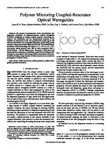


![Performance of Arrayed Microring Resonator ... - OMICS International [PDF]](https://m.moam.info/img/260x300/performance-of-arrayed-microring-resonator-omics-i_6479c46c098a9e9f088b4624.jpg)


