Numerical Simulation of Dynamic Flow Behaviour in a Bubble Column ...

Fourth International Conference on CFD in the Oil and Gas, Metallurgical & Process Industries SINTEF / NTNU Trondheim, Norway 6-8 June 2005

Numerical Simulation of Dynamic Flow Behaviour in a Bubble Column: Comparison of the Bubble-Induced Turbulence Models in the k-ε Model D. ZHANG, N.G. DEEN and J.A.M. KUIPERS University of Twente, Faculty of Science and Technology, P.O. Box 217, 7500 AE Enschede, Netherlands

ABSTRACT Numerical simulations of the gas-liquid bubbly flow in a bubble column were conducted with the commercial CFD package CFX-4.4 to investigate the performance of three models (Pfleger and Becker, 2001; Sato and Sekoguchi, 1975; Troshko and Hassan, 2001) to account for the bubble-induced turbulence in the k-ε model. Furthermore, the effect of two different interfacial closure models was investigated. All the predicted results were compared with experimental data. All three approaches could produce good solutions for the time-averaged velocity. The models of Troshko and Hassan (2001) and Pfleger and Becker (2001) resolve more details of the bubbly flow than the model of Sato and Sekoguchi (1975) does. In the top part of the column, the models of Troshko and Hassan and Pfleger and Becker under-predicts the liquid phase vertical velocity. Based on the comparison of the results for two columns of different aspect ratio (H/D = 3 and H/D = 6), it was found that the model of Pfleger and Becker (2001) performs better than the model of Troshko and Hassan (2001), while the model of Sato and Sekoguchi (1975) performs the worst. Furthermore, it was found that the interfacial closure model proposed by Tomiyama et al (2002) performs better for the tall column. NOMENCLATURE Ck model constant CD drag coefficient CL lift coefficient CVM virtual mass coefficient model constant Cε model constant Cε2 model constant Cε1 model constant Cμ Cμ ,BIT model constant d diameter D column depth E bubble aspect ratio Eo Eötvös number g acceleration of gravity H column height k turbulent kinetic energy

r M

p t

interface force vector pressure time

W

velocity vector column width

r U

α ε μ ρ σk σε τ

phase volume fraction turbulence dissipation rate dynamic viscosity density model constant model constant strain-stress tensor

Subscripts k phase indices rms root of mean square B bubble BIT bubble-induced turbulence D drag force G gas L liquid, lift force Lam Laminar Tur turbulent VM virtual mass force

INTRODUCTION Bubble column reactors are widely used in chemical, petrochemical and biochemical processes. The ability to predict fluid flow dynamics is of paramount importance in designing and developing bubble column reactors. Experimental investigation and numerical simulations are widely used to carry out predictions and analyse gas-liquid fluid flow process. Two approaches are mostly used to simulate the flow in bubble columns: the Euler-Euler (E-E) and EulerLagrange (E-L) approach. The E-L method is more suited for fundamental investigations of the bubbly flow while the E-E method is preferred in high gas hold-up and churn turbulent flows (Pan, Dudukovic and Chang, 1999). For both approaches, despite considerable efforts, accurate modelling of the two-phase turbulent Reynolds stress and interfacial forces remains an open question even for simple dispersed bubbly flow. In most work on gas-liquid two-phase flow, turbulence in the liquid phase is assumed as the sum of the shear and bubble-induced turbulence field and turbulence modelling is mostly done using a similar approach as for singlephase flow. Both k-ε and sub-grid scale (SGS) models are widely used in the simulation of the gas-liquid two-phase flow in the literature. Through a study of both the k-ε and sub-grid scale (SGS) models used in the simulation of

1

performance of this closure model in a numerical simulation is unclear. This work presents Euler-Euler three-dimensional dynamic simulations of gas-liquid bubbly flow in a square cross-sectioned bubble column. The differences among three different bubble-induced turbulence models proposed by Sato and Sekoguchi (1975), Pfleger and Becker (2001) and Troshko and Hassan (2001) are analysed in detail. Furthermore, the performance and applicability of Tomiyama’s interfacial force closures combined with the three bubble-induced turbulence models are investigated. All the numerical results are compared with experimental measurement data of Deen et al. (2001).

bubbly flow, Deen (2001) found that good agreement was obtained with the k-ε model in the simulation of the Becker case, while in the simulation of a threedimensional bubble column, the SGS model produces a better solution. When the k-ε model was employed to evaluate the turbulent viscosity, the bubble-induced turbulence is generally considered through two different approaches: Sato and Sekoguchi (1975) directly added an extra term to the effective viscosity. In the other approach, turbulence is taken into consideration for the liquid phase, the gas phase is modelled laminar but influences the turbulence in the liquid phase by a bubble-induced turbulence model (Johansen and Boysan, 1988; Oey, Mudde and Akker, 2003; Pfleger and Becker, 2001; Troshko and Hassan, 2001). That is, bubble-induced production terms are incorporated in the governing equations for k and ε. Several closure models for the bubble-induced production terms have been suggested (Johansen and Boysan, 1988; Kataoka and Serizawa, 1989; Lopez de Bertodano, Lahey and Jones, 1994, Pfleger and Becker, 2001; Troshko and Hassan, 2001), where the bubble-induced production in the governing equations of the liquid turbulent kinetic energy, k comes from the forces acting between a gas bubble and the surrounding liquid and the local slip velocity while the bubble-induced production in the liquid turbulence dissipation rate, ε equation is the result of the bubble-induced turbulence time scale,τBIT and the bubble-induced production in the k equation. The main difference among the mentioned bubble-induced turbulence models of the latter approach lies in the time scale of the bubble induced turbulence dissipation. In the model of Johansen and Boysan (1988) and Pfleger and Becker (2001), the smallest eddy time scale of the shear-induced turbulence was used as the characteristic time scale of the bubble-induced turbulence. Lopez de Bertodano (1992) found that when the shearinduced turbulence time scale is used as an estimate for the time scale of the bubble-induced turbulence, the turbulence decay depends on the initial dissipation rate, which is unphysical. For this reason they proposed a new expression for the bubble-induced turbulence time scale, which is determined by the bubble residence time. Troshko and Hassan (2001) adopted this time scale. In the simulations of Johansen and Boysan (1988) and Pfleger and Becker (2001) and Troshko and Hassan (2001), numerical results fit well with the experiments, though the time scale used to calculate the bubble-induced turbulence production in the liquid phase turbulence dissipation rate equation are quite different. Though all the models could provide good solutions for the time-averaged velocities, to the best of our knowledge, the validity of the predicted sub-grid scale quantities is not clear, nor is the difference between these models. In this work, the performance of these two models, along with the model of Sato and Sekoguchi was investigated for the case of a square crosssectioned bubble column. The bubble drag, lift and virtual mass coefficients, CD, CL, CVM used in the interfacial closure model are of great importance in numerical simulation of bubbly flows. Despite considerable efforts (Clift, Grace and Weber, 1978, Magnaudet, Eames, 2000), accurate modelling of the interfacial forces remains an open question in numerical simulations. Recently, Tomiyama (2004) proposed a set of closures for these three coefficients based on a large experimental data set. However, the

PHYSICAL PROBLEM A schematic representation of the bubble columns used in this report is shown in Figure 1. The whole column is filled with water, which acts as the continuous liquid phase. Air was used as the dispersed gas phase and was injected in the centre of the bottom plane with Ain = 0.03 × 0.03 m2 and a superficial gas velocity of VS = 4.9 mm/s. The gas-liquid flow is assumed to be homogeneous (bubbly) flow. Consequently, break-up and coalescence are not accounted for. The column has the following dimensions: width (W) 0.15 m, depth (D) 0.15 m and height (H) 0.45 or 0.90 m. All the simulation parameters and physical properties are presented in Table 3. Numerical simulations were conducted with the commercial CFD package CFX-4.4 of AEA Technology, Harwell, UK. The numerical simulations are compared with experimental data of Deen et al. (2001).

H = 0.45 m or 0.90 m

y,v

m

0.06 m

z,w

0. = W

0. 06

m

15

0.06 m

0.

06

m

x,u

D = 0.15 m

Figure 1: Schematic representation of the investigated bubble columns. GOVERNING EQUATIONS The equations of the two-fluid formulation are derived by ensemble averaging the local instantaneous equations of single-phase flow (Drew, 1999). Two sets of balance equations for mass and momentum are obtained. Ignoring the interfacial mass transfer, the generic conservation equations for mass and momentum respectively take the following form:

2

r ∂ (α k ρ k ) + ∇ ⋅ (α kU k ) = 0 ∂t r r r ∂ (α k ρ kU k ) + ∇ ⋅ (α k ρ kU kU k + α kτ k ) = ∂t r r α k ρ k g − α k ∇pk + M k

referred to as pseudo-turbulence or bubble-induced turbulence. In this work we use two models to account for the bubble-induced turbulence. One is to use the standard k - ε model, i.e., Sk,BIT and Sε,BIT in Eq.6 and Eq.7 are set to zero. In that case, the bubble-induced turbulence is accounted for through the effective viscosity, μeff. Another approach to account for the bubble-induced turbulence is to include extra source terms in the turbulent models, that is, the bubble-induced turbulence is implicitly included in Eq.5. When the former model is used, the model proposed by Sato and Sekoguchi (1975) was used to account for the bubble-induced turbulence in Eq.4:

(1)

(2)

where the indices k refers to the phase (L for liquid, G for gas). The volume fraction of each phase is denoted by α

r r r r U = ui + vj + wk is the velocity vector. For phase k, the stress-strain tensor τ k is given by: r r r 2 (3) τ k = − μ eff (∇U k + (∇U k )T − I ∇ ⋅ U k ) 3 and

r

When the bubble-induced turbulence is accounted for in Eqs. 6 and 7, μBIT is set to zero. As mentioned earlier, the source terms suggested by Pfleger and Becker (2001) and Troshko and Hassan (2001) are selected to account for the bubble-induced turbulence. All the three bubble-induced turbulence models are summarized in Table 1.

In this paper, the k- ε model is employed to evaluate the liquid phase turbulent viscosity; the gas phase is modelled laminar but influences the turbulence in the liquid phase through a bubble-induced turbulence model. The turbulent viscosity of the liquid phase is calculated by:

kL

r

The term M k in Eq.2, describes the interface forces, which are given as follows:

r r r r r M tot , L = − M tot ,G = M D , L + M L , L + M VM , L

2

The conservation equations for k and ε are respectively given by

r ∂ (α L ρ L k L ) + ∇ ⋅ (α L ρ LU L k L − α L ( μ Lam, L ∂t

r r r r 3 C r M D , L = α G ρ L D | U G − U L | (U G − U L ) (10) dB 4 r r r r (11) M L , L = α G ρ L CL (U G − U L ) × ∇ × U L r r r DU DU (12) M VM , L = α G ρ LCVM ⋅ ( G G − L L ) Dt Dt

(6)

μ + Tur , L )∇k L ) = α L (GL − ρ Lε L ) + Sk , BIT σk ∂ (α L ρ Lε L )

According to Tomiyama (2004), the virtual mass coefficient CVM for a spherical bubble in potential flow and in a Stokes flow is known to be 0.5. For a spheroidal bubble, CVM is no longer a scalar but is a tensor:

+

∂t

r μ ∇ ⋅ (α L ρ LU Lε L − α L ( μ Lam, L + Tur , L )∇ε L )

σε

= αL

εL kL

(7)

CVM

(Cε 1GL − Cε 2 ρ Lε L ) + Sε , BIT

Source

h ⎛ CVM ⎜ =⎜ 0 ⎜ 0 ⎝

0 v CVM 0

0 0 h CVM

⎞ ⎟ ⎟ ⎟ ⎠

(13)

h v is the horizontal component and CVM is the where CVM

with Ck = Cε1 = 1.44, Cε = Cε2 = 1.92, Cμ = 0.09, σk = 1.0 and σε = 1.217. It is noted that these constants are not universal even in the case of single-phase flow. For multiphase flows they are still under debate. The vorticity generated in the wake of the bubbles is often

vertical component. In the approach of Pfleger and Becker (2001),

r r r | M tot | ⋅ | U G − U L | represents the energy input of the

Sk,BIT

Sε,BIT

μBIT

0

0

Eq.8

BIT Model 1 (Sato and Sekoguchi ,1975) 2 (Pfleger and Becker, 2001) 3 (Troshko and Hassan, 2001)

(9)

where the terms on the right hand side represent forces due to drag, lift and virtual mass, respectively. The forces are respectively calculated as:

(5)

εL

(8)

where Cμ ,BIT is a model constant, which is set to 0.6.

The effective viscosity of the liquid phase,μL,eff is composed of three contributions: the molecular viscosity μL,Lam, the turbulent viscosity μL,Tur and an optional term due to bubble induced turbulence μBIT : (4) μ L ,eff = μ L , Lam + μ L ,Tur + μ BIT

μ L ,Tur = Cμ ρ L

r

μ BIT = ρ Lα G Cμ , BIT d B | U G − U L |

r

r

r

α LCk | M tot | ⋅ | U G − U L | r r r | M D,L | ⋅ | U G − U L |

εL kL

Cε S k , BIT

r r 3CD | U G − U L | 0.45 S k , BIT 2CVM d

Table 1: Three different models for bubble-induced turbulence in bubbly flow.

3

0

Closure model A

Closure model B (Tomiyama, 2004)

8 Eo(1 − E 2 ) F ( E ) −2 3 E 2 / 3 Eo + 16(1 − E 2 ) E 4 / 3 1 (Wellek et al. ,1966) E= 1 + 0.163Eo 0.757 sin −1 1 − E 2 − E 1 − E 2 F (E) = 1− E2 CD =

CD =

2 Eo 3

(Ishii-Zuber, 1979)

⎧min[0.288 tanh(0.121Re), f ( Eod )] Eod < 4 CL = ⎨ Eod ≥ 4 ⎩ f ( Eod ) 2/3 Eod = Eo / E

CL = 0.5

f ( Eod ) = 0.00105 Eod3 − 0.0159 Eod2 − 0.0204 Eod + 0.474 h CVM =

h CVM = 0.5 v VM

C

= 0.5 v CVM =

E cos −1 E − 1 − E 2 E 2 1 − E 2 − E cos −1 E cos −1 E − E 1 − E 2 (2 E −1 − E ) 1 − E 2 − cos −1 E

Table 2: Investigated interfacial force closures.

The total domain is subdivided into uniform computational grid cells with Δx = Δy = Δz = 0.01 m, which proved to have a sufficient resolution (Deen et. al., 2001). Eqs. (1), (2), (6) and (7) were solved in a transient fashion with a fully implicit backward Euler differencing scheme with a time step of 0.005 s. The curvature compensated convective transport (CCCT) scheme was used for all convective terms in the momentum equations. All the presented results are time-averaged quantities, which were selected in a plane at z/W = 0.50. The simulation parameters for all test cases are presented in Table 3.

bubbles resulting from the forces acting between the turbulence, τ BIT = ε L / k L to represent the time scale for the dissipation of the bubble-induced turbulence. Whereas Troshko and Hassan (2001) assume that the characteristic time scale of bubble-induced turbulence is determined by the bubble response time, which takes the form

r

r

τ BIT = 3CD | U G − U L | /(2CVM d B ) .

In this paper, two

sets of interfacial force closures are used; these are listed in Table 2. In all simulations, a pressure boundary condition was used at the outlet. No-slip conditions were used at the walls.

Case

BIT model

1A3

1

2A3

2

3A3

3

1B3

1

2B3

2

3B3

3

1A6

1

2A6

2

3A6

3

1B6

1

2B6

2

3B6

3

Interfacial force closure

H/D

A 3 B

A 6 B

ρL = 1000 kg/m3, μL = 0.001 kg/(m.s), σ = 0.073 N/m, dB = 4 mm ρG = 1.29 kg/m3, μG = 1.8×10-5 kg/(m.s), Eo = 2.2, Eod = 2.6 Table 3: Simulation and case parameters.

4

0.20

DATA PROCESSING In order to compare the numerical results with the experimental data, the time-averaged quantities are calculated as defined in the following expressions. The time-averaged mean velocity is calculated as:

n − n0 − 1 1 un −1 + un n − n0 n − n0

(15)

where the averaging is started at time step n0 = 7500, corresponding to 37.50 s. All simulations were carried out for n = 105, corresponding to a period of 500 s. The large-scale velocity fluctuations are calculated during the calculation as follows: 2 2 urms , n = un − un

2

0.10

vm,L (m/s)

un =

0.15

Case 1A3 Case 2A3 Case 3A3 exp. (y/H=0.50)

0.05

0.00

-0.05 0.0

0.2

0.4

0.6

0.8

1.0

0.8

1.0

0.8

1.0

0.8

1.0

x/D (-)

(16)

0.4

RESULTS AND DISCUSSION Three different approaches to account for the bubbleinduced turbulence in the k-ε turbulence model are studied (see Table 1). Furthermore, two different interfacial closure models (see Table 2) and two different columns were investigated. All cases are summarized in Table 3, where the case number indicates the bubbleinduced turbulence model, the interfacial closure model and the aspect ratio of the column. The performance and capacity of three different bubble-induced turbulence models will be discussed first, subsequently, the applicability of Tomiyama’s interfacial closures in simulation of the bubbly flows will be evaluated. Finally, the performance of the best model will be assessed for a column with H/D = 6.

vm,G (m/s)

0.3

Case 1A3 Case 2A3 Case 3A3 exp. (y/H=0.50)

0.2

0.1

0.0 0.0

0.2

0.4

0.6 x/D (-)

0.20

0.15 vm,L (m/s)

The effect of the bubble-induced turbulence model

0.10

Figure 2 presents the time-averaged vertical velocity profiles at two different heights for cases 1A3, 2A3 and 3A3. In the lower part of the column (y/H < 0.50), the predicted results agree well with the experimental data. But with increasing height, the numerical results of case 2A3 and 3A3 slightly under-predict the experimental data for the liquid phase, but still fit well with the experimental data for the gas phase. It is clearly shown in this figure that the vertical velocity profiles obtained from the Sato and Sekoguchi (1975) model (Case 1A3) is higher than in the other two cases. This is due to the fact that Sato and Sekoguchi’s model yields a higher effective liquid viscosity. Consequently as is shown in Figure 3, the simulated velocity fluctuations are less than in the experimental data whereas the models of Troshko and Hassan (2001) and Pfleger and Becker (2001) produce a good solution for the velocity fluctuations. Figure 4 shows the turbulent quantity distributions obtained from the different bubble-induced turbulence models. In the model of Sato and Sekoguchi less of the dynamics of the flow are resolved, instead they are implicitly included in the turbulent kinetic energy. Compared with the model of Pfleger and Becker, the model of Troshko and Hassan seems to resolve more of the dynamics of the flow, that is, more liquid velocity fluctuations are captured instead of implicitly contained in the turbulence model. The time scale of the shear-induced turbulence is also provided in Figure 4(b). The time scale of the bubble-induced turbulence, according to Lopez de Bertodano (1992), r r τ BIT = 2CVM d B /(3CD | U G − U L |) , is about 0.006 s

Case 1A3 Case 2A3 Case 3A3 exp. (y/H=0.63)

0.05

0.00

-0.05 0.0

0.2

0.4

0.6 x/D (-)

0.4

vm,G (m/s)

0.3

0.2

Case 1A3 Case 2A3 Case 3A3 exp. (y/H=0.63)

0.1

0.0 0.0

0.2

0.4

0.6 x/D (-)

Figure 2: Comparison of the simulated time-averaged vertical velocity profiles of both phases with the experimental data using different bubble-induced turbulence models to account for the bubble-induced turbulence.

5

0.11 0.10

for all three cases in the current simulations. This time scale is much smaller than the time scale of the smallest eddy dissipation in the liquid phase, which means that the bubble-induced turbulence is dissipated much faster than shear-induced turbulence in this bubbly flow.

0.09

uL,rms (m/s)

0.08 0.07

Case 1A3 Case 2A3 Case 3A3 exp. (y/H=0.63)

0.06 0.05 0.04

The effect of the interfacial closure model

Tomiyama’s interfacial closures (2004) are tested with the help of cases 1B3, 2B3 and 3B3. Figure 5 shows the timeaveraged vertical velocity profiles for both phases. For the model of Pfleger and Becker (2001) and Troshko and Hassan (2002), a relatively steep velocity profile is found. This can be attributed to the lift force, which disperses the bubble plume towards the side walls. In the model of Tomiyama, CL is relatively small (CL ≈ 0.3) compared to the CL = 0.5 in case A. Consequently, the bubble plume is not sufficiently dispersed, which leads to a relatively steep velocity profile. Figure 6 shows the liquid phase velocity fluctuation distributions in vertical and horizontal directions. The model of Sato and Sekoguchi (1975) in combination with Tomiyama’s interfacial force closures leads to an almost stationary bubble plume. With a smaller CL the plume is less dynamic in the horizontal direction while in the vertical direction, the plume is much more dynamic in the column centre.

0.03 0.02 0.01 0.00 0.0

0.2

0.4

0.6

0.8

1.0

x/D 0.20

vL,rms (m/s)

0.15 Case 1A3 Case 2A3 Case 3A3 exp. (y/H=0.63)

0.10

0.05

0.00 0.0

0.2

0.4

0.6

0.8

The effect of the column aspect ratio

1.0

In the above simulations, it was found that interfacial closure model A performs better for the simulation of bubbly flow in the bubble column with H/D = 3. In order to assess their prediction capability, the best models were also used to simulate the flow in a taller column (H/D = 6).

x/D (-)

Figure 3: Time-averaged plot of the vertical and horizontal velocity fluctuations of the liquid phase with different bubble-induced turbulence models.

0.020

0.3

0.015

0.2

2

2

kL,sgs (m /s )

0.025

0.010

0.005

0.000 0.0

0.2

0.4

0.6

vm,L (m/s)

Case 1A3 Case 2A3 Case 3A3 (y/H = 0.63)

0.8

1.0

(a)

0.0

0.8

0.2

0.4

0.6 x/D (-)

0.8

1.0

0.8

1.0

0.5

0.6

0.4 Case 1A3 Case 2A3 Case 3A3 (y/H = 0.63)

0.4

vm,G (m/s)

kL,sgs/εL,sgs (s)

Case 1B3 Case 2B3 Case 3B3 exp. (y/H=0.57)

0.0

-0.1

x/D (-)

0.2

0.0 0.0

0.1

0.3

0.2

Case 1B3 Case 2B3 Case 3B3 exp. (y/H=0.57)

0.1

0.2

0.4

0.6

0.8

1.0

x/D (-)

0.0 0.0

(b) Figure 4: Time-averaged liquid phase distributions of turbulent quantities with different bubble-induced turbulence models: (a) turbulent kinetic energy; (b) time scale of the shear-induced turbulence.

0.2

0.4

0.6 x/D (-)

Figure 5: Comparison of the simulated time-averaged vertical velocity profiles of both phases obtained with Tomiyama’s interfacial closures and experimental data.

6

0.4 0.10

0.3 vm,G (m/s)

uL,rms (m/s)

0.08

0.06

0.2

Case 1B3 Case 2B3 Case 3B3 exp. (y/H=0.57)

0.04

Case 1A6 Case 2A6 Case 3A6 exp. (y/H=0.57)

0.1

0.02

0.00 0.0

0.0 0.0 0.2

0.4

0.6

0.8

0.2

0.4

0.6

0.8

1.0

x/D (-)

1.0

x/D (-)

0.15

0.35

vL,rms (m/s)

0.25

Case 1B3 Case 2B3 Case 3B3 exp. (y/H=0.57)

0.10 vm,L (m/s)

0.30

0.20

0.05

0.15 0.10 0.05 0.00 0.0

Case 1A6 Case 2A6 Case 3A6 exp. (y/H=0.57)

0.00

-0.05 0.0 0.2

0.4

0.6

0.8

0.2

0.4

0.6

0.8

1.0

0.8

1.0

x/D (-)

1.0

x/D (-)

0.15

Figure 6: Time-averaged plot of the vertical and horizontal velocity fluctuations of the liquid phase obtained with Tomiyama’s interfacial force closures. vm,L (m/s)

0.10

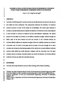
Figure 7 shows the time-averaged vertical velocity profiles for both phases with three different bubbleinduced turbulence models. None of the three bubbleinduced turbulence models can provide a good solution for both phases simultaneously. For this reason, the same system was also simulated with model B. Figure 8 shows the time-averaged vertical velocity profiles for both phases at two different heights. The predicted gas phase vertical velocities agree rather well with the experimental data, but the simulated liquid phase vertical velocity profiles are lower than in the experiments. Maybe this is due to the fact, that we treat the outlet boundary as a rigid plane, while in reality, the outlet is a dynamic free surface. This free surface dominates the flow structure in the top of the column in such way that the bubble plume is not spread throughout the column, as is the case in the simulation. Figure 9 shows the snapshots of the instantaneous iso-surface of αG = 0.01 and liquid velocity field after 500 s for different bubble-induced turbulence models and interfacial closure models. Clearly, it is found that compared with interfacial closure A, Tomiyama’s interfacial models increase the height where the bubble plume is spread throughout the column. Furthermore, compared with the models of Pfleger and Becker (2001) and Troshko and Hassan (2002), it can be seen in these snapshots that the model of Sato and Sekoguchi (1975) provides a quasi-steady state plume and does not resolve more small structures or the details of the bubbly flow. In this column, it seems that the model of Pfleger and Becker resolves slightly more details of the bubbly flow than that of Troshko and Hassan. Figure 10 shows a comparison of

Case 1A6 Case 2A6 Case 3A6 exp. (y/H=0.73)

0.05

0.00

-0.05 0.0

0.2

0.4

0.6 x/D (-)

0.4

vm,G (m/s)

0.3

0.2 Case 1A6 Case 2A6 Case 3A6 exp. (y/H=0.73)

0.1

0.0 0.0

0.2

0.4

0.6

0.8

1.0

x/D (-)

Figure 7: Comparison of the simulated time-averaged vertical velocity profiles of both phases and experimental data.

7

vertical directions. As indicated in Figure 9, most transient details are not resolved by the model of Sato and Sekoguchi, the predicted velocity fluctuations obtained from their model are lower than the experimental profiles. Again, as found in Figure 6, the velocity fluctuations in the vertical direction are much stronger than in the horizontal direction. The model of Troshko and Hassan predicts the velocity fluctuation in the horizontal slightly better than that of Pfleger and Becker, but in the vertical direction, the difference is quite small. Combining the information of Figure 8 and 10, it can also be concluded that the bubble-induced turbulence model proposed by Pfleger and Becker performs better than that of Troshko and Hassan. This is opposite to the observation that was made for the low column. The reason for this discrepancy is currently not explained. In future work, we plan to address the modelling of the free surface.

0.20

vm,L (m/s)

0.15 0.10 0.05 Case 1B6 Case 2B6 Case 3B6 exp. (y/H=0.57)

0.00 -0.05 0.0

0.2

0.4

0.6

0.8

1.0

0.8

1.0

x/D (-)

0.40 0.35

vm,G (m/s)

0.30 0.25 0.20 Case 1B6 Case 2B6 Case 3B6 exp. (y/H=0.57)

0.15 0.10 0.05 0.00 0.0

0.2

0.4

0.6 x/D (-)

0.20

vm,L (m/s)

0.15

0.10

Case 1A6

Case 2A6

Case 3A6

Case 1B6

Case 2B6

Case 3B6

0.05 Case 1B6 Case 2B6 Case 3B6 exp. (y/H = 0.73)

0.00

-0.05 0.0

0.2

0.4

0.6

0.8

1.0

x/D (-) 0.4

vm,G (m/s)

0.3

0.2 Case 1B6 Case 2B6 Case 3B6 exp. (y/H = 0.73)

0.1

0.0 0.0

0.2

0.4

0.6

0.8

1.0

x/D (-)

Figure 8: Comparison of the simulated time-averaged vertical velocity profiles of both phases and experimental data.

Figure 9: Snapshots of the instantaneous iso-surface of αG = 0.01 and liquid velocity field after 500 s for different bubble-induced turbulence models and interfacial closure models.

the simulated and experimental profiles of the timeaveraged liquid velocity fluctuations in the horizontal and

8

0.12

Case 1B6 Case 2B6 Case 3B6 exp. (y/H=0.57)

0.10 urms,L (m/s)

(H/D = 6) Tomiyama’s interfacial force closures produce a quite good solution. With a higher value for CD and smaller value for CL, Tomiyama’s interfacial force closures increase the height where the bubble plume is spread out to the full column. Further work is still needed to obtain a good solution for the liquid phase velocity in the top portion of the taller column.

0.08 0.06

REFERENCES CLIFT, R., GRACE, J.R. and WEBER, M.E., (1978) “Bubbles, Drops, and Particles”, Academic Press. New York. DEEN, N.G., SOLBERG, T., and HJERTAGER, B.H., (2001) “Large eddy simulation of the Gas-Liquid flow in a square cross-sectioned bubble column”, Chem. Eng. Sci., 56, 6341-6349. ISHII, M. and ZUBER, N., (1979) “Drag coefficient and relative velocity in bubbly, droplet or particulate flows”, AIChE J., 25, 843-855. JOHANSEN, S. T. and BOYSAN, F., (1979) “Fluid dynamics in bubble stirred ladles: Part II. Mathematical modelling”, MET. TRANS. B, 19, 755-764. KATAOKA, I. and SERIZAWA, A., (1989) “Basic equations of turbulence in gas-liquid two-phase flow”, Int. J. Multiphase Flow, 15, 843-855. MAGNAUDET, J. and EAMES, I., (2000) “The Motion of High-Reynolds Number Bubbles in inhomogeneous Flows”, Ann. Rev. Fluid Mech., 32, 659-708. LOPEZ DE BERTODANO, M.A., (1992) “Turbulent bubbly two-phase flow in a triangular duct”, Ph.D dissertation, Rensselaer Polytechnic Institute. LOPEZ DE BERTODANO, M.A., LAHEY, R.T. and JONES, O.C., (1994) “Development of a k-ε model for bubbly two-phase flow”, J. Fluids Eng., 116, 128-134. OEY, R.S., MUDDE, R.F., and VAN DEN AKKER, H.E.A.., (2003) “Sensitivity study on interfacial closure laws in two-fluid bubbly flow simulations”, AIChE J., 49, 1621-1636. PAN, Y., DUDUKOVIC, M.P. and CHANG, M., (1999) “Dynamic simulation of bubbly flow in bubble columns”, Chem. Eng. Sci., 54, 2481-2489. PFLEGER, D. and BECKER, S., (2001) “Modeling and simulation of the dynamic flow behavior in a bubble column”, Chem. Eng. Sci., 56, 1737-1747. SATO, Y. and SEKOGUCHI, K., (1975) “Liquid velocity distribution in two-phase bubble flow”, Int. J. Multiphase Flow, 2, 79-95. TOMIYAMA, A., (2004) “Drag, lift and virtual mass forces acting on a single bubble”, 3rd International Symposium on Two-Phase Flow Modeling and Experimentation. Pisa, Italy. 22-24 Sept. TROSHKO, A.A. and HASSAN, Y.A., (2001) “A twoequation turbulence model of turbulent bubbly flows”, Int. J. Multiphase Flow, 27, 1965-2000. WELLEK, R.M., AGRAWAL, A.K. and SKELLAND, A.H.P., (1966) “Shape of liquid drops moving in liquid media”, AIChE J., 12, 854–862.

0.04 0.02 0.00 0.0

0.2

0.4

0.6

0.8

1.0

x/D (-) 0.25 Case 1B6 Case 2B6 Case 3B6 exp. (y/H=0.57)

vrms,L (m/s)

0.20

0.15

0.10

0.05

0.00 0.0

0.2

0.4

0.6

0.8

1.0

x/D (-)

Figure 10: Comparison of the simulated and experimental profiles of the time-averaged liquid velocity fluctuations in the horizontal and vertical directions in a column with H/D = 6.

CONCLUSIONS Numerical simulations of the gas-liquid two-phase flow in a square cross-sectioned bubble column were conducted with the use of the commercial software package CFX-4.4. The k-ε model was employed to model the turbulent viscosity of the liquid phase. The difference between three different models to account for the bubble-induce turbulence was studied. The simulated velocity fluctuations for the liquid phase predicted with the models of Troshko and Hassan (2001) and Pfleger and Becker (2001) satisfy well with the measurements. In the Sato and Sekoguchi (1975) model, most of the transient details of the bubbly flow are implicitly contained in the sub-grid scale turbulence kinetic energy, kL,sgs. Consequently this leads to a quasi-steady state while the model of Pfleger and Becker (2001) and Troshko and Hassan (2001) can resolve most transient details of the bubbly flow. The model of Sato and Sekoguchi (1975) leads to a higher turbulent viscosity and only resolves the overall flow pattern. The models of Pfleger and Becker, and Troshko and Hassan can provide a good solution for the gas phase vertical velocity, but under-predict the liquid phase vertical velocity in the top part of the column. Based on all simulations, the model of Pfleger and Becker performs slightly better than that of Troshko and Hassan. Though simulated results obtained from Tomiyama’s interfacial force closures do not satisfy the experimental data in the lower bubble column (H/D = 3), in a taller column

9