Numerical Simulation of Pore-Scale Flow in

THEORETICAL & APPLIED MECHANICS LETTERS 1, 022008 (2011)

Numerical simulation of pore-scale flow in chemical flooding process Xiaobo Li,1, a) Shuhong Wu,1 Jie Song,1 Hua Li,1 and Shuping Wang2 1) 2)

Research Institute of Petroleum Exploration & Development of Petrochina, Beijing 100083, China Petroleum Exploration & Production Research Institute of Sinopec, Beijing 100083, China

(Received 11 January 2011; accepted 26 January 2011; published online 10 March 2011) Abstract Chemical flooding is one of the effective technologies to increase oil recovery of petroleum reservoirs after water flooding. Above the scale of representative elementary volume (REV), phenomenological modeling and numerical simulations of chemical flooding have been reported in literatures, but the studies alike are rarely conducted at the pore-scale, at which the effects of physicochemical hydrodynamics are hardly resolved either by experimental observations or by traditional continuum-based simulations. In this paper, dissipative particle dynamics (DPD), one of mesoscopic fluid particle methods, is introduced to simulate the pore-scale flow in chemical flooding processes. The theoretical background, mathematical formulation and numerical approach of DPD are presented. The plane Poiseuille flow is used to illustrate the accuracy of the DPD simulation, and then the processes of polymer flooding through an oil-wet throat and a water-wet throat are studies, respectively. The selected parameters of those simulations are given in details. These preliminary results show the potential of this novel method for modeling the physicochemical hydrodynamics c 2011 The Chinese Society of at the pore scale in the area of chemical enhanced oil recovery. ⃝ Theoretical and Applied Mechanics. [doi:10.1063/2.1102208] Keywords chemical flooding, pore-scale flow, dissipative particle dynamics, mesoscopic simulation, enhanced oil recovery Chemical flooding, among the various enhanced oil recovery (EOR) techniques, is playing a dominating role in China.1 The EOR mechanism of chemical flooding is that addition of some chemical agents (e.g. alkaline, polymer, surfactant) to injected water makes higher sweep efficiency and/or oil-displacement efficiency. As the chemical EOR technique develops for some oil reservoirs with low primary and water-flooding oil recovery, some aspects of this technology need further studies. One of the research focusing on chemical EOR lies on how to evaluate the possible performance of oildisplacement agents in reservoir. Above representative elementary volume (REV), the phenomenological model formulation and numerical solution of chemical flooding have been reported in some papers,2 and the distribution of oil saturation and pressure in reservoir can be given by numerical simulations of chemical flooding. Most of the phenomenological parameters in chemical EOR models need to be obtained by laboratory experiments. To maximize the application potential of chemical flooding and explore the potential high-performance chemical agents, the phenomena at the pore-scale must be studied. Both physicochemical and hydrodynamic effects are of great importance at the pore scale (∼ µm), which can hardly be resolved by experimental studies. Some novel theoretical models and numerical simulation approaches should be searched for. A bottom-up approach to model the fluid flow through porous media is displayed in Fig. 1. The continuum-based approaches modelling the macroscopic a) Corresponding

author. Email: [email protected].

Fig. 1. The bottom-up approach to model the fluid flow through porous media

phenomena ignore fully the microscopic effects. Microscopic molecular dynamics, on the other hand, requires excessive times and efforts before the macroscopic effects become meaningful or make sense. It’s feasible to study the pore-scale flow in chemical flooding process by mesoscopic (between micro- and macro-) methods. Three of popular mesoscopic methods are Lattice Boltzmann method (LBM), smoothed particle hydrodynamics (SPH) and dissipative particle dynamics (DPD).3 LBM can be regarded as the numerical realization of generalized Boltzmann equation, and SPH is the Lagrangian formulation of macroscopic fluid dynamics on integral interpolants. LBM and SPH are mostly used by the researchers who are focussed more on the hydrodynamics phenomena than on physicochemical ones. In the area of chemical EOR, some physicochemical phenomena (e.g. wettability) are essential for industrial

022008-2 X. Li, S. Wu, J. Song, H. Li, and S. Wang

Theor. Appl. Mech. Lett. 1, 022008 (2011)

applications. Besides, there are two advantages of DPD as follows. rˆi (t + ∆t) = rˆi (t) + ∆tˆ vi (t) + 21 ∆t2 Fˆi (t), (1) Compared with LBM, the non-lattice DPD method provides more flexible treatment of complex solid boundary in porous. (2) Owing to the same numerical formulation as used in molecular dynamics (MD), DPD method has the potential to establish a multi-scale simulation architecture. In the model of DPD,4–6 the fluid is represented with discrete beads, and each one corresponds to a cluster (the number is Nm ) of real molecules or radicals. The beads interact with each other via pair-wise conservation, random, and dissipative forces that locally conserve momentum leading to a correct hydrodynamic description. In our simulation, the cut-off radius rc and the mass of one DPD beads mDPD were respectively chosen as the characteristic length and mass, and the imposed flow rate U is chosen as the characteristic flow rate. The force exerted on each bead is given as

vˆi′ (t + ∆t) = vˆi (t) + λ∆tFˆi (t), Fˆi (t + ∆t) = Fˆi [ˆ ri (t + ∆t) , vˆi′ (t + ∆t)], [ ] vˆi (t + ∆t) = vˆi (t) + 21 ∆t Fˆi (t) + Fˆi (t + ∆t) , (3) where λ is the integration parameter, and the value is chosen as 0.65 in our simulation. The selection of the parameters for DPD simulation is the main topic in several DPD studies.5,7,8 The transport properties of a DPD fluid can be obtained as measurable quantities resulting from a chosen set of DPD input parameters. According to the proposed relation for the viscosity of DPD fluid,9 the factor of dissipative force can been given as γˆ ≈

1 575 1 ˆ ×n 2π Re ˆ DPD

(4)

(1)

To determine the proper value of conservative force coefficient α, a reported relationship between the mesoscopic model parameter and the compressibility of the system is give5 ( ) 1 nDPD κ ˆ= 1 + 2α (5) Nm kb T

where vˆij , rˆij and eij are the dimensionless relative velocity, the distance and unit vector between bead i and bead j, respectively. α ˆ is the conservative factor, which is the maximum repulsive force between two beads, and γˆ are the dissipative factor. The random variable ξij is selected from a Gaussian distribution with zero mean and unit variance, and ∆tˆ is the time step. The apparent Peclet number Pˆ e is the ratio of the characteristic flow rate U to the thermal velocity of the system, UT . Both the thermal and hydrodynamic effects of fluid system exist at the pore scale, and high value of Pˆ e means that the hydrodynamic actions dominate in determining the movement of fluid beads. w ˆ D and w ˆ R are the dissipation and the fluctuation weight function, one of which can be chosen arbitrarily and the choice fixes the other function. A generalized form of weight function is usually given by

The value of the conservative force parameter α can be determined from Eq. (5) by referring to the isothermal compressibility of fluid κ ˆ . Both experimental measurements and molecular dynamics (MD) simulations can be used to determine the value of κ ˆ , and the latter provides a probable multi-scale simulation approach to relate the molecular behavior of chemical agents and its oil-displacement effects. Some literatures in the area of physical-chemical research have shown the feasibility of the above-mentioned approach,5 but the problem to determine the value of conservative force coefficient α are not completely solved. The value of α keeps linear relationship with the value of Nm in Eq. (5) for a fixedˆ κ, which is not correct if Nm takes a very larger value (usually for the simulation of hydrodynamic phenomena). For most of DPD simulations of water (ˆ κ ∼16), the influence of coarse-graining parameter Nm is ignored, and Eq. (6) is often simplified into the following form

Fˆi =

∑

[ α ˆ (1 − rˆij ) − γˆ w ˆ D (ˆ eij · vˆij )+

j̸=i 1

ˆ R ξij γˆ 2 w √ + Pˆ e ∆tˆ

] · eˆij

[ R ]2 2 = (1 − rˆij ) . w ˆD = w ˆ

(2)

The procedure of DPD simulation is the same as used in molecular dynamics simulation, and the movement of each DPD bead satisifies the classical Newtonian law. A modified version of the velocity-verlet algorithm is used to integrate the equations of motion.5 The evolution of positions and velocities of beads is determined as follows

α ˆ=

75 2×n ˆ DPD × Pˆ e2

.

(6)

By the fluctuation-dissipation theorem, there is a relation between the factor of dissipative force γˆ and the factor of random force σ ˆ .6 / 1 2 Pˆ e. (7) σ ˆ = γˆ

022008-3 Numerical simulation of pore-scale flow

To check the accuracy of the DPD simulation and illustrate the selection of its parameters, a plane Poiseuille flow, the steady state flow between two stationary parallel plates, is studied here. The analytical solution of this flow model can be derived from continuum-based Navier-Stokes equations, where the flow has a parabolic-like velocity profile. In this simulation, only one kind of beads is used to represent the fluid of water, and the viscosity of the fluid is 0.523 mPa · s. The simulation scale is set as 10rc × 20rc × 10rc , and the number of total beads is 8 000. Each bead represents a cluster of 2 × 107 real molecules. The relations between measurable physical quantities of fluid and DPD parameter are given in Appendix 1, and the values of parameters used in our simulation are chosen as follows: the coarse-graining number is 2 × 107 , the bead number density is 4, the cut-off radius is about 1.337 × 10−7 m, the characteristic velocity is 0.246 m/s, the conservative force factor is 2.349, and the dissipative force factor is 994.716. The method of periodic Poiseuille flow is adopted to eliminate the drawbacks of artificial solid wall,10 where a mass force with the value of (1.905) acts on each bead, and the direction of the force is negative when 0 < y < 10 and is positive when 10 < y < 20 (Fig. 2). The periodic boundary conditions are used at x-, y- and z- axis.

Theor. Appl. Mech. Lett. 1, 022008 (2011)

Fig. 3. The result of DPD simulation for the periodic Poiseuille flow

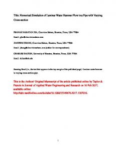
Following the traditional continuum-based approach, some specific constitutive relations for the EOR fluids must beestablished, and the evolution of interface between different fluid phases needs to be captured. For DPD method, the above-mentioned challenges can be conveniently dealt with due to intrinsic advantages of fluid particle methods (FPM). In this simulation, four kinds of DPD beads are used to represent polymer, water, oil and solid wall, denoted respectively by P, W, O and S. The polymer macromolecules are constructed by connecting several DPD beads together with nonlinear springs, and the number of beads in one macromolecular is 10. Spring force Fˆ sij is calculated by the finite extensible nonlinear elastic (FENE) model11 Fˆ si,j = −

Fig. 2. Illustration of the periodic Poiseuille flow

The simulation result is shown in Fig. 3. As a whole, the velocity profile simulated with DPD is in good agreement with the analytical solution of N-S equations. The fluctuation of velocity in DPD simulation reflects the stochastic property of flows under the condition of low Pˆ e number (1.998).

kˆs × rˆij 1 − (ˆ rij /ˆ rm )

2

· eˆij

(8)

where kˆs and rˆm are the spring force factor and the maximum permissible length of one chain segment, respectively, which are set as kˆs = 6 and rˆm = 3 in this simulation. The spring force increases drastically with the distance between bead i and bead j. The problem that we want to study is described in Figure 4. The simulation space is set as 12rc × 12rc × 20rc ( 1rc ≈ 1.815 µm), and the throat is formed by two semi-circular solid particles with a radius of 3.2. The solid wall is represented by frozen DPD beads. Maxwellian reflection boundary conditions are used to prevent fluid beads from penetrating the solid boundaries.12 A link between the factor of conservative force α ˆ and parameter χ in Flory-Huggins-type models has been made,5 and more detailed information can be found in Ref. 7. The values of the repulsion parameters between different kinds of beads are as follows: the value of repulsive parameter between the same kind of beads is 18.75, and the value between polymer bead and water bead is 25, the value between solid bead and water bead is 55 for oil-wet solid surface and is 13.69 for water-wet solid surface, and the value between solid bead and oil bead is 13.69 for oil-wet solid surface and is 55 for oilwet solid surface. In our simulation, a mass force is added to each fluid bead to make the fluid flow, and the process of polymer

022008-4 X. Li, S. Wu, J. Song, H. Li, and S. Wang

Theor. Appl. Mech. Lett. 1, 022008 (2011)

Fig. 6. Some snapshots of polymer flooding through a waterwet throat (F = 0.025)

Fig. 4. Polymer flooding through a throat

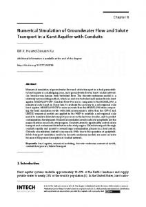
flooding through throat is shown in Figs. 5–7. The blue beads, red ones and purple ones represent water, oil and polymer, respectively. Since the value of α ˆ ij , repulsive parameters between bead i and bead j, control the miscibility of two fluids and the wettability of solid surface,13 the polymer is water-soluble (ˆ αPO > α ˆ PW ) and the purple beads are dispersed among the blue ones accordingly. Some fraction of oil adheres to the solid wall after flooding over the oil-wet throat surface (ˆ αWS > α ˆ OS ), but the oil is completely detached from the water-wet throat surface (ˆ αWS < α ˆ OS ). For an oil-wet throat, the surface tension between oil and water is opposite to the direction of external mass force, so the value of external mass force (the value is 0.025 in Figs. 5−6) must be large enough to overcome the surface tension, and make the fluid flow. On the other hand, the surface tension is in the same direction as the external mass force for a water-wet throat, so a very small external mass force (the value is 0.001 in Fig. 7) can make the fluid flow. It needs to mention that the contact angle is not fixed in the flooding process through the pore.

Fig. 7. Some snapshots of polymer flooding through a waterwet throat (F =0.001)

This work was supported by the National Basic Research Program of China (2005CB221307 & 2005CB221304), China Postdoctoral Science Foundation (20090460391 & 201003138) and PetroChina RIPED Innovations Foundation. Appendix rˆij = rij /rc , m ˆ = m/mDPD , vˆij = vij /U, ∆tˆ = ∆t × U /rc , Fˆi = Fi rc /U 2 × mDPD , α ˆ = αrc /U 2 × mDPD , γˆ = γrc /U × mDPD , √ ( )1 Pˆ e = mDPD U 2 /2kb T 2 = U/ 2UT , 1

Fig. 5. Some snapshots of polymer flooding through an oilwet throat (F = 0.025)

3 1 σ ˆ = σrc2 /(U 2 × mDPD ) = γˆ 2 /Pˆ e, n ˆ DPD = nDPD × rc3 , ˆb Tˆ = kb T /(mDPD × U 2 ) = 1/(2 × Pˆ e2 ), k ρ = (ˆ nDPD × mDPD )/rc3 , √ UT = kb T /mDPD , ˆ = (U × mDPD × n Re ˆ DPD )/µ × rc2 , ∆tˆ ≤ 0.1/ˆ γ, kb ≈ 1.381 × 10−23 (J/K) For water at temperature 330 K α ˆ = 75/(2 × n ˆ DPD × Pˆ e2 ),

ˆ ×n γˆ ≈ 1575/2π1/(Re ˆ DPD ),

Some preliminary studies on DPD simulations of pore-scale flows in chemical flooding process are presented in this paper. In our opinion, the numerical instabilities of many conventional methods can be avoided in this approach, and the simulation results can gain a clear physical insight into the flow of polymer flooding at the pore scale.

rc ≈ 3.104 × (ˆ nDPD × Nm )1/3 × 10−10 (m), mDPD ≈ 3 × Nm × 10−26 (kg), µ ≈ 0.523 (mPa · S). 1. S. P. Guo, Y. Z. Huang, and J. Zhou, et al., Porous flow with Physicochemical Process: Microscopic Mechanism, (Science Press, Beijing, 1990).

022008-5 Numerical simulation of pore-scale flow

2. A. John, C. Han, M. Delshad, and G. A. Pope, et al., SPE Journal, 10, 206 (2005). 3. K. Petros, Annu. Rev. Fluid Mech. 37, 457 (2005). 4. P. J. Hoogerbrugge, and J. M. V. A Koelman. Europhys. Lett. 19, 155 (1992). 5. R. Groot, P. Warren, and J. Chem. Phys. 107, 4423 (1997). 6. P. Espaˇ nol, and M. Revenga, Phys. Rev. E 67, 026705-1026705-12 (2003). 7. M. Amitesh, and M. Simon, J. Chem. Phys. 120, 1594 (2004). 8. E. Keaveny, I. Pivkin, and M. Maxey, et al, J. Chem. Phys.

Theor. Appl. Mech. Lett. 1, 022008 (2011)

123, 104107-1-104107-9 (2005). 9. C. A. Marsh, G. Backx, and M. H. Ernst, Europhys. Lett. 38, 411 (1997). 10. J. A. Backer, C. P. Lowe, and H. C. J. Hoefsloot, et al, J. Chem. Phys. 122, 154503-1-154503-6 (2005). 11. S. Chen, P. T. Nhan, and X. J. Fan, et al., J. Non-Newtonian Fluid Mech. 118, 65 (2004). 12. L. M. Wang, G. Wei, and J. H. Li. Computer Physics Communications 174, 386 (2006). 13. X. B. Li, Y. W. Liu, and J. F. Tang, et al., Acta Mech. Sin. 25, 583 (2009).