Severe short circuit was found through all outlets of a bare tundish. The flow ...... 3-D drawing of Volume of Tundish for simulation. 28. 3.2 a) Inner volume of the tundish with plane of symmetry after considering the refractory .... achieving straight exit after the appropriate combination of radius(R1= 9m, R2=16m and. R3=â).
NUMERICAL SIMULATION OF FLOW BEHAVIOR OF LIQUID STEEL IN AN 8 STRANDS TUNDISH OF CONTINUOUS CASTING MACHINE Submitted in partial fulfillment of the requirements of the degree for the degree of Master of Technology (steel technology) by Amiy Srivastava (Roll No. 133114012)
Under the supervision of Prof. N. N. Vishwanathan
Department of Metallurgical Engineering and Materials Science INDIAN INSTITUTE OF TECHNOLOGY, BOMBAY June, 2015
Abstract The flow behavior of liquid steel in an eight strand tundish was simulated using computational fluid dynamics software(Fluent-14.0). Bench-marking study was done to check the reliability of methods used in simulating the flow behavior. Grid independence study was also carried out to achieve the most precise solution. As a result, Residence time distribution (RTD) curves were drawn using Fluent post processing tools. Extensive analysis was done for a bare eight- strands Tundish first. RTD curves were correlated with velocity vectors and pathlines to visualize the flow closely. Flow behavior in a bare tundish was found highly unfavorable for cleanliness. Severe short circuit was found through all outlets of a bare tundish. The flow characteristic for all the outlets were found highly inhomogeneous. Flow modifiers were used in Tundish to alter the unfavorable flow of liquid steel in tundish. Flow behavior of liquid steel in all cases was studied and correlated it with vector plots and pathlines to predict exact flow behavior in different cases. Dispersed Plug volume fractions were calculated for different cases. Dispersed plug volumes in all cases were compared and found that in one arrangement when the combination of turbulence inhibitor, baffles and dams was used, the value of dispersed plug volume fraction was increased. A modified turbulence inhibitor was used in Tundish in one of the cases. The dispersed plug volume fraction for this case was also found high. Inhomogeneity and Short circuit flow were also reduced when these flow modifiers were used in tundish.
Table of Contents Chapter 1 Introduction ............................................................................................................................ 9 1.1Overview of Continuous Casting Process ...................................................................................... 9 1.2 Overview of Tundish .................................................................................................................. 10 1.2.1 Introduction to Tundish ........................................................................................................ 10 1.2.2 Requirement of Tundish....................................................................................................... 11 1.3 Design Criterion & Types of Tundish......................................................................................... 12 1.4 Different Tundish Issues ............................................................................................................. 14 Chapter-2 Literature Survey ................................................................................................................ 15 2.1 Brief description of use of some flow modifiers in Tundish...................................................... 15 2.2 Modeling of Flow behavior of Liquid Steel in Tundish ............................................................. 18 2.2.1Theory of Physical Modeling ................................................................................................ 18 2.2.2 Theory of Mathematical Modeling ...................................................................................... 24 2.3 Motivation for the research ........................................................................................................ 26 2.4. Objectives .................................................................................................................................. 27 Chapter 3: Model Development ............................................................................................................ 28 3.1 Drawing Construction ................................................................................................................. 28 3.1.1Construction of Isometric view on GAMBIT ....................................................................... 28 3.1.2 Meshing on GAMBIT Software .......................................................................................... 30 3.1.3 Defining Zone ...................................................................................................................... 31 3.1.4 Saving and Exporting the drawing ....................................................................................... 31 3.2 Procedures in Fluent 14.0 ........................................................................................................... 31 3.2.1 Material Properties ............................................................................................................... 32 3.2.2 Boundary Conditions ........................................................................................................... 32 3.3 Drawing RTD curves using Fluent ............................................................................................. 32 3.4 Conversion of F(t) into E(t) curve............................................................................................... 32 3.5 Method for Calculating Dimensionless Concentration and Dimensionless time ........................ 33 3.5.1 Converting E(t) to C(t) ......................................................................................................... 33 3.5.2 Converting C(t) to C(Ɵ) ....................................................................................................... 33 3.5.3 Converting t to Ɵ.................................................................................................................. 33 Chapter-4 Result and discussion ........................................................................................................... 34 4.1 Bench Marking............................................................................................................................ 34 4.2 Grid Independence Study ............................................................................................................ 36 Page | 1
4.2.1 Significance of the study ...................................................................................................... 36 4.2.2 Mathematical Work: Result through Plot ............................................................................ 36 4.2.3 Grid Independence Study by examining velocity vectors at some plane of interest ............ 37 4.3 Study of Flow Behavior of Liquid Steel an eight strands tundish .............................................. 40 All these cases are discussed in further sections of this report. Post-processing part of Fluent is used to define flow in all cases. The tools used to describe flow behavior are as follows:....................... 41 1.
RTD (Residence Time Distribution) curves ............................................................................. 41
2.
Velocity Vector plots at Planes of Interest and at 3-D space .................................................... 41
3.
Path-lines display ...................................................................................................................... 41
4.4 Case-0: Analysis of Flow Behavior of Liquid steel in a Bare Tundish....................................... 41 4.4.1 Analysis through Residence Time Distribution(RTD) Curves ............................................ 41 4.4.2 Flow analysis using vector orientation at different planes ................................................... 44 4.4.3 Description of Flow using Pathlines display ........................................................................ 51 4.4.4 Drawbacks of using a bare eight strands tundish ................................................................. 52 4.5 CASE-1: Low Height rectangular shaped impact pad with no back wall (H=84.324 mm) ........ 52 4.5.1 Residence Time distribution Curves for CASE-1 ................................................................ 53 4.5.2 Flow analysis using vector orientation at different planes ................................................... 55 4.5.3 Path-lines display for case-1 ................................................................................................ 56 4.5.4 Flow behavior explanation using some 3-Dimensional views ............................................. 57 4.5.5 Drawbacks of Tundish Model in CASE-1 ........................................................................... 58 4.6 CASE-2: Tundish with BOX TYPE Turbulence Inhibitor (H=160mm) .................................... 58 4.6.1 Description of Flow using RTD curves ............................................................................... 59 4.6.2 Description of Flow velocity vectors at some planes of interest.......................................... 61 4.6.3 Description of flow using Pathlines ..................................................................................... 63 4.6.4 Drawbacks of Case-2 ........................................................................................................... 64 4.7 Case-3: Tundish with Round Shaped Turbulence Inhibitor of More height (h=160mm) ........... 64 4.7.1 Description of RTD curves .................................................................................................. 65 4.7.2 Comparison study of vector plots at plane of symmetry ...................................................... 65 4.7.3 Description of Flow analyzing vectors plot at Horizontal Top surface ............................... 67 4.7.4 Flow Description using Pathlines Display ........................................................................... 67 4.7.5 Drawbacks of case-3 ............................................................................................................ 68 4.8 Case: 4 Round shaped modified Turbulence Inhibitor ............................................................... 68 4.8.1 Description of RTD curves in Case-4 .................................................................................. 69 4.8.2 Description of flow using vector plots at plane of symmetry .............................................. 72 Page | 2
4.8.3 Drawbacks of case-4 ............................................................................................................ 72 4.9 CASE-5: Small height round shaped Turbulence inhibitor & Dam (h= 360mm) ...................... 72 4.9.1 Description of flow using RTD curves ................................................................................ 73 4.9.2 Description of Flow using Pathlines .................................................................................... 73 4.9.3 Drawbacks of CASE-5 ......................................................................................................... 74 4.10 CASE-6: Box Type Turbulence inhibitor (h=160mm) and Dam (h=360mm).......................... 74 4.10.1 Description of flow using RTD curves .............................................................................. 74 4.10.2 Description of Flow using Pathlines .................................................................................. 75 4.10.3 Drawbacks of this Model ................................................................................................... 75 Fig 4.40. Baffle with rectangular slot a) Baffle-1 with 41oangle from horizontal, b) Baffle-2 with no angle from Horizontal, c) Baffle-3, slot slightly above the previous position in baffle-1 ................ 76 4.11 CASE-7 Round shaped Turbulence Inhibitor with slotted Baffle-1 ......................................... 77 4.11.1 Flow description using RTD curves................................................................................... 77 4.11.2 Flow Description using pathlines ....................................................................................... 78 4.11.3 Drawbacks of CASE-7 ....................................................................................................... 79 4.12 Case:8 Tundish with round shaped turbulence inhibitor, Baffle -2 and 2-dams ....................... 79 4.12.1 Description of Flow behavior using RTD curves .............................................................. 79 4.12.2 Drawbacks of Case-8 ......................................................................................................... 80 4.13 Case-9: Box-type Turbulence Inhibitor with slotted Baffle and 2 dams................................... 80 4.13.1 Description of Flow using RTD curves ............................................................................ 81 4.13.2 Description of flow using Pathlines ................................................................................... 81 4.13.3 Drawbacks of Case-9 ......................................................................................................... 82 4.14 Case-10 Tundish with Box type turbulence inhibitor, Baffle-3 and 2 dams ............................. 82 4.14.1 Description using RTD curves ........................................................................................... 83 4.14.2 Description of Flow using Pathlines display...................................................................... 83 4.14.3 Drawbacks of Case-10 ....................................................................................................... 84 Chapter-5 Conclusion & Suggestions for Future work ......................................................................... 85 5.1 Value of Plug flow Volume fractions ......................................................................................... 85 5.2 Homogeneity in Flow characteristic and number of peaks on RTD curves ................................ 85 5.3 Occurrence of Short circuit flow ................................................................................................. 86 5.4 Suggestion for the future work ................................................................................................... 86 6.0 APPENDIX ..................................................................................................................................... 87 7.0 References ....................................................................................................................................... 92
Page | 3
List of Figures: Fig No.
Details of figures
Pg. No.
1.1
Schematic representation of Continuous Casting Process with concerning area of Quality requirement
10
1.2
Schematic diagram of a tundish of 2 strands with arrangement described
10
1.3
Schematic Designs of different types of tundish
13
2.1
Schematic Diagram of Flow for 2-strands Tundish: Use of some flow modifiers
15
2.2
Alteration in Dead volume fractions because of using Flow Modifiers a) Dead Volume in a bear tundish is 24%, b) When Dam is used dead volume reduced to 17% and c) when weir is also used along with Dam, Dead Volume is increased to 27%
16
2.3
Different Configuration in a 6 strand tundish and corresponding RTD Curve for symmetrical 3 strands: a) Baffle with five holes configured six strands tundish, b) RTD Curves for strand 1, 2 and 3, c) Tundish configuration 1 or 2 with baffle 1 or 2, respectively d) RTD curves of tundish configuration with baffle-1
17
2.4
a)RTD curve for complete mixing,: b)Combination of Plug, dead and Mixed volume fraction, c)Typical RTD curves
21
2.5
RTD curves for six strands tundish
24
3.1
3-D drawing of Volume of Tundish for simulation
28
3.2
a) Inner volume of the tundish with plane of symmetry after considering the refractory thickness. b) final half geometry of a bare tundish(volume of interest for simulations)
29
3.3
a) Tundish Geometry with Separating Planes, b) Finer Mesh Propagating from Inlet mesh, c) Finer mesh at Inlet face, d) Coarser mesh at Inlet face
31
4.1
a) Tundish geometry in Cloete's Report, b) Developed for Benchmarking for current report: Plane of Interest: Plane-A (also a symmetry plane)
34
4.2
Velocity vectors on plane of symmetry-2 a). plane of Interest A in Quarter tundish made in current research b). Plane of symmetry in Cloete's Tundish
35
Page | 4
Model of a bare tundish
4.3
Velocity at inlet and each outlet for different number of cells
36
4.4
Schematic diagram of Bare Tundish and characteristic planes of Interest (Plane of symmetry and plane A)
37
4.5
Velocity Vector representation for Planes of Interest (a) Plane-A, (b) Plane of symmetry for (1) CASE-A(2) Case-B; (3) Case-C, (4) Case-D, (5) Case-E, (6) Case-F and (7) Case-G
38-40
4.6
RTD curves for bare tundish a) Outlet-1 (left side view), b) Outlet-2( left side view), c) Outlet-3 (full view), d) Outlet-4 (full view), e) Combined RTD Curves in Simultaneous View
43-44
4.7
Horizontal planes of Interest in a Bare Tundish
45
4.8
Vectors of fluid flow at the left side of the planes of the interest(near impact zone) and Rotation of Vectors shown using Red circle, Vector orientation through Black arrows (vertical axis, V and horizontal axis H are shown with dotted arrows).
46-47
4.9
Plane of Interest for Vector Investigation, Plane-1, 2 and 3(vertical planes)
48
4.10
a) plane-1 just above all outlets normal to y-axis, b)plane 2 just above outlet-2 normal to x-axis and recirculation zone(red circled).c) Vectors from right side intersecting the recirculation zone, d) Horizontal vectors directed towards outlet-3, Intersecting Vectors at Plane-3
49-50
4.11
Vectors between outlet-3 and outlet-4
51
4.12
Path-lines followed by Liquid steel at initial stages just after hitting the bottom surface of the tundish
51
4.13
Schematic diagram of Tundish for CASE-1
52
4.14
RTD curves for CASE-1: a) Outlet1, b) Outlet2, c) Outlet-3, d) Outlet-4, e) Combine RTD Curves in Simultaneous View
53-54
Page | 5
4.15
(a) Top layer of the Tundish of Case-1 (b) Black Circled shows Originpoint at top surface, Red arrows shows vector moving upward (3d view1)
56
4.16
Pathlines of fluid flow in case-1
57
4.17
View of the striking velocity vectors at the back wall of the tundish at sprouted region of tundish. (3- D view 2)
57
4.18
Contour of turbulence intensity: Black Circle shows effect on Back wall of tundish at sprouted region. (3d view-3)
58
4.19
Schematic Diagram of the tundish for CASE-2
58
4.20
a) Contour of Turbulent Intensity near tundish back wall at sprouted zone, b) Low magnitude velocity vectors (3-d View-1)
59
4.21
Combined RTD Curves in Simultaneous View for CASE-2(X-axis, Ɵ= 0 to Ɵ=2)
60
4.22
Plane of Interest where flow is analyzed
61
4.23
a) Formation of the recirculation zone at the left side of the plane just above the outlets, b) Planes parallel to the bottom plane showing straight direction of velocity vectors towards outlet 2, c) Recirculation zone shown within the black circle.
61-62
4.24
Set of Horizontal planes parallel to bottom plane and planes above outlets
63
4.25
Pathlines display of Flow (Recirculation zone extended vertically-Shown using orange circle)
63
4.26
Schematic diagram of Tundish of case-3
64
4.27
Combined RTD Curves for all outlets in a Simultaneous View
65
4.28
Velocity vectors at Plane of symmetry a) for CASE-3, b) for CASE-2
66
4.29
Top Plane of the tundish with round shaped more height Turbulence
67
Page | 6
Inhibitor 4.30
Pathlines display for case-3
68
4.31
Schematic diagram of the (a) Tundish for Case-4 and (b) Modified Turbulence inhibitor
68
4.32
RTD curves for case-4 a) Outlet1, b) Outlet2, c) Outlet-3, d) Outlet-4, e) Combine RTD Curves in Simultaneous View
69-71
4.33
Velocity vectors at Plane of symmetry for case-4
72
4.34
Schematic diagram of Tundish of CASE-5
72
4.35
Combined RTD Curves in Simultaneous View for CASE-5
73
4.36
Pathlines display for case-5 tundish
74
4.37
Schematic Diagram of tundish with Box-type Turbulence Inhibitor and Dam
74
4.38
Combine RTD Curves in Simultaneous View for CASE-6
75
4.39
Pathlines display for CASE-6
75
4.40
Baffle with rectangular slot a) Baffle-1 with 41oangle from horizontal, b) Baffle-2 with no angle from Horizontal, c) Baffle-3, slot slightly above the previous position in baffle-1
76
4.41
Schematic diagram of the CASE-7 tundish
77
4.42
Combined RTD Curves in a Simultaneous View for Case-7
78
4.43
Pathlines display for case-8(More pathlines are directed to outlet-2)
79
4.44
Schematic Diagram of the Tundish of Case-8
79
4.45
RTD diagram in a simultaneous view for Case-8
80
Page | 7
4.46
Schematic diagram of Tundish for CASE-9
80
4.47
RTD curves for CASE-9
81
4.48
Pathlines display for CASE-9
82
4.49
Schematic diagram of tundish for case-10
82
4.50
combined RTD Curves for Case-10
83
4.51
Pathlines display when length of pathlines is 150m
84
List of tables: Table No.
Details of table
Page No.
Table 3.1
Geometry of Internal Structure of Tundish
29
Table 3.2 Table 3.3
Physical Properties of Simulating fluid Initial and Boundary conditions
32 32
Table 4.1
Different cases with corresponding mesh interval size and number of cells
37
Table 4.2 Table 4.3
List of all cases studied in the current research Values of Volume fractions and tpeak, tmin and tmean for Case-0
41 42
Table 4.4 Table 4.5
Values of Volume fractions and tpeak, tmin and tmean for Case-1 Values of Volume fractions and tpeak, tmin and tmean for Case-2
55 60
Table 4.6
Values of Volume fractions and tpeak, tmin and tmean for Case-4
71
Page | 8
Chapter 1 Introduction Continuous casting had become very famous casting process in steel industries from last several decades to ensure high production along with no compromise with high end product quality. Continuous Casting machine consists of many arrangements made using engineering wisdom to aim at different problems encountered during casting through conventional method of ingot casting.
1.1Overview of Continuous Casting Process In the process of continuous casting, liquid steel is poured into the Tundish through a ladle shroud (made of refractory). Mass flow of steel is bifurcated into the number of strands. Liquid steel in the tundish is transported through opening between stopper rods and tundish well nozzle into the molds made of copper alloys having high values of heat transfer coefficient kept in a cartridge consists of cooling jacket for efficient heat extraction from steel solidifying shell at initial length of strand less than one meter(length of copper alloy mold). The opening of the stopper rods depends upon the level of liquid steel in the mould. The level is estimated by Mould level control (MLC) with the help of device which works on the principle of radioactive emission using Co60 (Cobalt 60, Isotope used in JSPL Angul, India's Caster of 8 strands). Aspiration of air is prone from the opening between stopper rod tip and tundish well nozzle due to negative pressure which becomes the reason of Alumina (Al2O3) clogging in the nozzle [1]. Steel poured in the mould, has been started getting solidified due to continuous heat extraction from the surface of mould. A rigid dummy bar arrangement is used for the pouring of first ladle of the sequence into the Tundish. Rigid dummy bar holds the liquid steel till it gets solidified up to some extent of shell thickness and then it gets ejected and disconnected achieving straight exit after the appropriate combination of radius(R1= 9m, R2=16m and R3=∞). The arrangement of withdrawal and straightener gives strands a straight shape and after this the Torch Cutting Machine starts its work to cut the billet/slab into required sizes. Billets are transferred to Turnover cooling bed for cooling to ambient temperature. Generally Magnetic cranes are used to lift the billet from TOCB (turn over cooling bed), if the temperature of billet is more than 770oC, magnetic property is lost and expensive cranes are used to lift the billet. Here, a complete overview of caster layout is given in figure.1.1 which describes the area of quality requirement and state of steel flowing in the caster. Our research in this thesis although deals with only one part of caster that is tundish therefore in the further sections onwards, overview of tundish will be given.
Page | 9
Fig.1.1 Schematic representation of Continuous Casting Process with concerning area of Quality requirement [2]
1.2 Overview of Tundish 1.2.1 Introduction to Tundish
Tundish is situated in a continuous casting machine beneath the ladle and above the copper mold, basically works as a buffer for casting continuously without interruption. When liquid steel is poured by one ladle, another ladle is kept on the other side of turret. Once the pouring ladle gets empty, the turret starts rotating half of the circle and moves down its one of the arms having new ladle towards the tundish. Slide gate attached at the bottom at eccentric position of the ladle bottom, is opened and ladle shroud is attached manually on the ladle opening with the help of a device works on the principle of first order lever. Tundish helps liquid steel to distribute into the strands and also provides some time to liquid steel element to stay in it and during this stay many metallurgical operations can be accomplished in terms of refining liquid flow and heat flow. Schematic diagram of a tundish is given in figure 1.2.
Fig.1.2. Schematic diagram of a tundish of 2 strands with arrangement described
Page | 10
1.2.2 Requirement of Tundish
Tundish facilitates in terms of quality improvement, higher productivity, slag free transfer, optimized metal delivery to the mold and effective thermal and chemical controls. Tundish plays an many important roles in continuous casting. Some are described below[3]. 1.2.2.1 Role as a Continuous Metallurgical Refiner
Liquid steel spends some time before being transported to the mould for casting; this time of stay is known as characteristic residence time In this time, inclusions may float-up with optimum fraction depending upon their diameter. Therefore modifying the flow behavior of the liquid steel in tundish may give rise to more and more inclusion floatation. Increasing the plug flow volume fraction increases more and more inclusion floatation. Three modes of inclusion removal is described i.e., flotation to the free surface, collision and coalescence of inclusions to result a change in size and shape and adhesion to the lining solid surfaces. Various phenomena occur during particle motion i.e. Brownian collision, Stokes collision, and turbulent collisions are studied by Zhang et al. [4]. They showed that not only through floatation but also through collision of inclusion and adhesion to the lining of solid surfaces, inclusion removal (for smaller size inclusions) can occur efficiently from molten steel in tundish. Tacke et al. [5] showed that inclusion rise to top slag layer achieving stokes velocity which is the consequence of density difference between molten steel and inclusions. Saeki et al. [6] defined tundish as a refining vessel with some following criterions: 1. Sources of molten steel contamination have to be eliminated. The main sources are refractory erosion, re-oxidation, ladle slag carryover and tundish slag emulsification. 2. Maximized Inclusion flotation and separation from the melt using flow modifiers filters and engineered slags. 3. Introduction of technologies such as thermal control, slag-free transfer and optimized metal delivery systems to the mold. 1.2.2.2. Role as a Transmitter of Metallurgical Signal
Tundish can also be used as a transmitter for metallurgical signals. Those signals are characterized as chemical signal, thermal signal, electrical signal, optical signal, vibrational signal and sonic and ultrasonic signal. Oxygen probes are used to check the proper working of gas shrouds (ladle to tundish transport) for minimizing the air aspiration. These monitoring methods can also be extended to control the rate of addition of the element such as aluminum or calcium and to monitor the effectiveness of their behavior on the basis of the estimated value of activity of the residual oxygen. The role of Nitrogen to find out the oxygen pick-up cannot be ignored. An increase in nitrogen content of 10ppm during transfer of liquid steel from ladle to tundish indicates that the oxygen pickup was around 2000 to 3000 ppm. This oxidation can lead to Alumina clogging in the shroud. [7] Thermal Signals can be obtained by mean of utilizing the technological advancement through continuous measurement probe (CMP) [8]. Difference between temperatures at some reference point positioned 240mm above the bottom of the tundish and the temperature at some points under consideration. A plot of this temperature difference Vs distance from the Page | 11
bottom of the tundish is shown by Maruki and Yamagata [8, 9] and found in the study that temperature difference is the function of the distance from the bottom of the tundish when the points under consideration are situated below 240mm. However above 240mm, temperature difference is independent of the distance from the bottom of the tundish. This is known as spot temperature measurement in the tundish. Continuous measurements and spot temperature measurement were compared with respect to time and found that continuous monitoring is better in the aspect of better quality. Nakajima et al. [10] showed that Electrical signals are obtained using an online method known as LiMCA (Liquid Metal cleanliness Analysis) to measure the non-metallic inclusions by means of number density and size distribution. Tundish level was also maintained with the help of electrical signals using the principle of electromagnetic techniques. Same are also used to detect the carryover slag from ladle to tundish [11]. Research was carried out in Sumitomo Metal Industries [12] to detect the slag entrained into the tundish using optical signals that is nothing but the difference between the emissivity value of slag and the liquid steel as well as difference between the diameter of stream having slag entrained and not having slag entrained into it. Vibrational signals were also found significant because of the fact that there is a difference in density between metal and the slag and due to this there was a change in momentum transfer to a refractory nozzle from molten steel when slag was entered into tundish by high velocity liquid metal stream. This change in momentum gives some vibrational movement to the nozzle as well as tundish. Itoh et al. showed [13] that if a continuous sensing of these vibrational signals is possible, the onset of carryover slag can be detected by monitoring liquid metal transfer continuously. Extent of volatile matter released into the molten steel for example calcium can be obtained through vibrational signals using an accelerometer [14]. Although this experiment of gas metal interaction was performed at laboratory furnace and significant arrangement was done for continuous monitoring. Ultrasonic signals from tundish were utilized to detect the slag inclusion and other reaction products in the liquid steel [15].It was found that reaction product formed after addition of calcium silicide into the liquid steel, could be detected preciously by the device based on pulse ultrasonic signal. The starting of vortex formation can be detected using ultrasonic techniques and efforts to construct a warning system were started [16].
1.3 Design Criterion & Types of Tundish Theory related to tundish design aspect has been evolved with the fact that issues related to steady state condition in which level of tundish remain constant and the issues related to unsteady and transient state condition which occurs during ladle change after the end of the casting sequence should be accommodated in the final tundish design. It has already been studied two decades ago that tundish design should not only take care for the fact that tundish acts as buffer between ladle and the mold. Hence while designing a tundish; important aspects have to be taken care to be called it an optimum design for proper chemistry and size of the casting products, capacity integration with steel melting shop, cleanliness requirement, necessity of flow modifiers, yield losses and use of devices for generating different signals for slag free transfer etc. Basic tundish designs (given in figure 1.3) refer different types of tundish such as Trough shaped (Boat type or bath tub shaped, B-type) tundish having a Page | 12
rectangular base and if the shape of the base changes it gives a different design under the same category of trough shaped tundish known as coffin-shaped and flared-trough shaped tundish. Trough shaped tundish is used for single or two strands slab caster. For casters having more number of strands cannot use such tundish because of the erosion of stopper rod due to turbulent liquid steel stream. To get rid of the problem of this erosion of stopper rod, a new design of tundish used having a sprout attached with the trough design i.e. T-shaped tundish, so that entry stream of liquid steel would hit the impact pad positioned on this sprout and would not erode the stopper rod, on the other hand this shape provides full metal head for delivery to all strand but leads to short circuiting. The V-shaped tundish provides larger ladle stream pour box and leads to more residence time for molten steel fluid elements. When the design of B-type and V-type is combined, C-type tundish design is evolved. There are some drawbacks of trapezoidal tundishes which are not having a rectangular base, in terms of higher refractory costs, tundish skull weights, size of tundish furniture and heat losses due to the greater amount of surface area exposure. A very special type of tundish design had been evolved in 1987 at Nippon Steel‗s Nagoya Works in Japan [17]. The H-type tundish removes the disadvantage of occurrence of unsteady state of dropping level in the tundish. This unsteady state condition also occurs during the filling of liquid steel in the tundish since level would not be constant. Two ladles pour liquid metal into tundish simultaneously to keep the level constant in H-shaped tundish. Even during the ladle change operation, level in main tundish where stopper rods are attached does not drop. This is an advantage in terms of quality equivalent in the IF grade steel (having very low carbon percentage less than 0.008%) casting during ladle change to the quality in the middle of the ladle under steady state condition. Due to large tundish level fluctuations heat losses through the tundish walls occurs with high rates and use of this type almost eliminates the fluctuations in tundish level hence this becomes another advantage of this type of tundish.
Fig1.3 Schematic Designs of different types of tundish [18] Apart from utilizing different tundish designs as discussed above, it was shown by Wolf [18] and Chakraborty [19] that depth of tundish also plays an important role in terms of inclusion floatation. According to their school of thought longer tundish with low operating depth are more efficient in the removal of inclusion. If the height of tundish is less for shallower tundish, reaching of inclusion particle to the slag layers will take less time due to less relative distance from melt to the slag interface. However there are some disadvantages of shallower tundish in terms of slag vortexing and reduced ability to dissipate the turbulent energy of liquid steel stream which cause excessive mixing and retention of large eddies. Therefore while finalizing the design of the tundish, a balance has to be taken care of. Therefore in view Page | 13
point of an optimum tundish design; it can be summarized that a tundish should have sufficient volume so that tundish level does not go down to occur vortexing and sequence breaking, an optimum tundish depth for efficient inclusion separation according to wolf and Chakraborty‗s school of thought, uniform flow distribution to all strands otherwise quality of billet or bloom would not be same, optimal residence time for optimum floatation of inclusion (removal of optimum size inclusion), a sluggish and inactive slag layer otherwise slag entrainment into molten steel has to be monitored and controlled by implication of devices based on signal achieved from tundish, thermal and chemical insulation otherwise there will be a detrimental effect on tundish shell made of steel and formation of sources for inclusion from bad quality refractory and use of proper tundish furniture to minimize dead volume and maximize plug volume fraction which leads to minimize tundish skull for achieving optimum yield.
1.4 Different Tundish Issues All design criterion in tundish take care certain tundish issues and these are discussed here for basic understanding. Inclusion Floatation is an issue to be dealt in tundish. Liquid steel fluid elements spend some time in the tundish known as residence time. For maximum inclusion floatation maximum plug volume fraction is required. The source of inclusion in tundish is the carry over slag from the ladle (micro droplets form), tundish slag, eroded particles of refractory wall, various chemical/steel deoxidation reactions etc. The size of the inclusion plays an important role in their floatation. Joo et al. and Ruckert et al.[20, 21] investigated that inclusions having high terminal velocity and larger diameter are more prone to be floated towards slag layer along with the placement of proper flow modifiers at appropriate position. Control on super heat is also an important issue to be dealt because if it is in higher side bulging of the strand may occur because of less thickness of shell formed due to slower solidification rate and desired microstructure will not be achieved and chances of grain coarsening will be more. Another very important issue is grade intermixing to be dealt in tundish. A tundish can bear several heats depending on the quality of the refractory used but it is not necessary that all the heats are of same grade therefore at some range of time tundish neither has previous grade and nor the newer one, there will be a mixing of the grade and overall grade cast during that period becomes downgraded. For minimizing this, the mixed volume fraction should be minimized. Generation of tundish skull is also detrimental to yield of a continuous caster however some amount of skull cannot be removed to save the cast from slag entrainment due to vortex formation, on the other hand, occurrence of dead volume may lead to chilling and there by the formation of skull can occur, therefore this issue has to be dealt significantly.
Page | 14
Chapter-2 Literature Survey 2.1 Brief description of use of some flow modifiers in Tundish There is various flow modifiers used in tundish which are also famous to be known as ―tundish furniture‖. Some are discussed here such as dams, weir, turbo pad, near strand dams etc. Dams increase the residence time so that tundish can be used as a refining vessel. Fluid stream will go directly to the mould without spending the significant time for proper inclusion removal. However, dam deviates the path of liquid stream to upward and then allows it to enter the mould strand. Such an activity increases the residence time for the fluid element for optimized inclusion removal. Dams are kept at A & A‗ positions in the fig.4. Weir as tundish furniture has also very important role since it restricts the steel stream to the regions where slag mixing due to stream turbulence occurs more than the regions where turbulent energy has been dissipated almost. The region of high turbulence interactions contains slag particles entrained in the molten steel and if the steel flow upward would not be restricted to these regions, it would become highly contaminated with entrained slag particles and with these slag particles steel would enter the mould. Weirs are shown at the positions W and W‗ in the figure.2.1. Heating the melt is another important task has to be done in tundish sometimes because temperature drop may occur for the first steel due to radiation therefore some near strand dams shown in figure 2.1, at position N and N‗, are used which accumulates molten steel and due to this heat of content of steel, temperature drop does not occur and premature freezing can be avoided.
Fig. 2.1 Schematic Diagram of Flow for 2-strands Tundish: Use of some flow modifiers Turbo-stop (Turbulence Inhibitor, TI, shown in figure 2.1) is also important furniture which bears the high turbulent energy of the liquid stream and makes an effort in term of the formation of a quiescent slag layer. Also prevention from short circuit flow can be achieved by hindering the quick flow of liquid steel from outlet near to the ladle shroud in a multistrand tundish. Turbulence in liquid steel stream gives rise to the rigorous mixing which increase the mixed flow volume fraction and decreases the plug flow volume fraction effectively. The design of various flow modifiers has become an area of interest for researchers in recent years. Several researchers have shown the influence of pouring region turbulence on flow behavior of steel in tundish. Morales et al [22] has shown that turbulence Page | 15
inhibitor effectively reduces the turbulent generated due to high Reynolds number stream of liquid steel. Advance pouring chamber inhibits the turbulence near the pouring region. Selection and position of turbulent inhibitors depends upon shroud position, submergence depth and design of tundish. Dead Volume fraction can be altered using flow modifiers [23]. a. b.
c.
Fig.2.2. Alteration in Dead volume fractions because of using Flow Modifiers a) Dead Volume in a bear tundish is 24%, b) When Dam is used dead volume reduced to 17% and c) when weir is also used along with Dam, Dead Volume is increased to 27% Anurag Tripathi from Tata steel, Jamshedpur [24] was motivated by the fact that flow modifiers are certainly very effective tools for modification of flow behavior but they reduce the effective volume of the tundish. In their recent research, it was shown that electromagnetic forces can also play an important role in terms of flow modification. 3-D MHD simulation was performed to study the effect of electromagnetic forces on flow behavior of liquid steel. Light was thrown on the fact that dependence on shroud location, submergence depth and design of tundish can be reduced if external forces are applied on the tundish. Innovative evolution of the use of electromagnetic forces can have the potential in terms of increasing effective volume. Electromagnetic force was incorporated as a volumetric source term in the momentum equation discussed previously. Validation of the model was done along with the analytical solution of Hartman problem. Hartman flow is a steady flow of an electrically conducting viscous fluid between parallel non conducting channels with an applied transverse magnetic field. The modification of source in the Navier stroke equation was used and rest equations are elaborated finely in his paper related to electromagnetic force and Lorentz force etc. An optimum value of magnetic field led improved value of plug volume fraction and effective inclusion floatation. For Multistrands Tundish when the number of strand is more than 3, great differences between RTDs, temperature and concentration distributions among strands were observed by researchers can affect the cast quality. Uniformity in Temperature and residence time for liquid steel elements till it reaches all outlets is mandatory for similar quality casting from all strands. Breakout and bulging occur due to short circuiting occurs for the fluid having less residence time because it would be hotter. On the other hand, when elements spend much higher residence time, the chances of occurrence of dead volume increases due to which Page | 16
clogging may occur due to large heat loss through the walls. Z. L. Cai et. al. [25], investigated flow behavior of liquid steel in two operating mode for six strands billet caster. One mode is known as ―Normal operating mode‖, when all six strands are in use and another mode is known as ―Abnormal Operating mode‖, when five strands out of six are in use for casting. Choosing the appropriate strand to be closed in case of abnormal casting, flow characteristics were measured in their paper. Investigating for the case of normal operating mode, tundish of six strands consists of baffle arranged in fashion shown in figure.2.3 below:
b.
c.
d.
Fig.2.3 Different Configuration in a 6 strand tundish and corresponding RTD Curve for symmetrical 3 strands: a) Baffle with five holes configured six strands tundish, b) RTD Curves for strand 1, 2 and 3, c) Tundish configuration 1 or 2 with baffle 1 or 2, respectively d) RTD curves of tundish configuration with baffle-1 In the figure 2.3a, the type of baffle shown restricts impact energy to less volume which is made up of six side wall. Impact of liquid steel having very high turbulent energy occurs from all six sides hence a kind of a conflux flow occurs which is unfavorable in terms of slag entrainment to the steel. The flow behavior observed using residence time distribution curve (figure 2.3b) also gives the idea of inhomogeniety in flow behavior which leads to quality variation from each strand. On the other hand, arrangement in figure 2.3c gives more volume to restrict the impact energy hence chances of slag entrainment become less which were more due to the formation of conflux flow in the former baffle arrangement. Numerically simulating the steel flow in tundish of 6 strands, Merder [26] found in the projection of velocity profile that fluid flow structure can be defined near the region which is Page | 17
bounded by turbulence inhibitor and the region which is not bounded by turbulence inhibitor. The region bounded by turbulence inhibitor, also known as near Gate region. This comprises more of the velocity vector having the direction upward towards the free surface. This circulation gives rise to accumulation of non-metallic inclusion into steel phase. The rigorous circulation may expose the metal by disturbing the slag layer over it. The formation of ―metal eye‖ increases the chance of reoxidation and leads to clogging of nozzle. Refractory of pouring region also gets eroded due high turbulent energy.
2.2 Modeling of Flow behavior of Liquid Steel in Tundish Two prominent approaches are physical and mathematical modeling for simulating flow in of liquid steel in the laboratory. 2.2.1Theory of Physical Modeling
An economic (compare to trials on real tundish) way of predicting phenomena occur in tundish related to fluid and heat flow of liquid steel. Physical model is constructed accounting geometrical, kinematic, dynamic and thermal similarities. Water is chosen because kinematic viscosity of water is similar to that of liquid steel. Along with this, water also provides a transparent medium in the tundish so that flow phenomena would be visible. Geometrical similarity is nothing but scaling of a real tundish into the tundish model. In this, the ratio of all lengths is maintained constant. Full scale model, having the ratio 1:1, elaborates actual control, however drawbacks are brought in terms of large water supply and large building spaces. In reduced scale water models, the value of ratio is less than 1, for 1:3 length ratio, ratio of area of faces should be 1:9 and ratio of volume of tundish should be 1:27. Ladle shroud, tundish well nozzle and insert pieces used in tundish are obviously designed with same scale. These reduced models are cost effective because of lower consumable quantity. The kinematic similarity is obtained for a tundish model when dynamic forces act upon the fluid element and profile of fluid streamlines are equivalent in terms of magnitude and direction. If system dynamics which are defined as some dimensionless number for example Froude, Weber and Reynolds number for the real tundish and model are equivalent, kinematic similarity can be achieved. Froude Number similarity, the ratio of inertial force to gravity forces is more significant in tundish flow than the similarity of Reynolds numbers, ratio of inertial force to viscous force and used in fluid flow through pipes or around object [27]. Froude number is basically used for drainage due to gravity. The experimental work of Singh and Koria [28] showed that the magnitude of turbulent Reynolds number under turbulent flow range in different tundishes was found equivalent, therefore Froude similarity is more important. The Froude number is given as follows: NFr = u2 / g.L, Where, u is fluid velocity and L is characteristic length of the water model. Choosing a proper geometrical scale factor, Froude similarity relations were calculated in terms of velocity and flow rate. The relations are as follows: Page | 18
Lm = x LP um = x0.5 uP Qm= x2.5 QP, Where x is the scaling factor [23]. Above relationship was obtained using length scale relationship and Froude number relationship. While designing the tundish well nozzle or metering nozzle, composite kinematic viscosity of liquid as well as gas (aspired due to negative pressure), inertia force and orifice friction factor as well as surface roughness have to be taken into account therefore Reynolds number similarity comes into the picture. Thermal similarity was ignored in initial water models but recent studies [29, 30] have shown that thermal phenomena shift the fluid flow behavior which is called inversion. Thermal phenomena occurs during the operation of ladle change since new heat mixes into the previous heat and shifts the flow and short circuiting of fluid element.etc to the strand may occur. Keeping the thermal phenomena into consideration, physical modeling has incorporated mixing of cold and hot water to simulate this unsteady state behavior. Many Techniques have been evolved because of continuous research carried out from last two decades. Water Modeling simulations are not only dependent upon the dye injection these days. Acid injection with pH tracking, saline solution injection with conductivity measurements and conventional or high-speed videotaping combined with tracer bead image resolution techniques have also come into the picture. Dye injection technique gives a plot of dimensionless concentration versus dimensional less time known to have very famous curve; the RTD curve which is abbreviated for Residence time distribution, gives an idea about fluid flow behavior in tundish. 2.2.1.1 Residence Time Distribution Curves (RTD)
P. V. Dankwerts in his study [31] showed the age distribution curves for the fluid elements staying and coming out of the reactor vessel on the basis of tracer pulse experiment. There are two types of RTD curves. One is the C-type and another one is F-type RTD. A pulse of tracer (KMnO4, etc.) is injected from the inlet of the tundish model made of Plexiglas, at time t= 0, and certain concentration of tracer is received at the outlet at time t>0. The concentration values of the tracer at the outlet is plotted with respect to time. When the tracer is injected as a pulse, the obtained curve is known as C-type RTD curve and when there is a continuous input of tracer into the Tundish from inlet, the curve obtained is called F-type curve. Conversion of concentration and time into dimensionless value is required so that the amount of tracer injected would not affect the curve characteristic. Concentration measured at outlet is divided by bulk concentration of tundish to convert it into a dimensional concentration. Bulk concentration is given by the following expression: [32] Cb = Mass of Injecting/ Volume of Tundish C* = C/ Cb, Where C is the concentration measured at the outlet of the Tundish Characteristic time, τ is defined as follows; τ = Volume of tundish/ overall flow rate of molten steel Page | 19
The dimensionless Time corresponds to the C* is ϴ, which is described as follows: ϴ = t/ τ, where t is the time corresponding to C obtained at outlet. A distribution curve is found due to the fact that all the fluid elements spend different time in a reactor vessel. The overall flow volume of fluid elements in vessel say Tundish consists of plug flow volume, mixed flow volume and dead flow volume. Plug flow volume fraction is the most desirable volume fraction in term of inclusion floatation and mixed flow fraction as well as dead volume fraction has to be minimized. Total volume, plug volume, mixed volume and dead volume are denoted by vt, vp, vm and vd respectively. vt = vp + vm + vd (1) Plug volume fraction, Vp = vp / vt = vp / (vp + vm + vd ) similarly, ...............(2) Mixed volume fraction, Vm = vm / vt = vm / (vp + vm + vd) ..........................(3) Dead volume fraction, Vd = vd / vt = vd / (vp + vm + vd) ...............................(4) Using equation (1), (2), (3) and (4), equation of fraction can be obtained, Vp + Vm + Vd = 1 ..........................................................................................(5) In Plug flow Volume, also called ―Piston Flow, elements do not forerun each other. The fluid elements enter the vessel in a moment with constant velocities and parallel paths also leave the vessel with same velocities and parallel paths. Plug flow volume is the region between the well mixed volumes and strands. Since perfect piston flow is impractical due to some longitudinal mixing occurred by viscous effect and molecular or eddy diffusion. Minimum Residence time (ϴmin, Dimensionless) is the ratio of time taken by the first element of the tracer to reach the outlet nozzle to characteristic time. Peak residence time (ϴpeak, Dimensionless) is known to be the time when dimensionless concentration was found maximum. Average residence time is given as follows: tAvg =
∞ C 0
∗ tdt/
∞ c 0
∗ dt
All types of volume fractions such as plug volume, dead volume and mixed volume can be related to dimensionless time, ϴ. Vd = 1- ϴAvg ......................(6) VP = ϴpeak = ϴmin.................... (7) Vm = 1/Cmax ......................(8) For equation (6), it can be said that ϴAvg is the total dimensionless average time till the cutoff point equals ϴ=2. This value will be less than unity and if deducted by 1, it gives the dead volume fraction. It can be interpreted by equation (7), that if much amount of tracer reaches any strand due to short circuiting, the time taken to achieve the maximum concentration Page | 20
becomes short and plug volume fraction decreases. Similarly a quick flow of tracer into any strand shows shortening of minimum residence time hence plug volume fraction decreases. For equation (8), it can be described that if an increase in maximum concentration is detected, it means that mixing of tracer into the tundish bulk was less and mixed volume would be decreased then. Minimum dimensionless time when concentration of the tracer is detected at the outlet nozzle is maximum is equal to the plug volume fraction. The advent of fluid element at ϴmin also predicts that tracer concentration is highest; this is the reason why this time is also called ϴpeak. However such model was discarded at the initial stages of studying flow in tundish because some researchers had come-up with the fact that there must be some longitudinal mixing, hence plug volume defined in the previous model will be altered. Y.Sahai [23] had showed in his paper that a kind of scattering was found in the duration between the time at which maximum tracer concentration and the minimum break through time was occurred in experimental RTD curve in means that increase in tracer concentration was not sudden which shows that ϴpeak ≠ ϴmin in pragmatic situation and the addition of plug, mixed and dead volume fraction is also not equal to unity in real experimental situations. This scattering in plug flow is famous as dispersed plug flow in the modified form of ―Mixed Model. In this proposed model total volume of tundish is divided into dispersed plug volume, mixed volume and overall dead volume. Accommodating the effects of longitudinal mixing, the sum of all volume fractions came up to unity.
Fig.2.4 a)RTD curve for complete mixing,: b)Combination of Plug, dead and Mixed volume fraction, c)Typical RTD curves The RTD curves are the combination of dispersed plug flow, mixed volume flow and dead volume flow. Figure 2.4a is the RTD curve which has only mixed volume. In figure 2.4b, a Page | 21
combined model is shown. the result of addition of all such flow is a typical RTD curve which is shown in figure 2.4c. The modified equations are as follows: Vd = 1- ϴAvg Vdp = (ϴmin + ϴpeak)/2.......................9 Vm = 1- Vd - Vdp...............................10 Y. Sahai and T. Emi [33] described ―Dead Volume by dividing it into two types; fluid is fully stagnant in the region of first type and the fluid is not even able to enter this region. Since the characteristic time for a given tundish will remain constant at constant flow rate, there must be some faster moving fluid in the tundish equivalent to the dead volume to make the characteristic residence time constant. This faster moving fluid does not stay in the tundish for the sufficient time which is mandatory for Inclusion removal. On the other, slower moving dead region fluid loose sufficient heat and may lead to solidify. The fluid in this region moves very slowly therefore fluid stays for much longer time in the region and exchange of fluid between dead region and active region (defined as the combination of plug flow and well mixed flow), occurs continuously. The fluid which stays for the time longer than two times the mean residence time is defined as Dead Volume. Further regarding dead volume, it was defined that the fluid which stays for longer residence time, an equivalent amount of other fluid which is not in this region posses shorter residence time. However dead region in the tundish is not completely stagnant although its slowly moving hence a correction factor has to be introduced to find out the values closer to the reality. Inculcating the correction factor following formula can be used to estimate the dead volume: Vdv= 1-(Qa/Q)* ϴAvg ......................11 where Qa/Q = Area under the curve of dimensionless Concentration Vs dimensionless time from ϴ=0 to ϴ=2 and fractional volumetric flow rate through the active region. this value is always be less then unity and has to be taken care while calculating the fraction of dead volume. Here ϴAvg is calculated from ϴ=0 to ϴ=2. 2.2.1.2 Concept of Sub-Tundish for Multi-strands Tundish
In case of a multi strand tundish, sub-tundish concept was used by many researchers [25] to define the flow structure using RTD curves. for an n-strands tundish, it was supposed that there are n-sub-tundishes . The volume of liquid steel in ith sub-tundish correspond to ith strand is Vi , which can be given using following equation: Vi = (qi/
n i=1 qi)V...........................
12
qi= Volumetric flow rate of strand i V= Volume of liquid steel in tundish, m3 If volumetric flow rates for all the outlets is identical, V=nVi , Page | 22
the amount of tracer flowing out from the outlet i in time dt can be expressed as follows: dwi =Ci(t)qidt, total amount of tracer flowing out from the ith outlet is: wi =
∞ Ci 0
t qidt
The residence time distribution density function: ∞ (Ci 0
t qi/mi)dt =
∞ E 0
t dt = 1.............................13
The characteristic time or theoretical mean residence times for ith strand sub-tundish and nstrands tundish will be equal because total flow rate from all outlets will be the addition of individual flow rates and total volume of tundish will be equal to the addition of all volumes of sub-tundishes. tch,i = Vi/qi = V/
n i
qi = tch
Now for the sub-tundish i , the dead volume fraction is as follows: Vdv,i = 1-(Qa,i/Qi)* ϴAvg where, Qa,i/Qi = Area under the curve of dimensionless Concentration Vs dimensionless time from ϴ=0 to ϴ=2 and fractional volumetric flow rate through the active region for the i th sub tundish. Similarly dispersed plug volume fraction can be calculated for ith sub-tundish: Vdp,i = (ϴmin,i + ϴpeak,i)/2 ϴmin,i and ϴpeak,i can be calculated using RTD curve for the ith sub-tundish. Mixed Volume fraction can be given by as follows: Vmv,i =1-Vd,i-Vdp,i The total average volume fraction can also be calculated for whole tundish using the values of volume fractions for individual outlets. general equations for calculation are given as follows Vdpv= (Vdpv,1 + Vdpv,2 + Vdpv,3 + ..................+Vdpv,n)/n
and .................. 14
Vdv= (Vdv,1 + Vdpv,2 + Vdv,3 + ..................+Vdv,n)/n ,. ................................15 here n is the number of outlets; Vmv,i =1-Vd,i-Vdp,i The peaks of RTD curves also predicts the nature of fluid flow in the tundish. It depends upon the non-dimensional width of a tundish which can be obtained by ratio of width to Page | 23
length (w/L). For the tundishes having more w/L ratio, there RTD curves show two peaks. Residence time distribution curves were also drawn by T. Merder [26] for a six-strand tundish shown in the figure 2.5. It can be clearly seen that short circuit flow occurred at the outlet which is situated nearest to the inlet shroud. Since, a Box-type turbulence inhibitor was also used in their Tundish, the peak concentration time for outlet-2 was decreased compare to the outlet-1. It is probably because of the box type turbulence inhibitor which directs the liquid steel stream upward and directed to outlet-1. On the other hand, the shape of their tundish is delta not the T-shaped.
Fig.2.5 RTD curves for six strands tundish [26] 2.2.1.3: General Observations from Residence time distribution Curves
RTD curves shown in this research have C(Ɵ) in vertical axis and Ɵ in horizontal axis. From the behavior of RTD curves many observations can be drawn. For example If the peak of dimensionless curve attained at much higher dimensionless concentration at very less dimensionless time in any RTD curve for any outlet, it is short circuit flow occurred at particular outlet. If the spread of RTD curve is more the dead volume fractions will be less for the particular outlet. More than one peaks in RTD show that some dead volume is releasing in time lags. Homogeneity in RTD curves for all outlets can also be observed seeing all the curves in a simultaneous view. If all curves for all outlets are of almost same structure the homogeneity will be more otherwise it is less. In case of less homogeneity, the thermal property of fluid flowing through all outlets may be different. Some calculated results using RTD curves may also predict the flow behavior. For example, if mean residence time is less than the theoretical residence time for any outlet, it is also one of the indications of occurrence short circuit flow at particular outlet. If peak dimensionless concentration is higher, more amount of fluid is flowing through that outlet. 2.2.2 Theory of Mathematical Modeling
Mathematical Modeling has become very famous tool to simulate various flow phenomena in tundish numerically. All types of flow behavior can be modeled using the principle of conversion of physical quantities such as viscous Momentum, advective momentum, force due to pressure and gravity. Mathematical Modeling has become very important because it saves hit and trial wastages and expenditure in terms of time and money in experiments. It Page | 24
also works as link between a water model and real tundish, once solution from mathematical model are validated with the physical model, those can be applied to the real tundish. Number of variations can be achieved in Numerical Simulation such as changing the configuration of tundish is possible in less time with no use of consumables. Many softwares have been evolved with the capability to define fluid flow behavior using appropriate boundary conditions, these softwares are known as CFD (Computational Fluid Dynamics) softwares and available with continuous increasing computational power in updated versions. Ansys Fluent along with GAMBIT (used for mesh designing) is also very useful software in term of better user- interface. Open Foam is also known to be very famous among students due to its free availability and easy accessibility. Flow behavior of a fluid element can be estimated when its velocity in x, y and z direction and pressure exerted on the considered fluid element are known. Such variables can be estimated using famous Navier Stokes Equation along with equation of continuity. Flow in tundish is highly turbulent and modeling of the turbulent stream needs a lot of computational cost but it is essential too. Therefore to reduce the computational cost, well known turbulence
ĸ-ԑ
model was used by several researchers [34]. The description of this model is given in APPENDIX of this report. Another equation used by CFD software is the famous equation of continuity and along with that appropriate boundary conditions for wall and free surface are required to simulate flow behavior in less computational time. Several researchers have found mathematical modeling a very useful tool to find out analytical RTD curves also using tracer dispersion equation along with previous equations and boundary condition. Numerically simulated RTD curves are compared with physically modeled RTD curves to check the validity of Mathematical observations. 2.2.2.1 Governing Equations in Mathematical Modeling
Although detail of governing equation is given on APPENDIX, let's see the glimpse of equations here also: The General Navier Stokes Equation is as follows: (∂ui/∂t) + ∂ (uiuk)/∂xk = (-1/ρ) {∂P/∂xi} + ν∇2ui Where i, j and are x, y and z-direction in Cartesian co-ordinate system. The expansion of this equation is given in APPENDIX. The equation of continuity: For incompressible flow, (∂u/∂x) + (∂v/∂y) + (∂w/∂z) = 0 along with this the equation of a turbulence model has to be used for capturing turbulence with the available computational power. 2.2.2.2 Boundary Conditions
While assigning the boundary condition into the CFD solver, extreme care has to be taken care otherwise a huge variation may occur in the final result. This variation may be yielded when initial condition assigned to fluctuating components is erroneous. Appropriate Page | 25
boundary conditions for inlet region, exit region, free surface and solid wall have to be given. Launder and Spalding [34] thoroughly documented that momentum defined by velocity components in x, y and z direction along with scalar quantities such as turbulent kinetic energy and its dissipation for turbulence ĸ-ԑ model, were modeled using wall functions since flow properties near the solid wall, changes drastically if are compared to in the bulk of liquid steel. At the solid walls, no slip boundary conditions were imposed. [35, 25] u=0, v=0; Free surface is considered quiescent say flat surface. Numerical interpretation is given in K.C. Hsu and C.L. Chou‗s paper [35] for free surface boundary: (∂u/ ∂y) = 0, v=0; At the jet entry, the velocity is normal to the free surface, (v= 4Q/пd2), flat velocity profile was assumed [35]. u= 0, v= constant; For exit same boundary conditions are applied, u= 0, v= constant; Plane of symmetry is defined as mirror plane from where if the tundish is cut; it will be divided into two identical parts, u=0, (∂v/∂x) = 0; 2.2.2.3 Tools to achieve results in Mathematical Modeling
There are so many post-processing tools available to obtain the results in CFD(Computational Fluid Dynamics) and out of them some are listed following: 1. 2. 3. 4. 5.
Velocity vectors orientation and their magnitudes at different planes of Tundish Turbulent kinetic energy and Turbulent Intensity Contours of Variables Path-lines RTD(Residence time Distribution curve of both F-type and C-type)
2.3 Motivation for the research JSPL, Angul, India has an eight strand billet caster which casts 165mmX 165mm billets. The Tundish used in this caster is an eight strand tundish. A bare tundish was used for casting billets of 165mmX 165mm and no flow modifiers were used to cast some grades. Square billets were casted by the policy of eliminating the sources of inclusions hence proper spray mass was applied as a refractory which did not get eroded. A proper flow structure of liquid steel is required to have maximum inclusion removal and to save from break-out occurred due to thin shell thickness. Selection of appropriate flow modifiers has become a tedious job. It has already been seen that an improper placement of flow modifiers can alter the flow characteristic significantly to an undesirable flow behavior. On the other hand, since the Page | 26
tundish has more number of strands therefore occurrence of short circuit may lead to detrimental effects on quality because same quality was required for all cast billet from all strands. Therefore optimum flow behavior has to be achieved to overcome various tundish issues. Chances of Formation of chilling zones at farther outlets are also there since the length of tundish is so long( Approximately 4.5 m from inlet shroud) On the other hand, slag line erosion was also a big issue at the impact zone. Therefore, this research is motivated by the above mentioned problems related to Tundish.
2.4. Objectives a). To simulate flow behavior of liquid steel in a bare Tundish and finding the problems with bare tundish. b). To simulate flow behavior of liquid steel in Tundish with flow modifiers to minimize the following issues: Minimizing Short circuit flow Maximizing Plug volume fractions Achieving Homogenization in flow characteristic of liquid steel flowing through all outlets of the tundish.
Page | 27
Chapter 3: Model Development The Tundish Model was made using GAMBIT(Geometry And Mesh Building Intelligent Tool) provided by Simmetrix Inc., 2002 and Ansys Fluent-14.0(Educational Version). The steps of model Developments are as follows: 1. Constructing Geometry 2. Creating Mesh on Constructed Geometry 3. Importing Meshed Geometry on CFD platform software 4. Running calculation and saving solutions 5. Post Processing: Finding RTD and Velocity Vectors
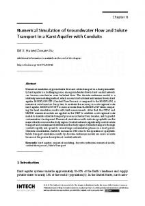
3.1 Drawing Construction The steps of drawing construction are as follows: 3.1.1Construction of Isometric view on GAMBIT The geometry of tundish was made using the dimension given in table 2.1. In figure 3.2, the dimensions are labeled and values of dimensions are given in table 3.1. The drawing shown was taken after considering bath level and refractory thicknesses.
Fig3.1 3-D drawing of Volume of Tundish for simulation
Page | 28
Table 3.1 Geometry of Internal Structure of Tundish Name of the length A B C D E F G H I K L M ARC LENGTH WHERE TWO VERTICAL SURFACES ARE COINCIDENT
Measurements in Meter 1.02 0.96 0.98 0.96 0.99 3.46 0.99 0.39 8.92 0.99 9.06 1.08 0.41 0.26 1.2 0.250 0.050 0.019
RADIUS OF ARC DISTANCE BETWEEN CENTERS OF THE OUTLETS SHROUD BELOW SLAG LAYER DIAMETER OF INLET DIAMETERS OF OUTLET
Only half of the tundish could be simulated to save computational time since one symmetrical plane can be found in the tundish which works as a mirror plane for the half of the whole volume of the tundish. The number of grid elements had been reduced for half tundish. The symmetrical plane can be seen in figure.3.2a. The half tundish bare tundish is shown in figure 3.2b. Plane of symmetry
Inlet
Outlet1
Outlet2
Outlet3
Outlet4 Outlet1
Page | 29
Outlet1'
Outlet2'
Outlet3'
Outlet4'
Fig 3.2 a) Inner volume of the tundish with plane of symmetry after considering the refractory thickness. b) final half geometry of a bare tundish(volume of interest for simulations) 3.1.2 Meshing on GAMBIT Software Instead of selecting complete half volume of tundish for creating mesh, small volumes were created by dividing the whole tundish. All those volumes were connected by separating planes shown in Fig. 2.4a. The boundary condition for such planes connecting small volumes was assigned as ―Interior‖ on GAMBIT. Finer mesh was created in Inlets and outlets and coarse mesh was created in volumes. Mesh propagates from Inlet face to the rest of the volume shown in Figure 3.3(b). Finer mesh is created because the inlet and outlet faces are circular and choosing maximum number of mesh element makes calculated mass flow rate equal to the mass flow rate of fluid flowing through inlet and outlets calculated by Fluent. If number of Mesh element is less at the inlet and outlet faces, the area covered by the mesh elements would be less than theoretically calculated area of the circular inlet and outlet faces which leads to the reason behind difference in theoretical mass flow rate and calculated Mass flow rate by Fluent software. The difference in covered area by mesh on circular inlet can clearly be seen in Figure. 3.3(c) and (d). Near the periphery of the circular faces, mesh is not able to cover the circular area which reduces the value of calculated area at inlet by Fluent software. Same problem occurs in case of Outlets if mesh is coarser. The Number of Mesh elements was chosen based on Grid Independence study discussed in next chapter. SEPARATING PLANES
Page | 30
Fig 3.3 a) Tundish Geometry with Separating Planes, b) Finer Mesh Propagating from Inlet mesh, c) Finer mesh at Inlet face, d) Coarser mesh at Inlet face 3.1.3 Defining Zone
On GAMBIT, zone has to be defined for particular material. In the present case, all volumes of tundish will contain only liquid steel (for steady state simulations) hence only same zone of liquid steel can be chosen for all small volumes on GAMBIT. 3.1.4 Saving and Exporting the drawing
Gambit drawing was saved in ".dbs" format and exported into ―.msh‖ (mesh file) format so that it can be imported to Fluent software for further procedure.
3.2 Procedures in Fluent 14.0 Fluent 14.0 solves the governing equations with appropriate turbulence model to capture the fluid flow in a closed container. The appropriate parameters like density, viscosity of the material have to be defined on Fluent software as input which should be realistically identical to the plant running conditions. Appropriate boundary conditions also have to be assigned for close solution. As a solution, vectors, contour, path-lines display can be achieved. Along with these results, Mass flow rate at each outlet and inlet can be calculated on Fluent-14. The assumptions for the current study are as follows: 1. The flow is dynamically steady means height of the bath is independent of time and it is constant.
Page | 31
2. All the calculations will be carried out in Cartesian co-ordinate system. 3. Flow in Tundish is highly Turbulent. 4.Tundish is kept at isothermal condition hence temperature variation was not taken into consideration, only flow properties were considered. 3.2.1 Material Properties
Liquid steel was chosen as a simulating material in the model. The properties of liquid steel are listed below in table 3.2. Table 3.2 Physical Properties of Simulating fluid Properties Density(kg/m3) Viscosity (kg/m.s)
Liquid Steel Model 7500 0.0064
3.2.2 Boundary Conditions
Initial and Boundary conditions used in simulation are shown in table 3.3. Table 3.3 Initial and Boundary conditions Boundary Condition at Fluent Inlet Hydraulic Diameter (inlet) Turbulent Intensity for Inlet Outlets (1-4) Turbulent Intensity for Outlet Hydraulic Diameter (Outlet) Top layer of Tundish
Details Velocity Inlet, 4.7 m/s 0.050m 5% Pressure Outlets 5% 0.019m Shear stresses Ʈxy=0, Ʈyz=0, Ʈzx=0, Full slip Condition
3.3 Drawing RTD curves using Fluent Similar to the Physical modeling, Residence time distribution curves can also be found using Fluent-14 software. Drawing RTD curves using fluent software is the part of post processing and on Fluent-14, both F-type and C-type of curve could be obtained. C-type RTD curves can be obtained using a pulse injection in which a virtual tracer pulse is injected from Inlet face for 5 seconds only. For F-type curves, continuous tracer is injected from the inlet face. However, both the curves can be converted into each other. The method of converting F(t) into E(t) is given in further section. The value of diffusion co-efficient for the tracer material has to be kept zero so that it does not react with the fluid in the tundish volume.
3.4 Conversion of F(t) into E(t) curve E(t)= d{F(t)/dt} Differentiation of F-type RTD data gives E-type RTD data and E-type RTD data can be used to get E-type RTD curves. In further sections conversion of E(t) into C(t) is explained.
Page | 32
3.5 Method for Calculating Dimensionless Concentration and Dimensionless time 3.5.1 Converting E(t) to C(t)
C(t)= E(t)*(user scalar Boundary Value)/ (Volumetric flow rate from one outlet) 3.5.2 Converting C(t) to C(Ɵ)
C(Ɵ)= C(t)*Volume of Tundish/ (4* user scalar Boundary Value) here, 4 was multiplied to user scalar Boundary Value to find total tracer amount injected from inlet 3.5.3 Converting t to Ɵ
Ɵ= t/Ʈ, where Ʈ is characteristic time spends to fill or empty the tundish. Using the formulae given in section 3.4.1, 3.4.2 and 3.4.3, the dimensionless C-curves can be obtained. The Model Developed should assure the followings for achieving the correct and reliable solution: 1. Solution should be grid Independent. 2. Solution and calculation methods should be benchmarked and validated with other models for checking the reliability of current numerical solutions.
Page | 33
Chapter-4 Result and discussion 4.1 Bench Marking Benchmarking is required to check whether our results match with real and practical situations or not. To check the preciseness of our numerical simulation, it was mandatory to benchmark some validated research work with the same method used in the current research. For this Cloete's Master's Thesis has been chosen. The Tundish geometry given in the work of Kumar et.al[37] with 1:2 scale was chosen in Cloete's Master's thesis. Fig.4.1a shows the geometry chosen by Cloete in his thesis.
A
Inlet Outlet-2
Outlet-1
Fig.4.1 a) Tundish geometry in Cloete's Report, b) Developed for Benchmarking for current report: Plane of Interest: Plane-A (also a symmetry plane) The diameter of Inlet shroud in Cloete's Tundish model was 30 mm and Outlets diameter was 10.5 mm. The velocity of liquid steel from inlet was 0.605 m/s and turbulence intensity was 5%. A quarter tundish was made since 2 symmetry planes could be found. Number of cells were 165639 in a quarter tundish made in the current study to benchmark Cloete's Tundish Model. The quarter tundish made in the current research work is shown in Figure 4.1b. The planes of interest, A was chosen to examine the velocity vectors in the current study. The vector plots at the plane of interest, A are shown in figure 4.2a and the vectors plot given in Cloete's thesis is shown in figure 4.2b. The direction of velocity vectors at plane of interest, A is found to be similar to the velocity vectors lying on the plane of symmetry in Cloete's thesis. The maximum range of Velocity magnitude is same in current study with Cloete's Models for same plane i.e. 0.002m/sec. The colors of vectors correspond to the magnitude of velocity at both the plane. The magnitude of velocity vectors can be drawn using the range color chart shown adjacent to the vectors plots in both the figures. It is found that magnitudes of vectors are also same in both the plots. Since positions, orientations and magnitudes all are same at both the planes, the method used in current research is also appropriate and benchmarked correctly.
Page | 34
Fig 4.2. Velocity vectors on plane of symmetry-2 a). plane of Interest A in Quarter tundish made in current research b). Plane of symmetry in Cloete's Tundish Model of a bare tundish
Page | 35
4.2 Grid Independence Study 4.2.1 Significance of the study
Method to achieve numerically simulated results through CFD (Computational fluid dynamics) is different from the method to achieve analytical solution of any equations. A solution can be found using both the method. However Analytical methods have limits when they deal with complex and large domain. Analytical solutions give exact solution to the equation within the temporal and spatial domain but Computational Fluid Dynamics(CFD) gives solution at discrete points. These discrete points are known as grid points. More the number of elements or cells, more will be the grid points. If discrete points are close to each other the solution will be precise for the particular flow domain. Therefore, more number of grid points assures closeness to the real solution. 4.2.2 Mathematical Work: Result through Plot
In the Grid independence study, the sensitivity of solution is examined with respect to number of grid points( or number of cells). For Grid Independence study in the current research, total 33 Models consist of different number of cells are made in same geometry of a bare tundish. The magnitudes of Velocity(considered as solution) are monitored at the centre of the all outlets . The plot of variation in velocity magnitudes at the centre of all the outlets with number of cells is made.
V E L O C I T Y
NUMBER OF CELLS
Fig4.3 Velocity at inlet and each outlet for different number of cells The plot obtained is shown in Figure.4.3. It is observed from the plot that when the number of cells were less(in the range of thousands), the magnitude of velocity were changing significantly and as the number of cells(or grid points) increases, the change in magnitude of velocity for individual outlets, is not significant. Further increasing the number of Page | 36
cells(thereby increasing grid points), a flat region is found in the plot (circled with a black color). This region is called a flat region of the plot because magnitude of velocity is not changing with further increase in the number of cells. 4.2.3 Grid Independence Study by examining velocity vectors at some plane of interest
The orientation of velocity vectors are examined at some planes of interest for the same bare tundish. The schematic diagram of bare tundish with plane of interest to examine the velocity vectors is shown in figure 4.4. Plane A
Plane of Symmetry
Fig.4.4 Schematic diagram of Bare Tundish and characteristic planes of Interest (Plane of symmetry and plane A) Some models are chosen from total models made for grid independency to examine the velocity vectors at planes of interest. Each selected model is specified as a case in the study given below. For each Case, the velocity vectors plots at plane of interest A and Plane of symmetry, are made. These vector plots are shown in figure 4.5. Selected cases are listed with their corresponding number of cells and Interval size between grid-points in the table 4.1. Interval size is defines as the spacing between grid points. If it is less, number of cells will be more. Cases are named as case A to case G. Table 4.1 Different cases with corresponding mesh interval size and number of cells CASES A B C D E F G
Page | 37
Interval Size 0.095 0.05 0.04 0.024 0.021 0.02 0.018
No. of Cells 4948 38913 78025 753510 881274 939270 1073676
1.
b.
a.
2.
a.
b.
a.
b.
3.
Page | 38
4.
a.
b.
5.
a.
b.
6.
a.
Page | 39
b.
7.
a.
b.
Fig.4.5 Velocity Vector representation for Planes of Interest (a) Plane-A, (b) Plane of symmetry for (1) CASE-A(2) Case-B; (3) Case-C, (4) Case-D, (5) Case-E, (6) Case-F and (7) Case-G It can be observed from figure 4.5 that the velocity vectors at the planes of interest for case A, B, C are changing significantly but moving further to the latter cases D, E F and G, it can be found by minute observation that orientation of velocity vectors are not changing and the flow is completely developed. The recirculation zones have been developed and their positions are also the same in latter cases. It can be concluded here that a further decrease in number of cells will not change the orientation of vectors and position of recirculation zones as these are not changed from case-D to G. Above evidences, the examination through variation plots and vector plot, are enough to prove that now the solution has become grid independent. A grid independent solution is assumed to be the most appropriate solution with in the given initial and boundary conditions.
4.3 Study of Flow Behavior of Liquid Steel an eight strands tundish The flow behavior of liquid steel in an eight strand tundish is studied in different cases. The cases are listed in Table 4.2.
Page | 40
Table 4.2 List of all cases studied in the current research Cases
Description Of Cases
Case-0
Bare Tundish (With no flow modifying Devices)
Case-1
Low Height rectangular shaped impact pad with no back wall
Case-2
Tundish with box type turbulence inhibitor (H=160mm)
Case-3
Tundish with Round Shaped Turbulence inhibitor of more height(h=160mm)
Case-4
Round shaped Modified at top corners turbulence inhibitor
Case-5
Small height round shaped Turbulence inhibitor & Dam (h= 360mm)
Case-6
Box type turbulence inhibitor(h=160mm) and Dam(h=360mm)
Case-7
Round shaped turbulence inhibitor with slotted baffle (angled with horizontal)
Case-8
Baffle with rectangular hole(no angle with horizontal) and 2 dams
Case-9 Case-10
Box-type Turbulence Inhibitor with slotted Baffle(Lower position) and 2 dams Box type turbulence inhibitor with slotted baffle( Upper slot position) and 2 dams
All these cases are discussed in further sections of this report. Post-processing part of Fluent is used to define flow in all cases. The tools used to describe flow behavior are as follows: 1. RTD (Residence Time Distribution) curves 2. Velocity Vector plots at Planes of Interest and at 3-D space 3. Path-lines display
4.4 Case-0: Analysis of Flow Behavior of Liquid steel in a Bare Tundish Schematic diagram of a bare tundish is given under the Model Development section of this report(Figure 3.3b, half Tundish). A bare tundish basically does not have any Flow control modifier in it. The flow behavior in a bare tundish is described as follows. 4.4.1 Analysis through Residence Time Distribution(RTD) Curves
Residence time distribution curves have been drawn using user defined scalar with nondiffusing tracer injected continuously from inlet. Obtained F(t) data was converted into E(t) data by differentiating F(t) data. E(t) data was converted into C(t) data and then C(t) plot was converted into dimensionless C(Ɵ). Formulae of conversion are described in section 3.4 and 3.5. Time, t was also converted into dimensionless time Ɵ to plot the dimensionless RTD curve. Since the tundish under consideration is a multi-strand tundish, individual RTD curves were found for each outlet. RTD curves for all outlets are shown in figure 4.6. Although it is customary to represent the RTD curves from Ɵ=0 to Ɵ=2, but since, in the RTD curves for Page | 41
Outlet-1 and outlet-2, dimensionless peak concentration is achieved at very less dimensionless time, the curve has to be shown here till Ɵ=0.09 and Ɵ=0.14. so that proper variations can be seen at the initial stages. RTD curve Outlet-1 in figure 4.6a clearly shows highest peak (C(Ɵ)>17) in the RTD curves and "Minimum Break Through time" , t min is also very less for outlet-1 shown in table-1. The dead volume calculated using RTD data is also highest for outlet-1. This can be the reason for the tracer to reach the outlet-1 in very less time and achieve highest concentration also in less time. Because according to Y. Sahai and T. Emi [33] , When the Dead volume fraction is more, slow moving and stagnant fluid element are present in the Tundish therefore, to keep the characteristic time constant some fluid will move faster to the outlet which leads short circuiting for the particular strand. The theory can be related here also seeing the amount of more dead volume(see table 4.3) and highest peak concentration in less dimensionless time, Ɵpeak the RTD curve for Outlet 1. Similarly the plug flow volume fraction is also least for the outlet1(see table 4.3). RTD curves for all outlets show more than one peak which depicts that some of the fluid packets or dead volumes are releasing with higher concentration in short time lags. Much amount of tracer flows through the outlet-1 and outlet-2 hence the peak concentration times for these two outlets are very less(see table-4.3). For Outlet-3, Plug volume was increased because both peak concentration time and minimum residence time was increased. Presence of recirculation zones increases the dead volume fraction since fluid keeps on rotating in the recirculation zone and does not come out without spending much time, this is the reason for such fluid to come under the category of dead volume. The mean residence time for outlet1,2 and 3 is significantly less than the characteristic time of a bare Tundish( 744.872 sec). This is also an interpretation that from outlet 1,2 and 3, the tracer flows very quickly but through outlet-4, the residence time is more because its mean residence time is more than the characteristic time for the bare tundish. The total average volume fractions can also be calculated which gives an idea about the tundish performance in terms of flow characteristics. The highly unfavorable condition that is less volume fraction of dispersed plug flow can be seen for the bare tundish in table 4.3. Table: 4.3 Values of Volume fractions and tpeak, tmin and tmean for Case-0 CASES ID FLOW IN BARE TUNDISH Case0 Total
OUTLET ID 1
Vd
Vdpv
Vm
tmin
tpeak
tmean
0.54
0.0026
0.46
0.5
3.5
648.44
2
0.52
0.0068
0.475
2.5
7.5
709.13
3
0.53
0.016
0.45
14
24.5
692.23
4
0.30
0.40
0.3
143.5
305.5
952
0.48
0.108
0.42
750.5
It can be seen from figure 4.6d, that the peak concentration for outlet-4 is very less and peak concentration time is also very large. It can be pointed out that least amount of tracer is flowing through outlet-4. The reason behind this is that most of the tracer pulse amount has already been flowed through other outlets due to short circuit flow. Now very less amount of tracer is remained for flowing through outlet-4. Page | 42
20
15
Outlet-1
15
Outlet-2
10
10
5 5 0
6
0.00 0.01 0.02 0.03 0.04 0.05 0.07 0.08 0.09 0.10 0.11 0.12 0.13 0.14
0.00 0.01 0.01 0.02 0.03 0.04 0.04 0.05 0.06 0.07 0.07 0.08 0.09 0.10
0
Outlet3
5 4 3 2
1
0.00 0.06 0.12 0.17 0.23 0.29 0.35 0.40 0.46 0.52 0.58 0.64 0.69 0.75 0.81 0.87 0.92 0.98 1.04 1.10 1.16 1.21 1.27 1.33 1.39 1.44 1.50 1.56 1.62 1.67 1.73 1.79 1.85 1.91 1.96
0
Outlet4
1 0.8 0.6 0.4 0.2
-0.2
0.00 0.06 0.12 0.18 0.24 0.30 0.36 0.41 0.47 0.53 0.59 0.65 0.71 0.77 0.83 0.89 0.95 1.00 1.06 1.12 1.18 1.24 1.30 1.36 1.42 1.48 1.54 1.60 1.65 1.71 1.77 1.83 1.89 1.95
0
The combined RTD curves in a simultaneous view are shown in figure 4.6e. Severity of short circuit flow is increasing from outlet-4 to outlet1. Short-circuit occurs at outlet-1 because it is situated nearest to the impact zone and most of the tracer moves quickly to the outlet-1. On the other hand, It can be seen that RTD curve are significantly different for all outlets. It shows the variation in the thermal properties of liquid steel reaching the mould. These RTD curves must be homogeneous upto the maximum possible extent to give homogeneous properties of steel.
Page | 43
20
18
outlet1
16 14
outlet2
12
outlet3
10
outlet4
8 6 4 2
-2
0.00 0.06 0.11 0.17 0.22 0.28 0.33 0.39 0.45 0.50 0.56 0.61 0.67 0.72 0.78 0.84 0.89 0.95 1.00 1.06 1.11 1.17 1.23 1.28 1.34 1.39 1.45 1.50 1.56 1.62 1.67 1.73 1.78 1.84 1.89 1.95
0
Ɵ Fig.4.6 RTD curves for bare tundish a) Outlet-1 (left side view), b) Outlet-2( left side view), c) Outlet-3 (full view), d) Outlet-4 (full view), e) Combined RTD Curves in Simultaneous View (Vertical Axis: Dimensionless peak concentration, C(Ɵ)
The behavior of RTD curves for all outlets can be explained using the flow vector analysis at different planes. In the next section, interpretation of Residence time distribution curve is given using velocity vectors analysis on different planes . 4.4.2 Flow analysis using vector orientation at different planes 4.4.2.1 Investigation on Horizontal planes
Some horizontal planes parallel to the Bottom surface of the tundish have been chosen to analyze the flow vectors orientation. Planes are specified such that Bottom surface of the tundish is plane -0 and top surface of tundish is plane-10. The interval of 0.1 m is given between each and every horizontal plane. The schematic diagram of the Tundish with horizontal planes of interest from 0 to10 is shown in the Figure 4.7. The left side (shown in the Figure 4.8) of the horizontal planes was analyzed to show the rotation of the velocity vectors. Liquid steel hits the plane-0 with very high impact energy and velocity vectors are directed towards the outlet-1. At the plane-1(situated 0.1 m above plane-0), the velocity vectors are tending to become horizontal (coming closer to horizontal dotted (symbolic) axis shown in figure. 4.8). On the plane just above the plane 1, the velocity vectors are expanding towards the left side sprouted wall (T-shape in Tundish) and starting to deviate toward left with some angle. Some more deviation from horizontal(dotted H-axis) can be observed on plane-3(situated 0.1 m above plane-2). Similarly again on plane 4, larger deviation is found from the dotted H-axis than that on plane 3. the velocity vectors have become completely vertical(parallel to dotted V-axis) with 90o deviation from dotted H-axis on the plane-5. On plane 6 and 7, the vectors are again found to be deviated from the dotted V-axis. velocity Page | 44
o
vectors are found to be completely horizontal (making 180 angle with dotted H-axis) on Plane-8 . Top view
0
10 9 8 7 6 5 4 3 2 1
Fig. 4.7 Horizontal planes of Interest in a Bare Tundish On the plane-9 and 10(the top surface) somewhat deviation was observed. Therefore by the minute observations of these planes, it can clearly be seen that with respect to the vertical zaxis, the liquid steel is rotating from bottom plane to the top layer and if any inclusion particle gets entrapped into this vertical recirculation zone, it can go to the mold very easily to contaminate the liquid steel with non-metallic inclusion. The orientations of velocity vectors are also shown in the figure 4.8. The symbolic orientation is also shown by black arrows which shows the rotation in a clear manner. 0
1 V
V
H
Page | 45
H
V
3
2
V H H
4
5
V
V
H
Page | 46
H
V 6
7
V
H H
8
9
V
V
H H
Page | 47
10 V
H
Fig. 4.8 Vectors of fluid flow at the left side of the planes of the interest(near impact zone) and Rotation of Vectors shown using Red circle, Vector orientation through Black arrows (vertical axis, V and horizontal axis H are shown with dotted arrows).
As liquid steel hits the bottom wall, it quickly approaches the outlet1 and this doesn't take much time to reach the outlet-1, hence Minimum residence time for outlet1 was reported very less (see. table.4.3). The vertical recirculation zone (shown using red circle) formed near the outlet-1 covers up most of the volume between the sprouted region and outlet-1. The momentum of tracer increases when it comes in contact with fast moving recirculation zone. Such vertical recirculation zone works as a supply of tracer to the outlet-1. Secondly it can be seen that there is an origin point at plane-10 (black colored circle, plane-10, figure 4.8) and from this origin point high magnitude velocity vectors are moving toward the volume above the outlet-1. Some vectors are moving along with the curved wall and reaching the outlet-1. Flow vectors at plane-10 are not suppressed by other vectors at all, hence there is no hurdle for flow vectors to reach the outlet-1. This may be the reason for occurring heavy short circuits at outlet-1.
Plane-1
Plane-2
Plane-3
Fig. 4.9 Plane of Interest for Vector Investigation, Plane-1, 2 and 3(vertical planes) Page | 48
4.4.2.2 Examination of Velocity vectors at vertical plane in line with outlets
The schematic diagram of tundish with vertical planes of interest is shown in figure 4.9. Plane-1 is a perpendicular to y-axis and covers all outlets of tundish. Plane-2 and 3 are perpendicular to x-axis and cover outlet-2 and 3 respectively. On plane-1 and just above the outlet-1, a very strong recirculation zone can be observed (see figure 4.10a). When tracer moving at bottom plane comes in contact with recirculation zone perifery, its momentum gets increased and with high momentum it starts to flow through outlet-1 and again it supports one of the reasons for occuring severe short circuit flow at outlet-1. The strong recirculation zone is seen to be broken and started to be interacted with the fluid present above the outlet-2, this may increase the slight amount of mixed volume fraction and decrease the slight amount of dead volume but this is not so significant. On the Plane-2 and Just above the outlet-2, it can be seen that velocity vectors at the recirculaion zone are intersected by the vectors coming from the right side of the tundish, which may increase the mixed volume fraction near outlet2 (See Figure. 4.10c). It can be seen that vectors coming from right side interacting with plane-2. Table. 4.3 shows that mixed volume fraction has been increased slightly over outlet2.
a.
b.
Page | 49
c.
d.
Fig 4.10. a) plane-1 just above all outlets normal to y-axis, b)plane 2 just above outlet-2 normal to x-axis and recirculation zone(red circled).c) Vectors from right side intersecting the recirculation zone, d) Horizontal vectors directed towards outlet-3, Intersecting Vectors at Plane-3 The remaining tracer amount flows through the outlet-3 and gives a still higher dimensionless peak concentration at the outlet-3. Figure 4.10d shows that number of horizontal vectors are directing toward outlet-3 and intersect the vectors on plane-3. The fluid flows into outlet-3 with very high velocity magnitude which becomes the reason to occur short circuit with high dimensionless concentration at outlet-3 too. It is due to the fact that effect of impact energy is still present to this length of tundish. figure.4.11 shows that after Outlet-3, the horizontal vectors have been dissappeared completely and their direction has also been changed. Page | 50
Vectors starts moving upward and taking a longer path to reach the outlet-4. On the other hand, the effect of impact energy has become significantly reduced due to the long distance of inlet zone to outlet-4. Therefore, the magnitude of velocity vectors has been reduced till liquid steel reaches at outlet-4.
Fig 4.11 Vectors between outlet-3 and outlet-4 Since fluid elements are taking longer path for reaching outlet-4, the mean residence time for outlet-4 has been increased. 4.4.3 Description of Flow using Pathlines display
Fig. 4.12 Path-lines followed by Liquid steel at initial stages just after hitting the bottom surface of the tundish
Page | 51
Pathlines display in figure 4.12 also predicts that fluid reaches outlet-1 very quickly hence most of the tracer flows through outlet-1. After hitting the bottom surface of the tundish pathlines are reaching directly to the outlet-1 and those pathlines which hits the wall of sprouted region (T-shape) also direct to the outlet-1 in very less time. 4.4.4 Drawbacks of using a bare eight strands tundish
1. From RTD curves, it can be seen that short circuit occurs at outlets which are nearer to the impact zone. The high impact energy of liquid steel affects the flow characteristic till more than half of the length. Short circuiting gives temperature variation during casting at the mould and shell thickness will be reduced therefore breakouts may occur during the casting. 2. Uncontrolled highly energetic fluid stream can elute off the refractory and reduce the sequence time of tundish. 3. Plug Volume fraction is very less hence inclusion floatation is not favorable. There are very less number of velocity vectors moving upward to the top layer hence physical condition for better inclusion floatation is absent in most of the tundish volume.Flow Characteristic in tundish must posses high plug volume fraction because that is one of the assurances of more non-metallic inclusion floatation. 4. Inhomogeneity in flow characteristic for all the outlets also leads to a serious quality issue in Billets and Blooms.
4.5 CASE-1: Low Height rectangular shaped impact pad with no back wall (H=84.324 mm) The schematic diagram of tundish of case-1 is given in figure 4.13. The rectangular shaped turbulence inhibitor with less height was chosen firstly to see the resistance to high impact Energy. More number of modifiers may become the source of inclusion generation at the middle of the tundish refractory lining life. Therefore firstly flow behavior alteration were examined using a low height turbulence inhibitor because for this not much refractory material is used. Also, this turbo-pad is open from one side (same as Standard Impact Pad used in Chattopadhyay's PhD thesis [38]. 3-D views-2
3-D views-1 &3
Fig. 4.13 Schematic diagram of Tundish for CASE-1 Page | 52
4.5.1 Residence Time distribution Curves for CASE-1
In figure 4.14, RTD curves are shown for each outlet. It can be clearly seen that the peak concentration for outlet-1 has become less than the RTD for outlet-1 in case of a bare tundish. It means that less amount of tracer is flowing from outlet-1 now when a turbulence inhibitor is used. Peak concentrations for outlet-2 and outlet-3 are also reduced comparing with the case of a bare tundish (case-0). Although peak concentration for Outlet-4 has been increased. Now more amount of tracer is reaching the outlet-4. Hence spread has been increased significantly. All three volume fractions say Dead volume fraction, Plug Volume fraction and mixed volume fraction for each RTD curve reported at different outlets have been calculated. The table 4.4 shows the calculated volume fraction values. Dead volume fraction has been decreased in this case.
outlet1
7 6 5 4 3 2 1
0.00 0.06 0.12 0.17 0.23 0.29 0.35 0.40 0.46 0.52 0.58 0.64 0.69 0.75 0.81 0.87 0.92 0.98 1.04 1.10 1.16 1.21 1.27 1.33 1.39 1.44 1.50 1.56 1.62 1.67 1.73 1.79 1.85 1.91 1.96
0
outlet2 1 0.8 0.6 0.4 0.2
-0.2
0.00 0.06 0.12 0.18 0.25 0.31 0.37 0.43 0.49 0.55 0.61 0.67 0.73 0.79 0.86 0.92 0.98 1.04 1.10 1.16 1.22 1.28 1.34 1.41 1.47 1.53 1.59 1.65 1.71 1.77 1.83 1.89 1.96
0
Page | 53
-0.5
-1 0.00 0.06 0.12 0.18 0.25 0.31 0.37 0.43 0.49 0.55 0.61 0.67 0.73 0.79 0.86 0.92 0.98 1.04 1.10 1.16 1.22 1.28 1.34 1.41 1.47 1.53 1.59 1.65 1.71 1.77 1.83 1.89 1.96
0.00 0.06 0.12 0.18 0.24 0.30 0.35 0.41 0.47 0.53 0.59 0.65 0.71 0.77 0.83 0.89 0.95 1.00 1.06 1.12 1.18 1.24 1.30 1.36 1.42 1.48 1.54 1.59 1.65 1.71 1.77 1.83 1.89 1.95
-0.5
0.00 0.06 0.12 0.17 0.23 0.29 0.35 0.40 0.46 0.52 0.58 0.64 0.69 0.75 0.81 0.87 0.92 0.98 1.04 1.10 1.16 1.21 1.27 1.33 1.39 1.44 1.50 1.56 1.62 1.67 1.73 1.79 1.85 1.91 1.96
2.5
outlet3
2
1.5
1
0.5
0
2
outlet4
1.5
1 outlet4
0.5
0
7
6
5 outlet1
4 outlet2
outlet3
3
outlet4
2
1
0
Ɵ
Fig.4.14 RTD curves for CASE-1: a) Outlet1, b) Outlet2, c) Outlet-3, d) Outlet-4, e) Combine RTD Curves in Simultaneous View
Page | 54
TABLE: 4.4 Values of Volume fractions and tpeak, tmin and tmean for Case-1 CASES ID CASE:1
OUTLET ID 1 2 3 4 Total
Vd
Vdpv
Vm
tmin
tpeak
tmean
0.49 0.34 0.40 0.40 0.404
0.022 0.23 0.23 0.19 0.17
0.49 0.431 0.37 0.42 0.43
11.5 111.5 151.5 121
22 236.5 193.5 160
625 900 730 770 756.25
The reduced dead volume explains that short circuit must also be reduced (theory of Y. Sahai and T. Emi, 33). From the table 4.4, it can also be seen that dispersed plug flow volume fractions for all outlet except for outlet-4 have been increased significantly. Therefore the Total dispersed plug volume fraction has also been increased to 0.17 since it was very less in case of a bare tundish i.e. 0.10. Peak concentration time and Minimum break through time for outlet-2 and outlet-3 have been increased. It indicates that before reaching the outlet-2 and 3, tracer had taken other long paths. Mixed volume fractions for outlet-2 and outlet-3 have been decreased. It is due to the controlling on high turbulent energy carried from the impact zone of steel and eliminating straight paths of fluid flow to the outlets. Figure 4.14e has been given to compare the flow behavior simultaneously for each outlet. In the combined RTD curves, it can be seen that RTD curves for each outlets have become more homogenized than the RTD curves obtained in case-0 for bare tundish. From the flow view point it is a better tundish design than a bare tundish but still short -circuiting or by-pass flow can be easily observed at outlet-1.Amount of tracer flowing through outlet-2 is less than the amount of tracer flowing through outlet-3 and 4. Amount of tracer flowing through outlet-4 is more than the amount of tracer flowing through outlet-3. 4.5.2 Flow analysis using vector orientation at different planes
The top surface of tundish is shown in figure 4.15a. There are two origin points present on the top surface. These are created by the velocity vectors moving upward after hitting the inner side walls of the turbulence inhibitor. The movement of velocity vector upward(shown using red colored arrow) to top surface for creating the origin points can be seen in figure 4.15b. Vectors are directed to the outlet-1 from these origin points and this is the reason of occurring short circuit flow at outlet-1, however direct flow through bottom plane has been eliminated in this case since flow is diverted to top surface. This is the reason for occurring less peak concentration in this case. Now relatively less amount of tracer is flowing to outlet1. Therefore amount of remaining tracer amount is more in this case which can be flowed to rest of the outlets. The velocity vectors are moving along with the curved and side wall of the tundish on top layer because of these vectors, more tracer amount is flowing through outlet-4. Symbolic representation of flow direction is given using a black colored long arrow in figure 4.15a.
Page | 55
Fig 4.15 (a) Top layer of the Tundish of Case-1 (b) Black Circled shows Origin-point at top surface, Red arrows shows vector moving upward (3d view-1) 4.5.3 Path-lines display for case-1
Occurrence of short-circuit flow can also be observed using pathlines shown in Figure 4.16. Long path-lines can be observed moving through the side wall of the tundish at the top surface. This movement of pathlines is increasing the dimensionless peak concentration at outlet-3 and outlet-4. An important flow behavior has also been observed that most of the path-lines are flowing through the Top surface of the Tundish and hence they are not able to reach outlet-2 unless they lose their momentum. When the effect of impact energy becomes less, tracer starts to come down and faces outlet-3 and outlet-4 first, hence dimensionless peak concentration for outlet-3 and outlet-4 has been increased. On the other hand, These pathlines are also revealing that now the path of fluid flow is more circuitous which increases the residence time for the liquid steel in the Tundish.
Page | 56
Fig.4.16 Pathlines of fluid flow in case-1 4.5.4 Flow behavior explanation using some 3-Dimensional views
In figure 4.17 below, high magnitude velocity vectors can be seen in the black circled area. These high magnitude velocity vectors carry high impact energy with them and lead to erode the tundish refratory and these region can become the source for non metallic inclusion.
Fig. 4.17 View of the striking velocity vectors at the back wall of the tundish at sprouted region of tundish. (3- D view 2 given in Fig. 4.13) The contour of turbulent intensity is shown in figure 4.18 which clearly shows that high turbulent intensity region are present at the bottom wall of the turbo-pad and these are also extended to the back wall of the tundish at sprouted region. Black colored circle points out the high turbulence intensity at the back wall. Therefore this can be one of the reasons to reject such kind of turbo pad because these are not fulfiling all the propose of using it. Since, the turbo-pad has no wall at back side, it cannot control the highly energetic liquid stream to hit the back side of the sprouted region of the tundish. Therfore fluid of high impact energy having large magnitude velocity vectors affects adversely like refractory erosion.
Page | 57
Fig.4.18 Contour of turbulence intensity: Black Circle shows effect on Back wall of tundish at sprouted region. (3d view-3 given in fig. 4.13) 4.5.5 Drawbacks of Tundish Model in CASE-1
1) The homogeneity of flow of liquid steel has been increased compare to the case of a bare tundish but flow characteristic at outlet-1 is still not favorable. 2) This turbulence inhibitor can't save the back wall at the sprouted region from highly turbulent liquid steel stream. To overcome of this problem in the next section a boxtype turbulence inhibitor will be used in the tundish.
4.6 CASE-2: Tundish with BOX TYPE Turbulence Inhibitor (H=160mm) The schematic diagram of the Tundish with Box-type turbulence inhibitor [39] is shown in the figure 4.19. Such turbulent inhibitor was used for resolving the issues of CASE-2.
3-D view-1
Fig 4.19. Schematic Diagram of the tundish for CASE-2 Box type turbulence inhibitor caters turbulence efficiently and striking of high magnitude velocity liquid steel on back wall of tundish at sprouted zone are found to be controlled. Figure 4.20(a) shows the almost negligible effect of turbulence at the back wall(circled black colored) and small magnitude velocity vectors with changed in the direction.
Page | 58
a.
b. Fig.4.20 a) Contour of Turbulent Intensity near tundish back wall at sprouted zone, b) Low magnitude velocity vectors (3-d View-1, given in fig. 4.19) 4.6.1 Description of Flow using RTD curves
RTD curves for all outlets are given in figure 4.21 as a simultaneous view. The peak concentration for outlet-1 has come down much compared to the peak concentration occurred in Case-1for outlet-1, however more numbers of peaks are observed in the RTD curves of both outlet-1 and 2. It means that some tracer amount is releasing in time lags. Observing these small peaks on RTD curves, the presence of recirculation zones can be estimated because once tracer enters any recirculation zone, it gets trapped and released only when recirculation zone gets vanished. Since, recirculation zones vanish in time lags, peaks are also achieved in time lags. Dimensionless Peak concentration for outlet-2 has been increased comparing with the dimensionless peak concentration in RTD curve for outlet-2 in Case-1, it means that more amount of tracer have been flowed through the outlet-2 in case-2. Page | 59
Dimensionless Peak concentrations for outlet-3 and outlet4 have been reduced significantly. It can be seen from table 4.5, that minimum residence time for outlet-1 has been increased in comparison to previous cases but for outlet 3 and 4, it has been decreased which means that short circuit of large amount of liquid steel has been reduced. Less Minimum residence time and more peak concentration time shows that spread is more for outlet 1, 3 and 4. Mean Residence time for outlet-2 is least compare to other outlets; it shows the occurrence of short circuit flow through outlet-2. The fractions of dispersed plug flow have also been increased significantly for outlet 1, 3 and 4. (See table 4.5)The total dispersed plug volume fraction has been increased to 0.23 and total dead volume fraction has also been decreased to 0.39 for this case. Outlet 2 is also not giving as bad result as it was given for a bare tundish. If we look at combined RTD curves in a simultaneous view shown in figure 4.21, it can be observed that now the flow structures for all outlets have become more homogenized.
C (Ɵ)
Ɵ
Fig.4.21 Combined RTD Curves in Simultaneous View for CASE-2(X-axis, Ɵ= 0 to Ɵ=2)
Flow characteristic is almost similar for outlet 3 and 4 and they show more homogeneous flow characteristics. TABLE: 4.5 Values of Volume fractions and tpeak, tmin and tmean for Case-2 CASES ID CASE-2
Page | 60
OUTLET ID 1
Vd
Vdpv
Vm
tmin
tpeak
tmean
0.43
0.25
0.33
36
146.5
621
2
0.47
0.034
0.50
20
30
600.6
3
0.34
0.32
0.34
72
406
888.8
4
0.34
0.31
0.35
64.5
393.5
895.8
Total
0.40
0.23
0.38
751.55
4.6.2 Description of Flow velocity vectors at some planes of interest The planes of interest on which the velocity vectors are analyzed are shown in figure 4.22. Four Horizontal planes -1 to 4 are parallel to the bottom plane and one vertical plane-5 is also there which is situated in line with all the outlets. The reason for choosing such planes of interest is to find out the physical phenomena behind occurrence of short circuit at outlet-2.
X
Y
Z
Plane 5
Fig.4.22 Plane of Interest where flow is analyzed
a.
b.
Page | 61
Horizontal Planes 1 to 4
c.
Fig.4.23 a) Formation of the recirculation zone at the left side of the plane just above the outlets, b) Planes parallel to the bottom plane showing straight direction of velocity vectors towards outlet 2, c) Recirculation zone shown within the black circle. At the left side of the plane-5, a significant recirculation zone can be found. This recirculation zone (black circled in figure 4.23a) covers the vertical space above the outlet-1 and removes the liquid steel above the outlet-1. This may be the reason that even having less distance from the inlet zone, from outlet 1, peak concentration time for outlet-1 is more than for outlet-2. In this case outlet-2 will be the second nearest outlet point to the inlet zone and it contains vertically downward velocity vectors straight to the outlet-2 (red colored circle in figure 4.23b). For outlet 3 and outlet 4, the velocity vectors are not straightly directed to their openings (vectors deviated from vertical, see figure 4.23a green and red colored circle for outlet-3 and 4 respectively) and also they have more distance from the inlet region. Short circuiting of fluid flow path above the outlet-2 occurs due to the formation of recirculation zone (black circled, in figure 4.23c) at the top surface of the tundish. It can be strongly said by analyzing the flow vectors at the top layer that the chances of slag entrapment to the mold are very high from outlet-2. The other interesting flow behavior at outlet 3 and outlet4 is seen that most of the part of RTD curves for both outlet3 and 4 is same. One small peak can be seen in the RTD of outlet3 and 4 because of releasing of fluid element reporting after some time lag before achieving the peak concentration. The minimum residence time for outlet-4 is less than the minimum residence time for outlet-3 (can be seen from table-4.5). Since the distance from inlet zone to outlet-4 is more than that the distance from inlet zone to outlet-3, tracer should have reached outlet-3 first but it does not happen. This is because of a large recirculation zone formed between outlet-3 and outlet-4 (highlighted with black circle, in figure 4.24). Tracer enters from the area marked with black rectangle and it comes in contact with the recirculation zone (shown using a black colored circle) which increases the momentum of the tracer. Tracer starts moving toward outlet-4 with high momentum where the downward motion side of the recirculation zone helps tracer to get into the vicinity of outlet-4 where velocity vectors are straighter than the vicinity of outlet-3. On the other hand, tracer could enter the outlet-4 after completing the half circle of recirculation zone formed in between outlet-3 and outlet-4. After completing another quarter circle, tracer will get into the outlet-3. Therefore, this time lag in Page | 62
moving another quarter circle reveals the difference in minimum residence time for outlet-3 and outlet-4. Since, its a 3-D flow, it is also important to mention here that this recirculation zone is extended to the negative -y-axis (shown in figure-4.18) up to certain width of the tundish.
Fig 4.24 Set of Horizontal planes parallel to bottom plane and planes above outlets 4.6.3 Description of flow using Pathlines
The path lines display shown in figure 4.25 also predicts the same flow characteristic for outlet-2. The formation of vertical recirculation zones brings the tracer rapidly to the outlet-2 and leads to short circuit. A vortex formation (shown using orange colored circle in figure 4.25) above outlet-2 can be seen in pathlines display. This is a flow characteristic detrimental to properties of cast billets
Fig.4.25 Pathlines display of Flow (Recirculation zone extended vertically-Shown using orange colored circle) Page | 63
Such turbulence inhibitors which have more height can control the flow characteristics better than the case -2 turbulence inhibitor. However some problems are still there related to the corners of turbulence inhibitor which may get eroded when comes in contact with liquid steel having high turbulent energy. Both outer and inner corners may get eroded. Therefore from design point of view such turbulence inhibitors may lead to become the source of inclusion in long sequence of casting. 4.6.4 Drawbacks of Case-2 The main drawbacks in the particular design are as follows: 1) Occurrence of short circuit flow at outlet-2. 2) More than one peaks in RTD curves for outlet-1 and 2. 3) Vortex flow formation occurs at outlet-2 and if any slag particle entrained into the vertically extended recirculation zone, it will directly reach the mould through outlet2. 4) Corners of Box-type Turbulence inhibitor may get eroded in the middle of tundish life. To avoid erosion of corners, a round shaped turbulence inhibitor may be used in place of such rectangular box type turbulence inhibitor. Flow characteristic in the round case will be discussed in next section.
4.7 Case-3: Tundish with Round Shaped Turbulence Inhibitor of More height (h=160mm) The schematic diagram of the Tundish with round shaped turbulence inhibitor is shown in the figure 4.26. Such type of turbulence inhibitor [40] was used to save it to get eroded at the corners when a rectangular Box-type turbulence inhibitor was used (in CASE-2). The height of the turbulence inhibitor was kept same as it was in the case-2. The diameter of the turbulence inhibitor was equal to the length of one side of the base of the box type turbulence inhibitor. Hence the volume of turbulence inhibitor has become decreased and impact zone has become smaller now.
Fig. 4.26 Schematic diagram of Tundish of case-3
Page | 64
4.7.1 Description of RTD curves The combined RTD curves in a simultaneous view are shown in the figure 4.27. From the RTD curves, It can be seen that dimensionless peak concentration is highest and minimum residence time is also very less for outlet-1. Therefore when such round shaped turbulence inhibitor was used, the short-circuit flow increases at outlet-1. Even problem of short circuit flow occurs severely in this case comparing with case-1 and case-2. Although peak dimensionless concentration for outlet-2 and outlet-4 is comparable but their minimum residence times are entirely different.
Ɵ
Fig.4.27 Combined RTD Curves for all outlets in a Simultaneous View Very less amount of tracer is flowed through outlet-3 because maximum dimensionless concentration for outlet-3 is very less compare to other outlets (see figure 4.27). Severe inhomogeneity in RTD curves is again found with this tundish configuration. Flow analysis using the velocity vectors may predict such distinct behavior of both the turbulence inhibitor. The reason for such abnormal behavior of this configuration can be explained using vector plots. A comparison study will be given so that effect of round shaped turbulence inhibitor on flow characteristic can be understood. Comparison study is done mainly to find out the reason for occurring severe short circuit at outlet-1 for case-3. In the comparison study, vector plots at plane of symmetry of case-2 and case-3 are compared. The description is given in next section. 4.7.2 Comparison study of vector plots at plane of symmetry By minutely observing the velocity vectors plots at plane of symmetry, the reason for change in behavior of RTD curves for case 2 and 3 can be explained. Figure 4.28 shows the velocity vectors for both the cases 2 and 3.
Page | 65
a.
b.
Fig. 4.28 Velocity vectors at Plane of symmetry a) for CASE-3, b) for CASE-2 In the case-3, it can be seen in figure 4.28a that high magnitude velocity vectors (black circled) are moving upward directed to the top surface of tundish model and form a strong origin point at top surface of tundish model. The magnitude of vectors is much higher originating from this point and there is a straight flow of liquid to the outlet -1. Such straight Page | 66
flow leads to the short circuiting at outlet-1. It can be seen from figure 4.28b that the high magnitude and upward directed velocity vectors are not observed in case-2 at the same position. The velocity vectors are deviated from the vertical (-z-axis). Hence in case-2, the strong origin point was not formed. Although straight flow was also observed in case-2 top surface but the magnitude of vectors was not so high and a recirculation zone was formed above the outlet-2 which has entrapped the tracer into it and transferred to outlet-2 quickly. Hence short circuit was found in outlet-2 not in outlet-1. Comparison study clears any doubt related to flow orientation in 3-Dimensional tundish. 4.7.3 Description of Flow analyzing vectors plot at Horizontal Top surface The vector plot at the top surface of the tundish model is shown in figure 4.29. Vectors moving from origin point at the top layer are directed (show using black circled in figure. 4.29) to the outlet-1. Such straight flow of fluid increases the short circuit flow at the outlet-1. Vectors moving along with the curved wall are also directed to the outliet-1, this also supports to increase the short circuit flow at outlet-1.
Origin Point
Fig. 4.29 Top Plane of the tundish with round shaped more height Turbulence Inhibitor The probable reason for such difference in flow direction of liquid is the volume of Turbulence inhibitor. In case-3 the volume has become less and high energy stream is bounded by less volume. Due to this less volume of impact zone, the chances of formation of conflux flow increase. The high magnitude upward velocity vectors are the result of generating the conflux flow. If a round shaped turbulence inhibitor has to be used the volume and size factor must be taken into consideration. It can be easily concluded that a change in the design of turbulence inhibitor can alter the flow characteristic of whole tundish. 4.7.4 Flow Description using Pathlines Display Pathline display is shown in figure 4.30
Page | 67
Fig 4.30 Pathlines display for case-3
Pathlines display also shows the same flow behavior which was described using velocity vectors. Path-lines are hitting the top surface of tundish model and moving directly to the outlet-1. Such flow behavior in this case is the main reason for occurring short circuit at outlet-1. 4.7.5 Drawbacks of case-3 1) Disturbed flow characteristic, High inhomogeneity in the structure of RTD curves 2) RTD curves Severe Short circuit flow at outlet-1.
4.8 Case: 4 Round shaped modified Turbulence Inhibitor Schematic diagram of tundish used in case-4 and new design of modified turbulence inhibitor is shown in figure 4.31. This design of Turbulence inhibitor is made to solve the problem of originating upward moving high magnitude velocity vectors which were the reason to occur short circuit at outlet-1 in case-3. In the modified Turbulence inhibitor, the design arrangement made is shown in figure 4.31b.
a.
b.
Fig.4.31. Schematic diagram of the (a) Tundish for Case-4 and (b) Modified Turbulence inhibitor Page | 68
4.8.1 Description of RTD curves in Case-4 RTD curves for all outlets are shown in figure 4.32. Maximum Concentration for outlet-1 achieves at very low minimum residence time. Since, maximum concentration achieved at outlet-1 is still less than that in a bare tundish. Tracer amount will also be flowed through the other outlets. It can be seen in table 4.6, the difference between minimum residence time and peak concentration time is very less for outlet-1 which shows reduced spread of RTD curve for outlet-1. The mean residence time has also less for outlet-1. In the combined RTD curves, it can be seen that for both outlet-3 and outlet-4, the dimensionless time at x-axis is more than 2. the curve is shown from Ɵ=0 to Ɵ=3.95. it means that even after Ɵ=2, some tracer is releasing to outlet-3 and outlet-4 and this is the reason mean residence time is much greater than the theoretical residence for outlet-3 and outlet-4.
Ɵ
Ɵ
Page | 69
c.
Ɵ
d.
Ɵ
Page | 70
Ɵ
Fig. 4.32 RTD curves for case-4 a) Outlet1, b) Outlet2, c) Outlet-3, d) Outlet-4, e) Combine RTD Curves in Simultaneous View Table: 4.6 Values of Volume fractions and tpeak, tmin and tmean for Case-4 CASES ID CASE#4
OUTLET ID 1 2 3 4 Total
Vd
Vdpv
Vm
tmin
tpeak
tmean
0.49 0.46 0.31 0.32 0.40
0.04 0.13 0.46 0.43 0.27
0.47 0.41 0.23 0.25 0.34
24 32 91 90.5
35 165.5 598.5 553
442.44 506.9 1045.1 1003.7 749.53
However in this case, the peak concentration for outlet-1 is much lower than the peak concentration in case -3. It means some control has been achieved on flow characteristic. Hence amount of tracer flows through Outlet-1 has been reduced in this case comparing with the amount of tracer flowing through outlet-1 in case-3 and the spread of RTD has also been increased which indicates that fluid elements now stay for more time in such arrangement of the tundish. More than one peak shows the releasing of dead volume in time lags and it is not good from quality point of view. Although Curve for outlet-3 and 4 are almost homogeneous but for outlet-1 and 2 are highly inhomogeneous. Dispersed plug volume fractions for outlet 2 and 4 have been increased because the difference between minimum residence time and peak concentration time is so large, however for these two outlets the mean residence time is also very high and more than the characteristic time i.e. 747 seconds, hence slower moving dead volume may be present.
Page | 71
4.8.2 Description of flow using vector plots at plane of symmetry The vectors are more deviated from vertical than the vectors moving upward in case-3.Figure 4.33 Shows the deviated velocity vectors from vertical (-z-axis) at plane of symmetry.
Fig. 4.33 Velocity vectors at Plane of symmetry for case-4 This design suppress the large eddies moving upward after striking the base of turbulence inhibitor. The velocity vectors after hitting the base of the turbulence inhibitor move upward and hit the L-shaped wall and again move downward and suppress the other vectors which are near to the vertical line passing through the center of the turbulence inhibitor. 4.8.3 Drawbacks of case-4 1. short circuit flow at outlet-1 2. Occurrence of More than one peak 3. Inhomogeneity of flow characteristic at outlet-1 and 2 4.9 CASE-5: Small height round shaped Turbulence inhibitor & Dam (h= 360mm) The schematic diagram of Tundish for this case is given in Figure 4.34.
Fig. 4.34 Schematic diagram of Tundish of CASE-5
Page | 72
It is clear by observing the previous cases that turbulence energy at impact zone is so high and turbulence inhibitors help to reduce the effect of high energy to the rest of the tundish. In case-5, a small height and round shaped turbulence inhibitor is used with a 360mm height dam. This dam was used in tundish to provide a bigger volume impact zone. 4.9.1 Description of flow using RTD curves
The RTD curves for this model are given in figure 4.35. The dimensionless maximum concentration time for outlet-1 is least and maximum dimensionless concentration is highest for outlet-1 in RTD curves shown in figure 4.35. Severe short circuit flow again occurs at outlet-1 in this tundish configuration. It clearly defines that most of the tracer flows through outlet-1 in very less time. The C-curves shown in figure 4.35 shows almost homogeneity in RTD curves of outlet-2, 3 and 4. The problem of short -circuiting is still unsolved for outlet-1 hence this outlet will show large property variations in multi-strand tundish. occurrence of so many peaks in RTD curves are also detrimental to uniform flow characteristic which lead to difference in properties of solidifying cast.
Ɵ
Fig. 4.35 Combined RTD Curves in Simultaneous View for CASE-5 4.9.2 Description of Flow using Pathlines
The reason for occurring short circuit flow at outlet-1 can be explained using pathlines display. From Figure 4.36, it can be seen clearly that pathlines after hitting the top surface, start moving to the outlet-1. This same path is chosen by the tracer to reach the outlet-1 hence there is a short circuit flow at outlet-1.
Page | 73
Figure 4.36 Pathlines display for case-5 tundish 4.9.3 Drawbacks of CASE-5
1) Occurrence of heavy short circuit flow at outlet-1 2) More than one peaks in RTD curves 3) Inhomogeneity in flow characteristic 4.10 CASE-6: Box Type Turbulence inhibitor (h=160mm) and Dam (h=360mm) The schematic diagram of Tundish for case-6 is given in figure. 4.37. This design was created to suppress the high impact energy of liquid steel. Therefore a box-type turbulence inhibitor is used. Dam used in tundish was supposed to direct the flow upward when flow stream would hit its wall.
Fig.4.37. Schematic Diagram of tundish with Box-type Turbulence Inhibitor and Dam 4.10.1 Description of flow using RTD curves
The RTD curves for all outlets in a single view are shown in the figure 4.38. Analyzing the RTD curves, it can be observed that severe short circuit flow is occurred in this case too. The maximum dimensionless concentration is almost same in both the cases 5 and 6. The alteration is not significant even using a box-type turbulence inhibitor.
Page | 74
5
Outlet1 outlet2 outlet3 outlet4
4 3 2 1
0.00 0.06 0.11 0.17 0.22 0.28 0.34 0.39 0.45 0.50 0.56 0.62 0.67 0.73 0.78 0.84 0.90 0.95 1.01 1.06 1.12 1.18 1.23 1.29 1.34 1.40 1.46 1.51 1.57 1.62 1.68 1.73 1.79 1.85 1.90 1.96
0 -1
Ɵ
Fig.4.38 Combine RTD Curves in Simultaneous View for CASE-6 4.10.2 Description of Flow using Pathlines
The reason for this short circuit flow is the movement of flow vectors upward to the top layer. Hitting the side wall of the sprouted region of the tundish, flow directs to outlet-1, hence most of the tracer amount flows through outlet-1. Pathlines display for case-6 is given in figure 4.39.
Fig 4.39. Pathlines display for CASE-6 Since pathlines are moving along the Top surface, tracer would also move along the top surface and when it comes down, it directly reaches the outlet-1, this is the reason of occurring short circuit flow at outlet-1. Red colored circle in figure shows pathlines flowing through outlet-1. 4.10.3 Drawbacks of this Model
1) short circuit at outlet-1 2) more than one peaks in RTD curves 3) Inhomogeneity in flow characteristic for all outlets
Page | 75
In both the cases-5 and 6, short circuit flow from outlet-1 is much severe which is anyhow undesirable. The main reason for short circuit flow is upward moving fluid. The dam used in the tundish is not able to deviate this movement of fluid because dam does not come on the way of this stream. such movement has to be restricted at the top of the tundish but dam is situated at the bottom of the tundish. therefore, the flow which is moving along with the top surface of Tundish model must be restricted by some baffle because dams used in previous cases are not able to control the high turbulent energy. In the next section, a baffle will be used to restrict the fluid flow at the top surface of the tundish. The schematic diagrams of Baffles used in the further sections is given in figure 4.40.
41o A View-A
A
View- A
Fig 4.40. Baffle with rectangular slot a) Baffle-1 with 41oangle from horizontal, b) Baffle-2 with no angle from Horizontal, c) Baffle-3, slot slightly above the previous position in baffle-1 Baffle with slots having an angle with horizontal(shown in figure 4.40a are used to direct the flow of liquid steel to upward. Such movement of fluid is favorable in tundish because it gives an upward momentum to the inclusion so that they can be floated up to the top slag layer. Some problem also associated with such slots, that corners of the slots are prone to Page | 76
erosion when comes in contact with highly turbulent flow. To save the baffle from erosion, sharp corners are removed and a small radius is given at the corners. Second type of baffle shown in figure 4.40b do not have any angle with horizontal and hence they cannot given upward movement to the fluid flow. Hence they may not be favorable for efficient inclusion floatation. Baffle -3 shown in figure 4.36c, the position of slot has
4.11 CASE-7 Round shaped Turbulence Inhibitor with slotted Baffle-1 For controlling the high impact energy a slotted baffle-1 is used in this case. The schematic diagram of the Tundish of CASE-8 is shown in figure 4.41. Along with the baffle-1, a round shape turbulence inhibitor is also used. This is a lower height turbulence inhibitor used in case-5.
Fig 4.41. Schematic diagram of the CASE-7 tundish The occurrence of highest dimensionless concentration peak for outlet-1 has been vanished but dimensionless peak concentration for outlet-2 has been increased significantly means now most of the tracer amount is flowing from outlet-2. Short circuit flow from outlet-2 is much severe that that very less tracer amount will be remained to be flowed through other outlets. This flow behavior is introducing inhomogeneity in the structure of RTD curves. 4.11.1 Flow description using RTD curves The RTD curves for all outlets individually and in a single view are shown in the figure 4.42. It can be seen on all RTD curves that there are so many peaks occurred which show the releasing of dead volume in time lags.
Page | 77
Ɵ
Fig. 4.42 Combined RTD Curves in a Simultaneous View for Case-7 The peak dimensionless concentration for outlet-2 is almost equal to the peak dimensionless concentration occurred for outlet-1 in case-6. hence, the flow has been shifted using the baffle and baffle opening works as a nozzle from which liquid steel is supplied to the other part if the tundish. So many peaks in all curves are also the indication of discontinuous flow characteristic of liquid steel. 4.11.2 Flow Description using pathlines
Pathlines display is given in figure 4.43. Path-lines show that stream of liquid steel coming out from the rectangular slot reaches the outlet-2 very quickly and very few path-lines are shown to reach outlet-1. Number of pathlines is so much at outlet-2 which shows that more particles of tracer are reaching at outlet-2. Inhomogeneity in strand-2 behavior has been found with such arrangement of flow- modifiers in tundish. More numbers of path-lines can be observed flowing through outlet-2 in less time. Less time refers that tracer does not even reach any other outlets.
Page | 78
Fig 4.43. Pathlines display for case-8(More pathlines are directed to outlet-2) 4.11.3 Drawbacks of CASE-7
1) Occurrence of significant short circuit flow at outlet-2 2) More than one peaks in RTD curve of all outlet 3) Inhomogeneity in RTD curves 4.12 Case:8 Tundish with round shaped turbulence inhibitor, Baffle -2 and 2-dams The schematic diagram of the tundish model for case-8 is shown in figure 4.44. First dam which is nearest to the impact zone and baffle, was kept to avoid the short circuit at outlet-2 which was occurred in case-7. To avoid the chances of short circuit at outlet-3, one dam is also used between outlet-2 and outlet-3.
Fig 4.44. Schematic Diagram of the Tundish of Case-8 4.12.1 Description of Flow behavior using RTD curves
The combined RTD curves in one view can be seen in figure 4.45. It can be seen that highest peak occurs at outlet-1 but spread of RTD for outlet-1 has been increased. When stream of liquid steel hits the first dam, it directs to outlet-1 and this becomes the reason of short circuiting at outlet-1. The flow characteristic for outlet-3 and outlet-4 have become almost similar and very good homogeneity can be observed for these outlets. Such behavior is striking in a sense that it helps fulfilling our aim for homogenizing the flow characteristic. Occurrence of short circuiting at outlet-1 is again a problem in this case. However, In this case, it is not due to high impact energy of liquid stream. It is due to the hitting of fluid stream to the first dam and directing to the outlet-1. Although If impact energy is suppressed more using box-type turbulence inhibitor, the velocity of fluid coming out of the slot may get
Page | 79
altered. Hence flow rate may also get altered and amount of tracer flows through outlet-1 will also get altered which leads to a change in RTD characteristic for outlets. 2.5 OUTLET1
2
OUTLET2 1.5
OUTLET3 OUTLET4
1
0.5
0.00 0.06 0.12 0.18 0.24 0.30 0.36 0.42 0.48 0.53 0.59 0.65 0.71 0.77 0.83 0.89 0.95 1.01 1.07 1.13 1.19 1.25 1.31 1.36 1.42 1.48 1.54 1.60 1.66 1.72 1.78 1.84 1.90 1.96
0
-0.5
Ɵ
Fig.4.45 RTD diagram in a simultaneous view for Case-8 4.12.2 Drawbacks of Case-8
1. Inhomogeneity in Flow characteristic for Outlet-1 and 2 2. Short circuit flow through Outlet-1
4.13 Case-9: Box-type Turbulence Inhibitor with slotted Baffle and 2 dams In the case-7, heavy short circuit flow was occurred at outlet-2, to consider the problem dam was used between outlet-1 and 2 and to avoid the chances of short circuit at outlet-3, one dam was also used between outlet-2 and outlet-3. The slot on baffle has an angle from horizontal. This angle in slot was made to direct the flow upward. The schematic diagram of Tundish for this CASE-9 is given in figure 4.46.
Fig 4.46 Schematic diagram of Tundish for CASE-9
Page | 80
4.13.1 Description of Flow using RTD curves The RTD curves for this case for all outlets are given figure 4.47. The dimensionless peak concentration has been increased for outlet-1 in this case and The dimensionless peak concentration for outlet-2 has been reduced in this case. It shows that remaining amount of tracer is flowing through other outlets too. therefore the spread of RTD curves outlets has also been increased. The peak concentration for outlet-3 and 4 has also been increased comparing with the peak dimensionless concentration of tracer for outlet-3 and 4 of tundish model for case-8. hence it can be concluded that Flow through outlet-3 and 4 has also been increased in this case. The dimensionless minimum residence time for outlet-4 is less than for outlet-3. More amount of tracer is flowing through outlet-4 than amount of tracer flowing through outlet-3. The inhomogeneity has also been reduced in this case and these curves can be referred as most homogeneous RTD curves for different outlets in all cases discussed till now in this report. 0.9 0.8 0.7
outlet1
outlet2
outlet3
outlet4
0.6 0.5 0.4 0.3 0.2 0.1
-0.1
0.00 0.06 0.12 0.18 0.24 0.30 0.36 0.42 0.48 0.54 0.59 0.65 0.71 0.77 0.83 0.89 0.95 1.01 1.07 1.13 1.19 1.25 1.31 1.37 1.43 1.49 1.54 1.60 1.66 1.72 1.78 1.84 1.90 1.96
0
Ɵ
Fig 4.47 RTD curves for CASE-9
4.13.2 Description of flow using Pathlines The reason of occurrence of peak dimensionless concentration at outlet-4 in less dimensionless time than that for outlet-3 can also be explained using a pathlines display. Pathlines display is given in figure 4.48. Pathlines shows that after hitting the dam-2, fluid stream starts moving upward and as it loses its momentum, it directs to outlet-4. Dam-2 works as a restriction for tracer to reach at outlet-3.
Page | 81
Fig 4.48 Pathlines display for CASE-9 It can also be observed that a few pathlines after hitting the Dam-1 go directly to the Outlet-2, therefore Minimum dimensionless residence time for outlet-1 and outlet-2 is almost same. The maximum dimensionless concentration and time to achieve this, is also same for outlet-1 and outlet-2. Remaining pathlines are shown to be moved upward and then directed to outlet-4 and after that pathlines move to outlet-3. At the impact zone, pathlines are much more, which shows how the baffle used is controlling the high impact energy of liquid steel stream. Further by comparing the RTD curves for case8 and case-9, it can be observed that, using Baffle-1 is better than using baffle-2 because baffle-1 increases the flow of tracer to the outer outlets.
4.13.3 Drawbacks of Case-9 1. Inhomogeneity in RTD characteristic for all outlets 2. Short- circuit at outlet 1 and 2 3. More than one peaks in RTD curves
4.14 Case-10 Tundish with Box type turbulence inhibitor, Baffle-3 and 2 dams In this case, the slot on baffle was situated slightly above than the previous position of slot in baffle used in case-9. This design was made to increase the fluid flow through outlet-3. the schematic diagram of Tundish for case-10 is given in figure 4.49
Fig. 4.49 Schematic diagram of tundish for case-10 Page | 82
4.14.1 Description using RTD curves 1.6 1.4 1.2
outlet1 outlet4
1
outlet3 outlet4
0.8 0.6 0.4 0.2
-0.2
0.00 0.08 0.16 0.23 0.31 0.39 0.46 0.54 0.62 0.70 0.77 0.85 0.93 1.00 1.08 1.16 1.23 1.31 1.39 1.47 1.54 1.62 1.70 1.77 1.85 1.93 2.01 2.08 2.16 2.24 2.31 2.39 2.47 2.55
0
Fig. 4.50 combined RTD Curves for Case-10
Ɵ
The RTD curves for case-10 are given in figure 4.50. It can be observed from combined RTD curves that short circuit flow occurs through outlet-2 which indicates that most of the tracer amount is flowing through outlet-2 in this arrangement of Tundish. The dimensionless peak concentration has been increased significantly for outlet-2 in this case The flow characteristics of outlet-3 and outlet-4 are seemed to be interchanged from flow characteristics for outlet-3 and 4 of case-9. Least amount of tracer is flowing through outlet-4 now in this case. hence problem of inhomgeneity of flow characteristic has increased in this case. From RTD curves, It can also be concluded that fluid is flowing in a series manner after outlet-2 in this case means first fluid goes to outlet-2 attains dimensionless peak concentration then it goes to outlet-3 attains dimensionless peak concentration and finally it flows through outlet-4. 4.14.2 Description of Flow using Pathlines display
This behavior can also be seen using path-lines display given in figure 4.51. From Pathlines display, It can be observed that the presence of recirculation zone is negligible even at 150 m length of path lines. Pathlines for tracer particle are found such that tracer particles are reaching the farther outlets one by one. This is the reason of absence of significant recirculation zones. So many pathlines can be observed at the volume bounded by baffle, hence liquid steel is getting much time to dissipate it high turbulent energy. The slot on baffle works as a nozzle which directs the flow to outlet-2 significantly.
Page | 83
Fig. 4.51 Pathlines display when length of pathlines is 150m
4.14.3 Drawbacks of Case-10
1. Occurrence of severe Short Circuit flow through outlet-2. 2. Inhomogeneity in Flow characteristic for all outlets. 3. Two peaks in RTD curves
Page | 84
Chapter-5 Conclusion & Suggestions for Future work One important conclusion is also drawn that use of a bare tundish must be discarded and the drawbacks are listed in section 4.4.4. On the other hand, the concluding remarks on this report will be given on the basis of the following points: 1. Value of Plug Flow volume fraction 2. Homogeneity in Flow characteristic and number of peaks on RTD curves 3. Occurrence of short circuit flow
5.1 Value of Plug flow Volume fractions As it has already been discussed that more is the fraction of plug volume, more will be the chances of inclusion floatation. The total plug volumes for individual cases discussed in this report were calculated and compared using formulae given in section 2.2.1.2 (Equation 14 &15). The comparison plot is given in figure 5.1.
Plug Volume fractions 0.35 0.3 0.25 0.2 0.15
0.1 0.05 0 Vdpv,0
Vdpv,1
Vdpv,2
Vdpv,3
Vdpv,4
Vdpv,5
Vdpv,6
Vdpv,7
Vdpv,8
Vdpv,9 Vdpv10
Fig. 5.1 Comparison of Plug volume fraction for all cases described in this report From the histogram, it can be observed that Plug volume fraction is highest for case-9 among all studied cases in this report. hence from the point of view of inclusion floatation Case-9 tundish arrangement will be the most appropriate among all cases discussed. After case-9, maximum plug flow volume fraction occurs in case-4.
5.2 Homogeneity in Flow characteristic and number of peaks on RTD curves Inhomogeniety in flow characteristic is still a big issue which could not be solved in all discussed cases. Although in few cases, it can be observed that use of flow modifiers led flow characteristic close to homogeneity. Case-2,4,8 and 9 are having flow characteristic close to homogeneity. However more work is still required to make the flow characteristic completely Page | 85
homogeneous. In future work of this research, the study may be carried out on this aspect of flow of liquid steel in the tundish. Achieving homogeneity in RTD curves characteristic is nothing but making the situation such that same amount of tracer flows through all outlets. For this the slotted baffle-1 was used. the amount of tracer flowing through outlet-4 was increased up to a good extent. Baffle is not only controlling the high impact energy but also it directs the flow to the farther part of the tundish. If inclusion floatation is not the main concerned for certain grades, case-9 tundish will be the most appropriate from operation point of view because chances of occurring break-outs and bulging of shell will be less during casting.
5.3 Occurrence of Short circuit flow Apart from a Bare tundish, there are other arrangements too in which short circuit flow occurs through outlets. In most of the cases, short circuit flow was occurred at outlet-1 and for remaining cases, it was occurred at outlet-2. Heavy short circuit flow occurs in cases 1, 3,5 6, 7 and 8. The main reasons of occurring short circuit flow are as follows: 1. Straight flow of liquid stream 2. Occurrence of vortex flow above the outlets 3. Effect of uncontrolled High turbulence energy By examining the Origin points and direction of flow vectors at top and bottom planes, the estimation of occurrence of short circuit flow was made in the current report which was found to be correct using 3-Dimensional pathlines display. The combination of baffle and dams used in tundish was found to be a good arrangement in terms of restricting the highly turbulent liquid steel at impact zone and then distributing it uniformly throughout the Tundish. Tundish arrangement in case -9 is the best example of this because in this model short circuit flow is reduced significantly. In this model, dimensionless peak concentration was not increased all of sudden. Since all above condition are applicable to case-9, it can be concluded that case-9 is the best design among all the designs and arrangements. This conclusion is made considering the assigned boundary conditions. If flow characteristic through outlet-1 is improved slightly, this would work more efficiently than it is performing now.
5.4 Suggestion for the future work In the current report, Flow behavior study was carried out for steady state condition, however unsteady state conditions can be also be studied in future. Some issues are listed below, which have to be taken care: 1. Grade Intermixing Studies 2. Inclusion floatation studies using Discrete phase model 3. Simulation of Heat losses: Non- Isothermal studies
Page | 86
6.0 APPENDIX 1. TIME AVERAGE TURBULENT MODELING
Time Average quantity, f(t) (1/T)
3𝑇/2 𝑓 𝑇/2
𝑡 = f (to)
Time period T, taken into account is too large compare to the time period of fluctuation and very small compare to characteristic time of system transient. 2. AVERAGING OF EQUATION OF CONTINUITY:
For incompressible flow,
(∂u/∂x) + (∂v/∂y) + (∂w/∂z) = 0 Averaging of Both the sides,
{(∂u/∂x) + (∂v/∂y) + (∂w/∂z)} = 0 Using the identity,
(f + G) = f + G
∂u/∂x + ∂v/∂y + ∂w/∂z = 0 Using identity,
∂f/∂λ = ∂f/∂λ;
∂u/∂x + ∂v/∂y + ∂w/∂z = 0 Above is the ―Time averaged Equation of continuity‖. 3. AVERAGING OF NAVIER STOKES EQUATION:
Navier stokes equation for x- Momentum and Incompressible Flow, without considering the effect of gravity,
(∂ui/∂t) + ∂ (uiuk)/∂xk = (-1/ρ) {∂P/∂xi} + ν∇2ui (General Equation) (∂u/∂t) + {∂(u.u)/∂x + ∂(u.v)/∂y + ∂(u.w)/∂z} = (-1/ρ){∂P/∂x} + ν (∂2u/∂x2 + ∂2u/∂y2 + ∂2u/∂z2 ) Doing Averaging Operation in both the side,
(∂u/∂t) + {∂(u.u)/∂x + ∂(u.v)/∂y + ∂(u.w)/∂z} = (-1/ρ){∂P/∂x} + ν (∂2u/∂x2 + ∂2u/∂y2 + ∂2u/∂z2 )
Using the identity, Page | 87
∂f/∂λ = ∂f/∂λ and (f + G) = f + G (∂u/∂t) + {∂(u.u)/∂x + ∂(u.v)/∂y + ∂(u.w)/∂z} = (-1/ρ){∂P/∂x} + ν (∂2u/∂x2 + ∂2u/∂y2 + ∂2u/∂z2 )
Now using another identity, f. G = f G + f‘.G‘ (∂u/∂t) + {∂ (u.u + u‘.u‘)/ ∂x} + {∂ (u.v + u‘.v‘)/ ∂y} + {∂ (u.w + u‘.w‘)/ ∂z} = (-1/ρ) {∂P/∂x} + ν (∂2u/∂x2 + ∂2u/∂y2 + ∂2u/∂z2) (∂u/∂t) + {∂ (u.u)/∂x} + {∂ (u.v)/ ∂y} + {∂ (u.w)/ ∂z}
= (-1/ρ){∂P/∂x} + ν(∂2u/∂x2 + ∂2u/∂y2 + ∂2u/∂z2) – [{∂(u‘.u‘)/ ∂x} + {∂(u‘.v‘)/ ∂y}+ {∂(u‘.v‘)/ ∂z}] Above is the time average Navier stokes equation for x-momentum. The equations for y and z momentum are as follows: y-Momentum equation (∂v /∂t) + {∂ (u.v)/∂x} + {∂ (v.v)/ ∂y} + {∂ (v.w)/ ∂z}
= (-1/ρ){∂P/∂y} + ν(∂2v/∂x2 + ∂2v/∂y2 + ∂2v/∂z2) – [{∂(u‘.v‘)/ ∂x} + {∂(v‘.v‘)/ ∂y}+ {∂(v‘.w‘)/ ∂z}] z- Momentum equation, (∂w /∂t) + {∂ (u.w)/∂x} + {∂ (v.w)/ ∂y} + {∂ (w.w)/ ∂z}
= (-1/ρ){∂P/∂z} + ν(∂2w/∂x2 + ∂2w/∂y2 + ∂2w/∂z2) – [{∂(u‘.w‘)/ ∂x} + {∂(v‘.w‘)/ ∂y}+ {∂(w‘.w‘)/ ∂z}]
These equations are known as Reynolds Average Navier Stokes Equation. In the above equations, total number of variable is 10 and those are u, v, w, p (known to be ―of interest‖ variables) and u‘v‘, u‘u‘, u‘w‘, v‘v‘, v‘w‘ and w‘w‘ (known to be ―of not interest‖ variable since these are fluctuating quantities). The rapidly fluctuating quantity u‘v‘ can be equal to zero when fluctuations related to both are not correlated to each other and flow is not turbulent. u‘u‘, v‘v‘ and w‘w‘ be zero because of having similar fluctuations. Since here number of unknown is more than the number of equation, solving these equations will become difficult and this is known as problem of closure. Even if more averaging operations are done to solve for fluctuating quantities more number of variables will be introduced. Predicting the expression for ui’uj’ is known as turbulent modeling. In 1875, Boussinesq gave a model introducing a new quantity νT, known as turbulent viscosity. Page | 88
-ui‘uj‘ = νT {(∂ui/ ∂xj) + (∂uj/ ∂xi)} Calculating the flow profile in a pipe for fully developed, steady flow, and one dimension with assuming turbulent viscosity constant, a conclusion can be arrived that velocity profile is not for the turbulent flow; it would come laminar flow profile, therefore assuming the turbulent viscosity constant is not correct. The strong effect of wall is found when a plot of these fluctuating quantities and distance from wall are drawn. The presence of wall fundamentally alters the way by which individual stresses are changing with respect to normal distance from wall. Therefore, the highly nonlinear behavior is observed near the wall and it is very difficult to capture in CFD type of solutions. There is a linkage between u‘ and v‘ which gives rise to the concept of ―Vorticity‖. Turbulent flow comprises eddies with high degree of rotation. If flow in a duct is turbulent, no straight stream lines are found. These eddies are rotating because fluid element having some velocity in one direction replaces with fluid having some velocity in another direction through convection. Turbulent flow is characterized by the transfer or exchange of properties of fluid such that particles moving with large momentum, transfer the momentum to slow moving particle and make them flowing with higher velocity than the previous. This is basically the physical significance of ui‘uj‘ because fluctuations related to both correlate each other give rise to the Vorticity.
The effective mixing occurs in turbulent flow because it comprises different eddy sizes therefore mixing occurs in several scales and not restricted to a single length scale. Size of Largest eddy is the fraction of system length scale. Largest eddy extracts energy from the high velocity gradient region near the walls in the system or at the close vicinity of cylindrical wire in case of flow through a mesh. However, the smallest eddies are so small such that dependency on the geometry and system length scale is absent. It is observed that no dissipation occurs during energy cascading and only through vortex stretching the energy is cascaded. Famous Prandlt mixing length model (zero equation model) and one equation model describe the turbulent viscosity which is analogous to molecular viscosity in terms of characteristic mixing length Lm. However specification of Lm in both the model was a mandatory requirement. Therefore operation of eliminating this Lm was performed in a two equation model also known as K-ϵ model. In this model turbulent viscosity which is not constant (plot comes for turbulence flow in a pipe) is defined in terms of turbulent kinetic energy, k and rate of dissipation, ϵ of turbulent kinetic energy. This turbulent model was perfectly defining u, v, w, p, k and ϵ using six equations and gives the solution to the problem of closure. The key feature for this model to eliminate system length dependency is that rate of dissipation of turbulent kinetic energy is associated with smallest eddy. This rate of dissipation of turbulent kinetic energy is defined as follows:
ϵ = 2ν (∂ui‘/∂xk).( ∂ui‘/∂xk) Kinetic energy associated with these fluctuations is given by:
k = ½(u‘2 + v‘2 + w‘2) Page | 89
It can be said using a dimensional argument that dimension of k is m2/ s2 and of ϵ is m2/s3; therefore both can be correlated by the following expression: L≡ C k1.5/ ϵ
(1)
L can be replaced from the characteristic length, Lm from Prandtl mixing length model and can be expressed as follows: Lm= Қ. Y, where Қ= 0.4 However, bringing the ―Mixing length Model‖ here again arises the problem of specification of characteristic length, Lm. Further it is also shown that,
νT ≡ c‘ (u) L ≡ c‘(k).5L,
(2)
This turbulent viscosity, νT will be analogous to molecular viscosity, if u is considered here the velocity of eddy in one direction. The value of L from eq.1 is put in eq.2 eliminates the characteristic length Lm and give following equation
νT ≡ Cµ k2/ ϵ
(3)
Now k and ϵ appear in equation can be expressed as a function of x, y, z and t. following equations have to be solved for getting the values of k and ϵ. [1]
∂k/∂t + v. ∇k = Ƥ - ϵ + ∇.((ν+ νT/σĸ)∇k) ∂ϵ/∂t + v. ∇ϵ = Cԑ1 (ϵ/k) Ƥ - Cԑ2(ϵ2/k)+∇.((ν+νT/σĸ)∇k) Where, P is the rate of production of eddies and is expressed as:
Ƥ = 2νT si,j ∂vi/∂j (for incompressible flow) The value of constants here are as follows: Cv = 0.09, Cԑ1 = 1.44, Cԑ2 = 1.92, σĸ = 1 and σϵ = 1.3
σk and σϵ are the turbulent Prandtl number for the diffusivity of k and ϵ. Now following "Boussinesq hypothesis" shown by the equation below:
-ui‘uj‘ = νT {(∂ui/ ∂xj) + (∂uj/ ∂xi)} Six equations can be achieved for u‘v‘, u‘u‘, u‘w‘, v‘v‘, v‘w‘ and w‘w‘ whereas number of unknowns is also 6, i.e. u, v, w, k, ϵ and P. Hence problem of closure is solved using a two equation model as well as convection or diffusion of turbulence to a certain point was also defined which was not defined in zero equation model. Equation also contains the terms related to eddy production and dissipation.
Page | 90
Note: For the case of steady state flow, gradient of ui, k and ϵ with respect to time will become zero and gradients with respect to distance will be considered.
Page | 91
7.0 References [1]. Transport phenomena, V. N. Nurni, B.N. Ballal, Volume-1, Treatise on Process Metallurgy [2]. M. M. Wolf, Continuous Casting Operation and Metallurgy, Metallurgy of Iron, 4th ed., Vol. 11, Continuous Casting (Gmelin Handbook of Inorganic and Organometallic Chemistry, 8th Edition), edited by H. Hiebler (Berlin: Springer-Verlag, 1992), 158a–354a, 279b–450b. [3]. The Turbulent Tundish-contaminator or Refiner? A. McLean, Tundish metallurgy Vol.1, Pg4-5, the Iron and steel society, 1990 [4]. Fluid Flow and Inclusion Removal in Continuous Casting Tundish, Lifeng Zhang, Shoji Taniguchi, and Kaike Cai [5]. K.H. Tacke and J.C. Ludwig: Steel Res., 1987, vol. 58 (6), pp. 262-70. [6]. T. Saeki et al., Tetsu-to-Hagane, 1987, Vol.73, No.10, pp. A207-A10 [7]. L. A. Green berg and A. Mclean, steelmaking conference Proceedings, ISS-AIME, 1980, vol.14, pp.201-208 [8]. Y. Maruki et al., lbid. p.S932 [9]. K. Yamagata et al., lbid. p.S933 [10]. H. Nakajima et al., Tetsu-to-Hagne, 1987, Vol.26, p.S968 [11]. P-O. Mellberg, Proceedings volume, Continuous Casting ‗85, pp.55.1-55.6 The Inst. Metal, London, England [12]. Sumitomo Metal Industries Ltd., Trans. ISIJ, 1986, Vol.26, p.590 [13]. T. Itoh et al., lbid. , 1982, Vol.22, p. B.90 [14]. F. Mucciardi. , Can. Met. Quart, 1987, Vol.26, No.4, pp. 351-357 [15]. N.D.G Mountford et al., ibid. pp. 689-697. [16]. S. Dawson et al., Proceedings International Calcium Treatment Symposium, Glasgow, Scotland, June 1988. [17]. The Development of H-shaped Tundish, featuring A new function of simultaneous pouring by two ladles by N. Murayama et al. Nippon Steel Corporation, Nagoya, Japan, Tundish Metallurgy Vol.2, pp261 edited by A. McLean, the Iron and steel society, 1990 [18]. M. M. Wolf, ―Slab Caster Tundish Configuration and Operation—A Review,‖ Proc. Steelmaking Conf., 79 (1996): 367–381. [19]. S. Chakraborty, Revisiting Tundish Flow Modeling for Clean Steel Practices,‖ Proc. Steelmaking Conf., 82 (1999): 175–182. Page | 92
[20]. S. Joo, R.I.L. Guthrie, Heat flow and inclusion behavior in a tundish for slab casting, Can. Metall. Q. 30 (1991) 261–269. [21] A. Ruckert, M. Warzecha, R. Koitzsch, M. Pawlik, H. Pfeifer, Particle distribution and separation in continuous casting tundish, Steel Res. Int. 80 (2009) [22] R.D. Morales, J. P. Ramos, J. Barreto, S. Lopez-Ramirez, D. Zacharias, Metall. Mater. Trans. , B3 (2000) 1505 [23]. Fluid Dynamics of Continuous Casting Tundishes- Physical Modeling, Y. Sahai, R. Ahuja, Tundish Metallurgy ,Volume.1, pg.89, 1990, Iron and steel society, Inc. [24]. Mathematical modeling of flow control in a tundish using electro-magnetic forces, Anurag Tripathi, Applied Mathematical Modeling 35 (2011) 5075–5090 [25]. Flow Control in Six-Strand Billet Continuous Casting Tundish With Different Configurations, ZHONG Liang-Cai , WANG Ming-an , CHEN Bo-Yuz , WANG Can-rong , ZHU Ying-Xiong, JOURNAL OF IRON AND STEEL RESEARCH, INTERNATIONAL. 2010, 17(7): 07-12 [26] T. Merder, Numerical simulation of liquid flow and mixing steel in multi-strands tundish, Journal of Achievements in Materials and Manufacturing Engineering, VOLUME 55, ISSUE 2, December, 2012 [27]. J. Knoepke, J. Mastervich, Inland steel company, East Chicago, Indiana, Water Modeling Inland steel‗s No.3 combination caster Tundish, Tundish Metallurgy ,Volume 1, 1990, pg. 113, Iron and steel society, Inc. [28]. Singh S., Koria S. Physical Modeling of Steel Flow in Continuous Casting Tundish [J]. Ironmaking and Steelmaking, 1993, 20(3): 221. [29]. M.L. Lowry and Y. Sahai, ―Thermal Effects on the Flow of Liquid Steel in Continuous Casting Tundishes,‖ Iron and Steelmaker, 19:3 (1992): 81–86. [30]. S. Chakraborty and Y. Sahai, ―Effect of Varying Ladle Stream Temperature on the Melt Flow and Heat Transfer in Continuous Casting Tundishes,‖ ISIJ Intl., 31:9 (1991): 960– 967. [31]. P. V. Dankwerts , Continuous Flow System, Distribution of residence time, Chem. Engineers, Sci. 2, 1-13, 1953. [32]. D. Mazumdar, R. I. L Gutherie, The physical and mathematical modeling of Continuous casting Tundish Systems, ISIJ International, Vol. 39(1999), No.6, pp. 524-547 [33]. Y. Sahai and T. Emi, Melt Flow Characterization in Continuous Casting Tundishes, ISIJ International. Vol. 36 (1996), No. 6, pp. 667-672 [34]. B.E. Launder and D.B. Spalding, ―Computer Methods,‖ Appl. Mech. Eng., 3 (1974): pg. 269–289. Page | 93
[35]. K.C. Hsu and C. L. Chou, China Steel Corporation, The Mathematical Modeling of steel flow and particle trajectory in two-strands slab tundish, Tundish Metallurgy ,Volume.1, pg.45, 1990, Iron and steel society, Inc. [36]. J. H Cloete, Master's Thesis, Stellenbosch University, Flow analysis of a four strand steelmaking tundish using physical and numerical modeling, 2014 [37]. Anil Kumar, S.C. Koria and D. Mazumdar: " An assessment of flow and RTD computations in steelmaking tundish system " , ISIJ International, Vol.44(8), pp.1234-1240, 2008 [38]. K.Chattopadhyay, PhD. thesis McGill University, Montreal [39]. Zhong et al, Fluid flow in a four strand Bloom continuous casting tundish with different flow modifiers, ISIJ International, Vol. 47(2007), No.1,pp 88-94 [40]. G. Wang et al, ISIJ International, Vol. 55(2015), No.5, pp. 984-992
Page | 94