numerical simulation of pore fluid flow and fine ...

th

11 International Conference on Hydroinformatics HIC 2014, New York City, USA

NUMERICAL SIMULATION OF PORE FLUID FLOW AND FINE SEDIMENT INFILTRATION INTO THE RIVERBED T. SCHRUFF (1), F. SCHORNBAUM (2), C. GODENSCHWAGER (2), U. RÜDE (2), R. M. FRINGS (1), H. SCHÜTTRUMPF (1) (1): Institute of Hydraulic Engineering and Water Resources Management, RWTH Aachen University, Germany (2): Chair for System Simulation, Friedrich-Alexander University of Erlangen-Nürnberg, Germany

The riverbed embodies an important ecotone for many organisms. It is also an interface between groundwater and surface water, two systems that feature numerous distinctions. The riverbed therefore exhibits many physical and biochemical gradients e.g. flow velocity, temperature, oxygen or nutrient concentration. If the riverbed however becomes clogged through input and deposition of fine sediments, its porosity and permeability decrease leads to reduced interconnectivity between both neighboring systems and eventually reduction of the suitability of the riverbed as a habitat for organisms. Reasons for fine sediment infiltration are high inputs of fine sediments from surface runoff or rainwater retention basins and continuous unnatural low flow velocities typically found in regulated rivers. The objective of our current research is to develop a model for the determination of the factors controlling fine sediment infiltration into the riverbed and their quantitative impact on fine sediment infiltration rates, reduction of riverbed porosity, and permeability. To do so, we use several numerical modeling techniques including the popular lattice Boltzmann method. INTRODUCTION The hyporheic zone (or river bed) plays an important role in the field of integrated river management, due to its relevance as an ecotope for many organisms and interface between surface water and ground water. The suitability of the river bed as a habitat for organisms and exchange medium for oxygen and nutrients between ground and surface water strongly depends on existing cavity systems within riverbed sediments. These systems can become blocked if fine sediments infiltrate and deposit within the cavities, thereby reducing the porosity and permeability of the river bed. Fine sediments are defined to be sediment particles with a characteristic diameter < 2 mm. Reasons of fine sediment infiltration are high inputs of fine sediments from surface runoff or rainwater retention basins and continuous unnatural low flow velocities typically found in regulated rivers. The objective of our current research is to develop a model for the systematical determination of the factors controlling fine sediment infiltration into the riverbed and their quantitative impact on fine sediment infiltration rates, reduction of riverbed porosity, and permeability. To do so, we run through a set of modeling steps. First, we

use digitized coarse sediment particles ( > 2 mm) to generate a riverbed pore structure (or packing). In a second step we use this pore structure as internal solid boundaries for pore-scale lattice Boltzmann (LB) simulations to calculate pore water flow and fine sediment transport. Thereby, fine sediment particle motion is resolved using a Lagrangian particle tracker technique. Fine particles are able to collide with the packing structure which can lead to deposition of fine particles within the pore structure under certain conditions. Deposited fine particles are converted to internal solid boundaries, which enables dynamic pore flow patterns as an answer to advancing pore structure clogging. The pore structure can be exported during the simulation and structure properties like porosity and permeability can be evaluated in a post-processing step. For LB simulations we use the parallel high-performance-computing framework waLBerla developed by the Chair for System Simulation, University of ErlangenNürnberg, Germany [1]. Due to a high resolution (dx ~ 0.1 – 1 mm) and large dimensions (109 – 1011 lattice cells) of the 3D-LB model domain, simulations run at the Jülich Supercomputing Centre (JSC), Jülich, Germany. In order to use the existing computer architecture efficiently, simulation algorithms need to fulfill high parallelization standards. LATTICE-BOLTZMANN MODEL The lattice Boltzmann method (LBM) became a popular method for hydrodynamic modeling especially due to its simplicity, accuracy, (parallel) efficiency, and straightforward resolution of complex boundaries and multi-phase flows. Historically, it originated from the lattice gas cellular automata (LGCA) [2], but it was shown that the lattice Boltzmann equation can be directly derived by discretizing the Boltzmann equation [3][4]. It has also been shown that the LBM is equivalent to an explicit, first-order in time, second-order in space finite difference approximation of the incompressible Navier-Stokes (NS) equations [5]. With its kinetic origin, the Boltzmann equation, some features of the LBM are significantly different from conventional computational fluid dynamics (CFD) methods based on direct discretization of the NS equations. The macroscopic quantities, such as fluid density and fluid velocity, are obtained by solving the kinetic equation for the particle distribution function and evaluating the hydrodynamic moments of the distribution function. The most popular LBM model in flow simulations is the lattice Bhatnagar-Gross-Krook (LBGK) model due to its simplicity. However, the LBGK encounters numerical instability [6] and inaccuracy in implementing boundary conditions. The viscosity dependent boundary conditions pose a severe problem especially for simulating flow through porous media [7] because the permeability becomes viscosity dependent, while it should be a characteristic of the physical properties of porous medium alone. The multi-relaxation-time (MRT) LBM, which we use in our simulations, has proved to reduce these deficiencies [8][9], by separating the relaxation times and allowing to improve numerical stability by tuning different relaxation times individually.

Multi-relaxation-time LBM The MRT, like any other LBM, is based on three components that discretize the continuous Boltzmann equation. The first component is a discrete phase space. It is defined by a regular lattice in D dimensions and a constant distance between the lattice nodes, the lattice spacing . Each lattice node ∈ is connected with some of its neighbors by a finite set of | 0,1, … , . The second component is a collision matrix symmetric discrete velocities and equilibrium distribution functions (with 1 assuming that the velocity set has a zero velocity component i.e. ≡ 0, otherwise ): |

0,1, … ,

.

The equilibrium distribution functions are functions of the local conserved quantities. The third component is an evolution equation of the distribution functions in discrete time ∈ : ,

,

,

,

,

(1)

or equivalently ,

,

,

,

,

(2)

where , , and are -dimensional (column) vectors. The relaxation matrix ∙ ∙ is a diagonal matrix. The transformation matrix relates the distribution functions to their velocity moments represented by ∈ . is represented by ∈ constructed from the monomials of the discrete velocity components via the Gram-Schmidt orthogonalization procedure [10][6]. The relaxation matrix is diagonal in moment space : 0, 0,



, ,

, 0, , 0,

, 0, , 0,

, , , , , , 0, , , , ,

, , , , , , , , ,

, ,

.

(3)

The viscosity of the D3Q19 model is

(4)

and the speed of sound 1⁄√3. If all of the relaxation rates, | 0,1, … ,18 , are set to 1⁄ , thus, ∙ , with I being the 19 19 identity matrix, then the model simplifies to a single-relaxation-time (SRT) LBGK model. If the relaxation rates are chosen according to Eq. (5), the model is equivalent to the two-relaxation-times (TRT) model described in [8]. ,

8∙

.

(5)

The TRT is based on Chapman-Enskog analysis and treats even-order and odd-order modes with two different relaxation rates, and , respectively. Although the LBGK is still the most popular LBM for flow simulations, both, MRT and TRT show improvements in terms of accuracy and numerical stability, especially in porous medium

flow simulations. Anyway, due to a more complex relaxation procedure, the MRT could be about 15 % slower than the LBGK in terms of lattice site updates per second (LUPS) [11], while TRT performance is equal to the LBGK [1]. Since our simulations run on massively parallel computers like JUQUEEN, computational performance is a major criterion. Therefore, we use the TRT collision scheme in our current LBM simulations. FINE SEDIMENT PARTICLES The process of fine sediment deposition exposed to current can be divided into three stages: particle motion, collision, and deposition. Each stage is handled in a self-contained computational unit. Particle Motion Three-dimensional turbulent transport of suspended sediment in a fluid can be described by the following equation ,

(6)

which emerges from the advection-diffusion equation by applying simplifications due to the assumption of incompressible flow and neglecting molecular diffusion. In Eq. (6), is the the turbulent diffusion coefficient, and is the flow velocity. If the solute concentration, transport is governed by Eq. (6), the Lagrangian movement of a particle can be described by: ∆

∙

∆ ,

(7)

, and ∙ is divergence. where is the three-dimensional particle position vector , , Eq. (7) is an explicit Euler scheme for the integration of the equations for the particle movement with an approximation of O ∆ . Other numerical schemes, like predictor-corrector or Rungeand higher. Anyway, for Kutta, exist and show better approximations in the order of O ∆ small time steps ∆ , Eq. (7) still leads to acceptable results. For situations where turbulent diffusion can be neglected, e.g. laminar flow conditions, Eq. (7) can be simplified to ∆

∆ ,

(8a)

∆

∆ ,

(8b)

∆

∆ ,

(8c)

with the particle sedimentation velocity (typically along the vertical z-axis). It should be mentioned here that fine particles are not treated as inertial particles. Hence, they are not exposed to acceleration. They are rather modeled as point masses without any spatial extent. This simplification however, is valid for particles with a small size in the order of the lattice

, which is satisfied for fine sediment particles with a characteristic diameter of . To retain mass conservation during the deposition step, fine particle diameters should be chosen to 6⁄ , if they are assumed as perfect spheres.

spacing

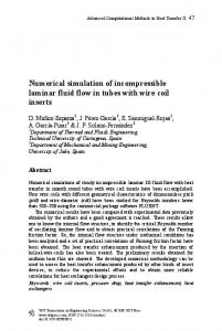
Collision Detection Figure 1 shows the three different possible cases that the collision detection has to deal with. Because fine particles can travel several lattice cells into or even across coarse particles during a single time step, it is necessary to search for fine-coarse particle collisions along the trace of each fine particle at every time step, which can be very time consuming for many particles.

Figure 1. Three possible fine-coarse particle collision types. The fine particle velocity increases from left (a) to right (c). The collision detection is separated into two subsequent steps. First, the fine particle trace, which is described by real world coordinates, i.e. floating-point numbers, has to be mapped onto the LBM lattice, which is described by integer values. This process is called voxelization as lattice cells are also named voxels. Most voxelization algorithms only treat integer-based geometries [12] as input since they were developed for scan-conversion purposes. Hence, they are not applicable for our purposes, as we are dealing with floating-point input geometries. Our collision detection algorithm transforms lattice cells to geometric objects based on floating point numbers and identifies trace-object intersections based on a standard ray-tracing method. This method leads to a unique voxel representation of each fine particle trace. The second step of the collision detection algorithm detects coarse particle boundary cells along the voxelized trace starting at the last fine particle position 1 . The firstly detected boundary cell is the collision cell. The preceding cell, meaning the fluid cell neighboring the collision cell, is provided during the deposition step as the preferred fine particle deposition site.

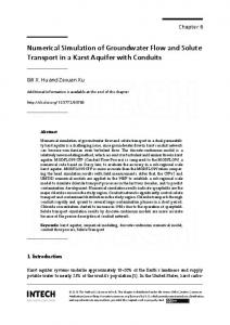
Deposition Step The deposition step converts a moving fine particle to an internal solid boundary condition in the LBM simulation, thereby modeling the riverbed clogging process. Hence, dynamic interstitial flow path patterns can be simulated, which is a superior objective of our research. The preferred deposition site is determined during the collision step, but is not necessarily the actual deposition site. Neighboring sites can also be chosen in order to achieve a more realistic deposition pattern. In the current implementation all fine-coarse particle collisions lead to deposition of fine particles at the preferred deposition site. Although this assumption may only be valid for very special hydraulic situations, resulting deposition patterns can be used as indicators for further investigations with more complex deposition models. Moreover, the deposition step does not consume any computational resources, since no additional calculations are necessary. SIMULATIONS WITH FINE SEDIMENT INFILTRATION Model Schematization A packing structure, representing a virtual riverbed, has been generated using a digital packing algorithm [13]. The domain size is 1003 lattice cells. The lattice spacing is 1 mm in physical units, and the time step = 0.02 s. The flow velocity at the inlet boundary is = 0.1 m/s for = 0.0 m/s for cells below packing height. The outlet lattice cells above packing height and boundary is placed on the y-z-plane opposite to the inlet boundary, thereby introducing current = 0.1 m/s on the domain. along the x-axis. The top boundary also imposes a flow velocity The bottom boundary is modeled via a no-slip condition; all other boundaries are periodic = 0.62 mm enter the domain normally distributed boundaries. Fine particles with = 6⁄ from the top and inlet boundary. Due to a predefined sedimentation velocity of = 0.1 m/s, particles sink to the bottom and collide/deposit on the coarse particle packing structure. The simulation runs for 3000 time steps, which is one minute in real time. In simulation (I) the particle addition rate is 5 and in simulation (II) 500 particles per second, respectively. Results The initial packing structure is illustrated in Figure 2a-b and the results of two simulations are illustrated in Figure 2c-f. The porosity , which is defined as the ratio of pore volume to total sample volume decreases during the simulation from 0.5 at the initial state to 0.498 and 0.442, respectively. Although 30,000 particles were simulated in (II), for which the collision detection algorithm has to be evaluated at every time step individually, no remarkable increase in computation time could be noticed.

Initial state

Simulation (I)

Simulation (II)

(a)

(c)

(e)

(b)

(d)

(f)

Figure 2. Packing structures (a, c, e) and cross sections (b, d, f) made of even spheres. Grey particles represent coarse sediment particles and black particles represent fine sediment particles. Volume above packing height has been removed due to simplicity. (a-b): no fine particle deposits, = 0.500. (c-d): after 1 minute of fine particle rain (addition rate: 5 particles per second), = 0.498. (e-f): after 1 minute of particle rain (addition rate: 500 particles per second), = 0.442. DISCUSSION Our results show that fine particle movement in a complex flow field can be simulated even with high numbers of fine particles. The LBM flow model confirms promising features of the TRT collision model, such as good accuracy of the results, even in complex porous geometries, and very good parallel performance. Fine-coarse particle collisions are reliably detected even with high fine particle sedimentation velocities. External riverbed clogging (deposition of fine sediments on the topmost layer of the riverbed) can be simulated for a limited number of fine particles. Anyway, the results of simulation (II) show unnatural tower-like fine particle deposition patterns. These patterns result from the deposition step, which assumes that a fine particle deposits exactly where it collides with the packing structure, i.e. at the preferred deposition site provided by the collision detection step. The penetration of the upper part of the packing structure will become unlikely if horizontal components of the flow velocity increase. Fine particles will more often deposit after horizontal collisions which may lead to external clogging in an early infiltration state.

CONCLUSION The collision detection showed good performance in terms of computational efficiency. To avoid tower-like deposit growth, the actual deposition location of fine particles should be chosen more carefully. The effect of horizontal deposition can be avoided by applying different deposition treatments for horizontal and vertical collision. The implementation of a remobilization step, preferably based on an LBM-flavored force balance, is still pending. REFERENCES [1] C. Godenschwager, F. Schornbaum, M. Bauer, H. Köstler, und U. Rüde, „A Framework for Hybrid Parallel Flow Simulations with a Trillion Cells in Complex Geometries“, in Proceedings of SC13: International Conference for High Performance Computing, Networking, Storage and Analysis, New York, NY, USA, 2013, S. 35:1–35:12. [2] U. Frisch, B. Hasslacher, und Y. Pomeau, „Lattice-Gas Automata for the Navier-Stokes Equation“, Phys. Rev. Lett., Bd. 56, Nr. 14, S. 1505–1508, Apr. 1986. [3] X. He und L.-S. Luo, „A priori derivation of the lattice Boltzmann equation“, Phys. Rev. E, Bd. 55, Nr. 6, S. R6333–R6336, Juni 1997. [4] X. He und L.-S. Luo, „Theory of the lattice Boltzmann method: From the Boltzmann equation to the lattice Boltzmann equation“, Phys. Rev. E, Bd. 56, Nr. 6, S. 6811, 1997. [5] M. Junk und A. Klar, „Discretizations for the Incompressible Navier–Stokes Equations Based on the Lattice Boltzmann Method“, SIAM J Sci Comput, Bd. 22, Nr. 1, S. 1–19, Jan. 2000. [6] P. Lallemand und L.-S. Luo, „Theory of the lattice Boltzmann method: Dispersion, dissipation, isotropy, Galilean invariance, and stability“, Phys. Rev. E, Bd. 61, Nr. 6, S. 6546–6562, Juni 2000. [7] X. He, Q. Zou, L.-S. Luo, und M. Dembo, „Analytic solutions of simple flows and analysis of nonslip boundary conditions for the lattice Boltzmann BGK model“, J. Stat. Phys., Bd. 87, Nr. 1–2, S. 115–136, Apr. 1997. [8] I. Ginzburg und D. d’ Humières, „Multireflection boundary conditions for lattice Boltzmann models“, Phys. Rev. E, Bd. 68, Nr. 6, S. 066614, Dez. 2003. [9] C. Pan, L.-S. Luo, und C. T. Miller, „An evaluation of lattice Boltzmann schemes for porous medium flow simulation“, Comput. Fluids, Bd. 35, Nr. 8–9, S. 898–909, Sep. 2006. [10] D. d’ Humières, „Generalized lattice Boltzmann equations“, in Rarefied gas dynamics: theory and simulations, American Institute of Aeronautics and AstronauticsAmerican Institute of Aeronautics and Astronautics, 1992, S. 450–458. [11] D. d’ Humières, „Multiple–relaxation–time lattice Boltzmann models in three dimensions“, Philos. Trans. R. Soc. Lond. Ser. Math. Phys. Eng. Sci., Bd. 360, Nr. 1792, S. 437–451, März 2002. [12] D. Cohen-Or und A. Kaufman, „3D line voxelization and connectivity control“, Comput. Graph. Appl. IEEE, Bd. 17, Nr. 6, S. 80–87, 1997. [13] X. Jia und R. A. Williams, „A packing algorithm for particles of arbitrary shapes“, Powder Technol., Bd. 120, Nr. 3, S. 175–186, 2001.