Numerical simulations of fluid-structure interactions in single-reed

Numerical simulations of fluid-structure interactions in single-reed mouthpieces Andrey Ricardo da Silvaa兲 and Gary P. Scavone Computational Acoustic Modeling Laboratory, Schulich School of Music, McGill University, Montreal, Quebec, Canada

Maarten van Walstijn Sonic Arts Research Centre, School of Electronics, Electrical Engineering, and Computer Science, Queen’s University Belfast, Belfast, United Kingdom

共Received 23 April 2007; revised 18 June 2007; accepted 21 June 2007兲 Most single-reed woodwind instrument models rely on a quasistationary approximation to describe the relationship between the volume flow and the pressure difference across the reed channel. Semiempirical models based on the quasistationary approximation are very useful in explaining the fundamental characteristics of this family of instruments such as self-sustained oscillations and threshold of blowing pressure. However, they fail at explaining more complex phenomena associated with the fluid-structure interaction during dynamic flow regimes, such as the transient and steady-state behavior of the system as a function of the mouthpiece geometry. Previous studies have discussed the accuracy of the quasistationary approximation but the amount of literature on the subject is sparse, mainly due to the difficulties involved in the measurement of dynamic flows in channels with an oscillating reed. In this paper, a numerical technique based on the lattice Boltzmann method and a finite difference scheme is proposed in order to investigate the characteristics of fully coupled fluid-structure interaction in single-reed mouthpieces with different channel configurations. Results obtained for a stationary simulation with a static reed agree very well with those predicted by the literature based on the quasistationary approximation. However, simulations carried out for a dynamic regime with an oscillating reed show that the phenomenon associated with flow detachment and reattachment diverges considerably from the theoretical assumptions. Furthermore, in the case of long reed channels, the results obtained for the vena contracta factor are in significant disagreement with those predicted by theory. For short channels, the assumption of constant vena contracta was found to be valid for only 40% of the duty cycle. © 2007 Acoustical Society of America. 关DOI: 10.1121/1.2759166兴 PACS number共s兲: 43.75.Pq, 43.75.Ef 关NHF兴

I. INTRODUCTION

The study of the acoustical properties of single-reed instruments has followed a paradigm first proposed by Helmholtz,1 with these systems divided into linear and nonlinear components representing the instrument’s bore and mouthpiece-reed, respectively. Previous research on the resonator component has provided an extensive list of experimental and theoretical studies since the pioneering work of Bouasse.2 Much light has been shed on the behavior of this system and, consequently, many satisfactory models have been proposed. Conversely, the amount of available literature on the mouthpiece-reed component is considerably smaller and the majority of models rely on the quasistationary approximation to describe the flow behavior. That is, the flow in a mouthpiece with an oscillating reed is assumed to be equal, at any instant, to the flow in a mouthpiece with a static reed having the same configuration.3 Moreover, the flow is considered to be frictionless and incompressible. Consequently, the dependence of the volume flow U on the pressure difference across

a兲

Electronic mail: [email protected]

1798

Pages: 1798–1809

the reed ⌬p and on the reed opening h is normally described by the Bernoulli obstruction theory based on the stationary Bernoulli equation, given by UB = hw

冑

2兩⌬p兩 sgn共⌬p兲, ␳

共1兲

where w is the channel’s width and ␳ is the density of the fluid. This approach was first presented by Backus,4 whose semiempirical model was limited to low blowing pressure regimes. Years later, Worman5 presented a more complex model addressing, in further detail, phenomena such as threshold of pressure and Bernoulli forces acting on the reed. Wilson and Beavers6 coupled the previous model to an idealized cylindrical resonator. More recent models involving the same approach were developed by Fletcher,7,8 Saneyoshi et al.9 Kergomard,10 and Olivier.11 The quasistationary approximation has also been used to derive a steady viscous flow representation by Hirschberg et al.12 Their semiempirical model was based on the results obtained from the simulation of flow in a two-dimensional 共Borda兲 tube based on the theory of potential flow. They noticed that, for Reynolds numbers Re⬎ 10, two patterns of

J. Acoust. Soc. Am. 122 共3兲, September 2007 0001-4966/2007/122共3兲/1798/12/$23.00

© 2007 Acoustical Society of America

flow may occur simultaneously, depending on the ratio l / h, where l is the length of the channel and h is its height. The flow is fully detached along the channel, for short channels 共l / h ⬍ 1兲, whereas for long channels 共l / h ⬎ 3兲 the flow is reattached at a roughly fixed point, lr, measured from the channel’s entrance. They also observed that, in the case of short channels, the vena contracta factor ␣ = T j / h was approximately constant with a value ⯝0.6, where T j is the thickness of the jet formed at the detached portion of the flow. van Zon et al.13 provided an experimental validation of Hirschberg’s model using an idealized prototype of the mouthpiece with a static reed and assuming the flow to be two dimensional. They also derived a more sophisticated flow model in which the transition between fully separated to attached flow is represented by a boundary layer solution. Other stationary measurements using realistic mouthpieces have found the same flow behavior, such as those conducted by Valkering14 and by Dalmont et al.,15 in the case of clarinet, and by Maurin,16 in the case of saxophones. However, previous attempts to characterize flow in dynamic regimes,13,17 i.e., flow in a mouthpiece with a moving reed, have suggested that the stationary behavior observed by van Zon et al. is unrealistic. This is particularly evident in the case of the steadiness associated with the detachment/ reattachment phenomenon, which is strongly affected by subtle modifications of the reed channel geometry as the reed moves. The unsteadiness of the flow modulates the aerodynamic forces acting on the reed and plays an important role in the reed’s behavior. In fact, this unsteadiness is responsible for the self-sustained oscillations in systems whose acoustic coupling between the resonator and the exciter is weak or even absent. This is the case in the harmonium,18 in the accordion,19 and in the human phonatory system.20–24 Moreover, the unsteadiness of the flow can explain why small modifications in a mouthpiece geometry can correspond to enormous changes in the transient behavior and the steady-state sound of single-reed instruments.25,26 Unfortunately, the accurate quantification and visualization of a dynamic flow controlled by a moving boundary 共in this case, the reed兲 is a rather complicated task. For this reason, previous attempts to do so are limited to qualitative outcomes.13,17 Similar difficulties are found when tackling the problem with unsteady numerical flow simulations using traditional computational fluid dynamic 共CFD兲 techniques based on the continuum theory.27,28 The objectives of this paper are the presentation of a numerical model of fully coupled fluid-structure interaction in a single-reed mouthpiece in order to address the major aspects of dynamic flow and its dependency on the reed channel geometry and to verify the validity of the quasistationary theory in dynamic regimes. To accomplish that, we implement a two-dimensional dynamic model of a singlereed mouthpiece based on a hybrid numerical approach involving the lattice Boltzmann method 共LBM兲, to represent the fluid and acoustic domains, and on a finite difference scheme to resolve the distributed model of the reed with varying cross section, as proposed by Avanzini and van Walstijn.29 The main advantage of this approach consists in J. Acoust. Soc. Am., Vol. 122, No. 3, September 2007

its simplicity in providing solutions of second-order accuracy to represent the fluid-structure interaction involving a moving boundary.30 This simplicity is contrasted with the complexity and high computational demand associated with traditional CFD techniques. Furthermore, the LBM can solve the different scales associated with the flow and acoustic fields in a single calculation, thus allowing the direct representation of the acoustic-flow interaction.31 The influence of the player’s lip and the coupling of the proposed system with the instrument’s bore and player’s vocal tract is not considered in this paper. Furthermore, the contribution of aeroacoustic sources on the instrument’s sound content due to undisturbed flow will be left to future work. This paper is organized as follows: Section II describes the model by presenting the lattice Boltzmann technique used, as well as the finite difference scheme to resolve the distributed reed model and the coupling between both techniques. Section III compares the results obtained from a stationary simulation with those provided by the quasistationary theory. Section IV evaluates the characteristics of a dynamic flow in a reed-mouthpiece system without acoustic coupling for three different reed channel geometries and compares the results with those expected by the quasistationary theory. Finally, the conclusions and remarks for future investigations are presented in Sec. V. II. THE REED-MOUTHPIECE MODEL

The following describes the implementation of the twodimensional model of the mouthpiece-reed system. The mouthpiece is represented by the LBM, which includes solid static boundaries associated with the mouthpiece walls 共face, rails, and cavity walls兲 and the fluid domain, described in terms of acoustic and fluid fields. The moving boundary associated with the reed is represented by a distributed model of a clamped-free bar with varying cross section and resolved with an implicit finite difference scheme, as proposed by Avanzini and van Walstijn.29 A. The lattice Boltzmann method

The LBM is classified as a particle or nonequilibrium technique. It simulates the space-temporal evolution of fluidacoustic systems based on a time-space discretization of the Boltzmann equation, known as the lattice Boltzman equation 共LBE兲 关see Eq. 共2兲兴. Xe and Luo32 have demonstrated that the Navier-Stokes and continuity equations can be fully recovered from the LBE for low Mach numbers, namely 共Ma⬍ 0.2兲, by applying the Chapman-Enskog expansion, thus providing a physical validity for the method. Detailed descriptions of the LBM are provided by Succi33 and Gladrow.34 The LBE controls two essential operations: advection and collision of fluid particles. These particles are described in terms of velocity distribution functions and can propagate in a discrete set of directions within the lattice. In this paper we use an isothermal two-dimensional model known as D2Q9, after Qian et al.35 In this sense, the lattice grid is represented by squared two-dimensional lattice da Silva et al.: Dynamic flow in single-reed mouthpieces

1799

The two main operations, namely, advection and collision, are controlled by the LBE,

1 f i共x + ci⌬t,t + ⌬t兲 − f i共x,t兲 = − 共f i − f iM 兲, ␶ FIG. 1. The squared grid for the D2Q9 lattice Boltzmann model.

cells containing nine sites each 共eight propagation directions and one rest site兲, as depicted in Fig. 1. Each cell connects to eight neighbor cells by the unity vectors ci, where i = 1 , 2 , . . . , 8, indicates the propagation direction associated with each site. The null vector c0 is associated with a nonpropagating site and plays an important role in improving the accuracy of the model by removing the unphysical velocity dependency of pressure.36

冦冋

冋

9 3 ␳⬘⑀i 1 + 3ci · u⬘ + 共ci · u⬘兲2 − u⬘2 2 2 f iM = 4 2 2 ␳⬘ − u⬘ 9 3

册

册

with ⑀1 = ⑀2 = ⑀3 = ⑀4 = 1 / 9 and ⑀5 = ⑀6 = ⑀7 = ⑀8 = 1 / 36. The left-hand side of Eq. 共2兲 represents the advection operation and determines the diffusion of the distribution functions f i over the lattice grid. The right-hand term determines the rate at which f i change due to intermolecular collisions between particles. This term is defined by a simplified collision function, known as BGK, after Bhatnagar, Grass, and Krook,37 which is controlled by a single relaxation time ␶ for all the advection directions i. This process, known as relaxation, forces f i toward equilibrium and restitutes the viscosity of the fluid, recovering its nonlinear form whereby the continuity and Navier-Stokes equations are satisfied. The local macroscopic variables ␳⬘ and u⬘ are obtained in terms of moments of the local distribution functions f i by

␳⬘共x,t兲 = 兺 f i共x,t兲, i

where f i is the distribution function associated with the propagation direction i at the site x⬘ and time t⬘. ␶ is the relaxation time or collision period, which acts to control the kinematic viscosity of the fluid, and f iM is the equilibrium distribution function for direction i, which depends on the local fluid velocity u⬘共x⬘ , t⬘兲 and local fluid density ␳⬘共x⬘ , t⬘兲. Here and in the following, variables indicated with a prime are adimensional. The general expressions of the equilibrium function f iM associated with the D2Q9 model are

for i = 1,2, . . . ,8 for i = 0

␳⬘共x,t兲u⬘共x,t兲 = 兺 f i共x,t兲ci .

共4兲

i

共2兲

冥

共3兲

B. The mouthpiece model

The mouthpiece model was implemented in a lattice grid containing 1002⫻ 502 cells. The physical dimensions of the system are depicted in Fig. 2, as well as the dimensions of the grid. The lattice pitch was ⌬x = 4 ⫻ 10−5 m and the time step ⌬t = 6.792⫻ 10−8 s. As a matter of convenience, we have opted to use an undisturbed fluid density ␳0⬘ = ␳0 = 1.0 kg/ m3. The relaxation time ␶ was chosen to be 0.505, which implies a lattice viscosity ␯⬘ = 1.68⫻ 10−3 and a physical kinematic viscosity ␯ = 3.95⫻ 10−5 m2 / s, using c0 = 340 m / s as the reference speed of sound. Although the choice of values for ␳0 and ␯ differ considerably from those of air in normal playing conditions, the dynamic similarity with the real system is obtained by forcing Re⯝ 1200 for a maximum Ma= 0.1. These parameters also allow the two essential criteria of the lattice Boltzmann BGK model to be met: the maximum compressibility 共Ma

Other macroscopic parameters such as lattice pressure p⬘, lattice viscosity ␯⬘, and lattice speed of sound c0⬘ are obtained by expanding the LBE into the Navier-Stokes equation and are expressed by p⬘ =

␳⬘ , 3

␯⬘ =

2␶ − 1 , 6

c0⬘ =

1

冑3 .

共5兲

The adimensional lattice variables ␳⬘, p⬘, u⬘, x⬘, t⬘, and ␯⬘ can be easily related to their respective physical counterparts ␳, p, u, x, t, and ␷ by the following relations: ␳ = ␳⬘, p = ␳c20, u = u⬘c0 / c0⬘, x = x⬘⌬x, t = ⌬x共c0⬘ / c0兲t⬘, and ␯ = 共c0 / c0⬘兲⌬x␯⬘, where c0 is the physical speed of sound. 1800

J. Acoust. Soc. Am., Vol. 122, No. 3, September 2007

FIG. 2. Lattice grid representing the two-dimensional model of the mouthpiece-reed system. da Silva et al.: Dynamic flow in single-reed mouthpieces

TABLE I. Characteristics of a plastic reed 共Plasticover兲 obtained by Avanzini and van Walstijn 共Ref. 29兲. Lreed = 34⫻ 10−3 m w = 10⫻ 10−3 m ␳reed = 500 kg/ m3 Y = 5.6⫻ 109 N / m2 ␩ = 6.0⫻ 10−7 s ␥air = 100 s−1

Length Width Density Young’s modulus Viscoelastic const. Fluid damping coef.

⬍ 0.1兲 before numerical instabilities34 and a minimum grid resolution 共5.6 lattices per wavelength兲 to avoid spurious dispersion and dissipation effects associated with the numerical bulk viscosity, as described by Crouse et al.38

C. The reed model

The reed is represented as a clamped-free bar with nonuniform thickness b共x兲, constant width w, and driven by a force F共x , t兲. The partial differential equation describing the vertical displacement y共x , t兲 as a function of F共x , t兲 is given by

␳rA共x兲

冋 冉

冊

册

⳵ ⳵2y ⳵2y ⳵2 共x,t兲 + YI共x兲 1 + ␩ 共x,t兲 = F共x,t兲, ⳵t ⳵x2 ⳵t2 ⳵x2 共6兲

where x 苸 关0 , L兴 is the horizontal position, A共x兲 = wb共x兲 is the cross section, ␳r is the material density, Y is the Young’s modulus, I共x兲 is the moment of area about the longitudinal axis, and ␩ is the viscoelastic damping coefficient. Table I shows the values used in the simulation, obtained experimentally by Avanzini and van Walstijn.29 Equation 共6兲 considers only reed motion associated with flexural waves in the vertical direction and, thus, torsional and longitudinal modes are neglected. This is similar to the approach used by Chaigne and Doutaut39 to simulate xylophone bars. In our model, a term associated with the energy dissipation of the reed due to the work exerted on the surrounding fluid is neglected in Eq. 共6兲. However, this is taken into account implicitly by the fully coupled fluid-structure interaction scheme presented in Sec. II E. Equation 共6兲 is solved by performing a space-temporal discretization based on an implicit finite difference scheme described by Chaigne and Doutaut.39 This results in a matricial difference equation in which the spatial coordinate is vectorialized, y共n + 1兲 = A0 · y共n兲 + A1 · y共n − 1兲 + AF · F共n兲,

共7兲

where y共n + 1兲, y共n兲, and y共n − 1兲 represent the displacement vector at successive time instants and A0, A1, and AF are coefficient matrices. F共n兲 is a vector representing the longitudinally distributed force on the reed. The interaction between the reed and the mouthpiece lay is considered to be inelastic. This is achieved by nullifying the kinetic energy of those reed sections that collide with the mouthpiece side rail, which presents an upper boundary to the reed. The inelastic assumption for the reed/lay interaction is discussed and justified in Ref. 29. J. Acoust. Soc. Am., Vol. 122, No. 3, September 2007

D. Initial and boundary conditions

The algorithm assumes a no-slip condition of flow at the walls by implementing a bounce-back scheme proposed by Bouzidi et al.40 The bounce-back scheme works to invert the direction of propagation of a distribution function f i just before it reaches a solid boundary. This procedure creates a null fluid velocity at the walls and provides second-order accuracy to represent viscous boundary layer phenomena. The problem of a moving boundary, the reed, within the lattice is tackled by using an interpolation scheme proposed by Lallemand and Luo.30 This technique preserves secondorder accuracy in representing the no-slip condition and the transfer of momentum from the boundary to the flow. One constraint of this approach is the velocity limit defined by Ma⬍ 0.5, Ma= ub / c0, ub being the velocity of the boundary. However, such a limitation does not represent a problem in our simulation because it corresponds to values of velocity much higher than those found for reeds at normal playing conditions. The mean flow is initiated by using a fairly well known technique in CFD called absorbing boundary conditions 共ABC兲. This technique has been adapted to LBM by Kam et al.41 and consists in using a buffer between the fluid region and the open boundary to create an asymptotic transition toward a target flow defined in terms of target distribution functions f Ti . This is done by adding an extra term to Eq. 共2兲 to represent the transition region, 1 f i共x + ci⌬t,t + ⌬t兲 − f i共x,t兲 = − 共f i − f iM 兲 − ␴共f M − f Ti 兲, ␶ 共8兲 where ␴ = ␴m共␦ / D兲 is the absorption coefficient, ␴m is a constant, normally equal to 0.3, is the distance measured from the beginning of the buffer zone, and D is the width of the buffer. The f Ti is constant and can be obtained in the same manner as f iM using Eq. 共3兲, where the local velocity u⬘ and local density ␳ are replaced by the desired target flow uT and target density ␳T, respectively. Another desired feature of this technique is the anechoic characteristic that avoids any reflection or generation of spurious waves at the open boundaries. 2

E. Numerical procedures

Seven different operations are executed at every time step in order to couple the lattice Boltzmann model with the finite difference scheme. The sequence of operations is depicted as a flowchart in Fig. 3. Before the simulation begins, the initial conditions associated with the fluid and reed variables are set and the definition of solid boundaries within the lattice are defined. The reed variables such as displacement y共x , 0兲, velocity y˙ 共x , 0兲, and force F共x , 0兲 are set to zero, as well as the variables associated with the fluid domain, such as the local fluid velocities u. The initial fluid variables are used to define the initial distribution functions based on Eq. 共3兲, so that, in the first time step f i = f iM . The flow is started by prescribing a target pressure difference at the ABC layer, T 兲c20, where the indexes “in” and defined as ⌬pT = 共␳Tin − ␳out da Silva et al.: Dynamic flow in single-reed mouthpieces

1801

simple bounce-back scheme, proposed by Bouzidi et al.40 Otherwise, f i are replaced by values calculated using the moving boundary scheme proposed by Lallemand and Luo.30 In this case, the calculation of the new f i requires the actual values of y˙ 共x , t兲 in order to take into account the transfer of momentum from the reed to the flow; 共e兲 determine new values of u⬘ and ␳⬘ using Eq. 共5兲; 共f兲 evaluate the new distributed force F共x , t兲 on the reed model based on local lattice pressures across the reed boundary; and 共g兲 calculate the reed’s new position y共x , t兲 and velocity y˙ 共x , t兲.

III. QUASISTATIC MODEL

The following compares the results obtained for a stationary simulation 共static reed兲 using the model described in Sec. II with the results provided by the quasistationary approximation for two-dimensional flows in single-reed mouthpieces with constant channel cross section, as proposed by van Zon et al.13 The model was based on the results from a stationary measurement involving an idealized twodimensional prototype of the mouthpiece-reed system. Similar measurements using real mouthpieces have found identical results and were conducted by Valkering14 and Dalmont,15 in the case of a clarinet, and by Maurin,16 for the saxophone.

A. Overview of the analytical model

FIG. 3. Flowchart of the integrated algorithm.

“out” indicate inlet and outlet, respectively. The values of ⌬pT depend on the type of simulation being conducted and are described in the next sections of this paper. With respect to the flowchart in Fig. 3, the following operations take place after the initial conditions are set: 共a兲 calculate the relaxation functions f iM ’s using Eq. 共3兲; 共b兲 propagate f i to all directions, ignoring the presence of predefined solid boundaries and perform their relaxation based on Eq. 共2兲; 共c兲 find the lattice positions of f i that have crossed solid boundaries during the propagation step in 共b兲; 共d兲 replace f i found by the previous operator with new values based on two different interpolation strategies: f i at crossed static boundaries are replaced by values calculated using the 1802

J. Acoust. Soc. Am., Vol. 122, No. 3, September 2007

Hirschberg et al.12 derived a semiempirical analytical model for the viscous steady flow in a two-dimensional single-reed mouthpiece channel with constant height. The model was based on the numerical study of a twodimensional channel 共Borda tube兲 using a potential flow scheme. They observed two types of flow for Reynolds numbers Re⬎ 10共Re= U / w␷兲, depending on the ratio between the channel height h and its length l. In both cases, a jet is formed at the sharp edges of the channel’s entrance. For small ratios 共l / h 艋 1兲, the jet does not reattach along the channel walls, whereas, for high ratios 共l / h ⱖ 3兲, the jet reattaches at a fixed point lr ⯝ h measured from the channel’s entrance. Thus, in the case of short channels, the flow is described by the Bernoulli equation 关Eg. 共1兲兴 scaled with a constant vena contracta factor ␣, whereas, in the case of long channels, the detached segment is represented by the Bernoulli flow and the reattached part is represented by the Poisseuille flow. These results were confirmed experimentally by van Zon et al.13 who derived a more accurate steady flow model in which the transition between fully separated to Poisseuille flow is described by a boundary layer flow. In this case, the velocity profile u共x , y兲 within the boundary layer of thickness ␦共x兲 is assumed to increase linearly with the distance y from the wall. Similar to the model proposed by Hirschberg et al., the flow in short channels 共l / h 艋 1兲 is given by da Silva et al.: Dynamic flow in single-reed mouthpieces

U = ␣UB ,

共9兲

where UB is the Bernoulli flow given by Eq. 共1兲 and ␣, 0.5 艋 ␣ 艋 0.61 is the constant vena contracta factor whose value depends on the external geometry of the mouthpiece. For long channels 共l / h ⱖ 4兲 and ␦共l兲 ⬎ ␦c, where ␦c is the critical boundary layer thickness, van Zon et al. describe the volume flow by

␯w 共lc − lr兲. ch

U=

共10兲

The term 共lc − lr兲 is the length of the transition between fully separated flow to Poisseuille flow, given by

冋 冑

lc − lr 12c共1 − ␦*兲2 = 1− l − lr 24c − 1

1−

册

h4共24c − 1兲⌬p , 72␳␯2共l − lr兲2共1 − ␦*兲2 共11兲

where ␦* is the generalization of the critical boundary layer thickness ␦c for a channel of arbitrary height h, expressed by

␦* = and c=

␦c h

=

冉 冑冊

4 1− 9

冋

5 = 0.2688 32

册

1 5␦* 4␦* + 9 ln共1 − ␦*兲 + = 0.01594. 6 1 − ␦*

共12兲

共13兲

B. Stationary results

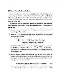
The stationary simulations were conducted for different cases involving geometries with the same characteristics as that shown in Fig. 2, but with different channel profiles as depicted in Fig. 4. For each geometry, different steady-state values of U are achieved by prescribing different target pressure values ⌬pT from 0 to 9 kPa. The simulations used the same characteristics described in Sec. II in terms of initial and boundary conditions, lattice discretization, and fluid properties. However, in this case the reed is maintained fixed 共or static兲 throughout the simulations. Figure 5共a兲 presents the numerical results obtained for the three cases in terms of vena contracta factor ␣ = U / UB as a function of the modified Reynolds number proposed by van Zon et al.13 These results are compared with those predicted by the quasistationary model presented in the previous section. For short channels, the values of ␣ were chosen to represent two geometry cases, namely, a slit in an infinite wall and a tube with sharp edges 共Borda tube兲. According to potential flow theory,42 ␣ is determined by the turning angle of the upstream flow into the channel, which depends on the characteristics of the external geometry. For the slit in an infinite wall, one finds ␣ = 0.61, whereas for the Borda tube ␣ = 0.5. Therefore, in the case of a short single-reed mouthpiece channel 共l / h 艋 1兲, one should expect an intermediate value between the two extreme cases, i.e., 0.5艋 ␣ 艋 0.61. Figure 5共b兲 plots the same simulation results in terms of volume flow U as a function of the pressure difference ⌬p and compares that with the theory provided for short and long channels as presented in Sec. III A. J. Acoust. Soc. Am., Vol. 122, No. 3, September 2007

FIG. 4. Different reed channel profiles used in the simulation: 共a兲 L / h = 1, 共b兲 L / h = 4, and 共c兲 L / h = 4 with a chamfer.

In general, Figs. 5共a兲 and 5共b兲 show that the results obtained for geometries 1, 2, and 3 agree very well with the theory presented in Sec. III A. However, Fig. 5共a兲 shows that the result for geometry 1 is in considerable disagreement for h Re/ 共l − s兲 ⬍ 60 when compared with the limits provided by the theory for short channels and fully detached flow 共0.5 艋 ␣ 艋 0.61兲. This type of disagreement is commonly reported in the literature and is attributed to the influence of viscous effects at low Reynolds numbers, as described by Durrieu et al.43 and Blevins.44 Curiously, the results obtained for geometry 2 are very similar to those found for geometry 3 and agree very well with those predicted by the theory for long channels 关Eq. 共10兲兴, despite the fact that geometry 3 has a rather diverging channel profile due to the presence of the chamfer. The flow profiles were found to be roughly constant for all geometries. In the first geometry, the flow remained fully separated for Re⬎ 30, whereas in geometries 2 and 3 the flow separated at the beginning of the channel and reattached at lr ⯝ 2h for Re⬎ 60. IV. DYNAMIC RESULTS

The goal of the following is to investigate the main aspects of the fluid-structure interaction in dynamic regimes by using the same geometries investigated in Sec. III 共Fig. 4兲. We also intend to substantiate the validity of quasistationary theory by evaluating the main assumptions associated with da Silva et al.: Dynamic flow in single-reed mouthpieces

1803

For all three cases, we use the same initial and boundary conditions described in Sec. II. The flow is initiated by prescribing ⌬pT = 5 kPa. This value corresponds to a middle point between the threshold of oscillation and the maximum pressure found for a clarinet mouthpiece.15 It must be stressed that the ABC scheme used at the inlet and outlet of the system 共Fig. 2兲 provides a complete anechoic behavior, which avoids any sort of acoustic coupling between the reed and the upstream and downstream chambers. Therefore, the reed can only move if an aerodynamic force FB exists due to flow detachment with an ensuing reattachment.25 This aerodynamic force can explain the movement of the reed during the transient state of the flow but its existence alone is, however, insufficient to explain a self-sustained oscillatory regime. This can only happen when the net energy exchanged between the flow and the reed during one duty cycle is positive: E = 兰T0 FB · y˙ tip ⬎ 0, where FB is the space averaged aerodynamic force on the reed and y˙ tip is the velocity of the reed measured at its tip. In other words, the amount of energy absorbed by the reed from the flow during one duty cycle has to be greater than the energy imparted to the flow by the reed. As explained by Hirschberg,25 in the absence of acoustic coupling, a positive net energy after one duty cycle is possible due to several reasons: 共a兲 the difference in the reed channel geometry between opening and closing phase; 共b兲 the inertia of the flow in the channel;18 and 共c兲 variability of the separation/reattachment point behavior.21 A. General results FIG. 5. Comparison between theory and numerical results for a stationary reed: 共a兲 Vena contracta factor as a function of the modified Reynolds number and 共b兲 pressure difference across the reed channel as a function of the volume flow.

the steadiness of the flow reattachment point and steadiness of the vena contracta factor when the oscillation of the reed is taken into account.

Figure 6 depicts the time histories associated with displacement of the reeds measured at their tips for all geometries. The self-sustained oscillation regime is achieved for all geometries in Fig. 4. The long channel geometries depicted in Figs. 4共b兲 and 4共c兲 present very similar behavior with high oscillation amplitudes, which forces the tip of the reed to close the channel completely. For the geometry with the short channel 关Fig. 4共a兲兴, the reed oscillation is roughly

FIG. 6. Time histories of the reed displacement measured at the tip for different channel geometries.

1804

J. Acoust. Soc. Am., Vol. 122, No. 3, September 2007

da Silva et al.: Dynamic flow in single-reed mouthpieces

sinusoidal and the average value of the tip displacement y tip ⯝ 8.0⫻ 10−4 m. Long-channel geometries present similar oscillation periods that are ⯝6.5% shorter than those found for the short-channel geometry. This vibratory behavior at a frequency close to the reed’s first natural frequency f 0 was expected, given the absence of acoustic coupling between the reed and the downstream and upstream cavities. Further analysis was carried out by investigating the dynamic characteristics of one single oscillation period. The selected duty cycles are related to the sixth oscillation period of each case and are indicated between dashed lines in Fig. 6. Figure 7共b兲 shows the normalized energy flows E˙ = FBy˙ tip as a function of time in terms of fraction of one duty cycle. The negative areas indicate transfer of energy to the flow due to the work of the reed. They take place during the phases associated with the opening of the reed, as shown in Fig. 7共a兲. Conversely, the positive areas in Fig. 7共b兲 take place when the reed is closing and represent the energy absorption by the reed due to flow work. In the regions of negative energy flow, y˙ tip and FB are out of phase but become in phase as the reed starts to close again. In all cases, the shift from negative to positive energy flow also coincides with the maximum volume flow U, shown in Fig. 7共c兲. These results present the same behavior found in the experiments conducted by Thomson23 for an idealized model of the human larynx. The high amplitudes of oscillation found in the case of long-channel geometries are explained by the higher ratios between absorbed E+ and lost energy E− during one cycle, as shown in Table II. The excess of energy given to the reed is dissipated internally by the viscous damping predicted by the third term on the right-hand side of Eq. 共6兲 and by the inelastic collision of the reed against the side lays of the mouthpiece. Furthermore, Fig. 7共b兲 shows that the reeds in the long-channel geometries start to receive energy from the flow at 0.6 T of the duty cycle, which represents a delay of 0.13 T compared to the short channel geometry. This is due to a higher flow inertia caused by larger fluid volume within long channels and due to the effect of flow driven by the moving reed, as will be discussed later in this paper. Table II presents some aspects related to the oscillation frequencies achieved by each geometry, as well as aspects related to the energy exchange between the flow and the reed. Figure 8 provides a better understanding of the results presented in Figs. 7共a兲–7共c兲 by depicting snapshots of the normalized velocity field unorm = 共u2x + u2y 兲1/2 / max共ux兲 in the mouthpiece models, taken at four different instants within the same duty cycle. In all cases, a jet is formed at the channel’s entrance as the reed starts to open. At this point, the jet rapidly adheres to the rail tip but remains detached elsewhere. This situation continues until the gradient of pressures between the jet and the reed is enough to force the jet to attach to the reed’s surface. The gradient is originated by the entrainment of flow between the jet and the reed wall due to viscous momentum transfer and it is proportional to the downstream volume flow. This phenomenon, known as the Coanda effect, plays J. Acoust. Soc. Am., Vol. 122, No. 3, September 2007

FIG. 7. Oscillation characteristics as function of time in terms of fraction of one duty cycle: 共a兲 channel aperture, 共b兲 normalized energy flow, and 共c兲 volume flow.

an important role in the self-sustained oscillations in vocal folds20–24 and in reed instruments such as the accordion19 and the harmonium.18 During the opening stage the volume flow U in the short channel accelerates earlier into the mouthpiece chamber. In fact, for the same channel aperture y tip, the volume flow into the short channel is much higher than that into the longda Silva et al.: Dynamic flow in single-reed mouthpieces

1805

TABLE II. Aspects of dynamic flow in the different channel profiles.

Geometry 1 Geometry 2 Geometry 3

L/h

f共Hz兲

f / f0

E

兩E+ / E−兩

1 4 4

1760.3 1877.2 1855.7

1.00 1.07 1.06

120.28 188.59 179.30

1.10 1.24 1.22

channel geometries, as shown in Figs. 7共a兲 and 7共c兲. The early acceleration provides the necessary pressure gradient for the jet to detach from the rail tip and adhere on the reed at ⯝0.5 T, in contrast with the long channel geometries in which the same phenomenon happens at ⯝0.7 T, as depicted in Fig. 8. The separation/adhesion phenomenon is confirmed by the determination of the skin friction based on the shear stress on the reed surface. As already mentioned, there are two explanations for the early volume acceleration in the case of the short channel. First, the fluid volume within the channel has a reduced inertia. The second reason is attributed to the effect of the flow driven by the reed Uwall. This is because, in the case of a dynamic regime, the effective volume flow can be expressed by U = U⌬p + Uwall, where U⌬p is the flow driven by the pressure difference ⌬p across the reed channel. Thus, during the

opening stage the reed exerts work on the flow by pulling it out of the mouthpiece chamber in the upstream direction, which means that U⌬p and Uwall are out of phase. In short channels, the influence of Uwall on the effective flow U is much smaller than in the case of long channels, which explains the early acceleration. The effect of Uwall also becomes significant at instants near the complete closure of the channel 共0.9T 艋 t 艋 1兲. During this period, U⌬p and Uwall are in phase and Uwall may become higher than U⌬p, which could explain the considerable unsteadiness of the flow at this fraction of the duty cycle. This phenomenon has been reported by Deverge et al.45 in the case of experiments involving prototypes of the human glottis. In their observations, however, the effect of Uwall seems to be more evident in channels with constant

FIG. 8. 共Color online兲 Snapshots of the velocity field for different instants within the same duty cycle: 共a兲 L / h = 1, 共b兲 L / h = 4, and 共c兲 L / h = 4 chamfered. 1806

J. Acoust. Soc. Am., Vol. 122, No. 3, September 2007

da Silva et al.: Dynamic flow in single-reed mouthpieces

height. This fact contrasts with our case in which the reed channel becomes divergent near the closure stage. Furthermore, the aerodynamic force FB caused by the pressure gradient increases when the jet attaches to the reed and becomes proportional to the attachment length. This explains the higher oscillation amplitudes in geometries 2 and 3. The increase in FB acts to decelerate the reed until it stops. At this point, y˙ tip and FB become in phase and the reed starts to receive energy from the flow. The stronger FB in long channels also explains the positive pitch shift in these geometries, because a stronger FB forces the reed to close more rapidly.

B. Discrepancy from the quasistationary predictions

The snapshots of flow during one duty cycle depicted in Fig. 8 show some fundamental deviations between the quasistationary assumptions and the numerical results regarding the detachment/adhesion phenomenon. In the case of the short channel geometry, Fig. 8共a兲, the constant fully separated flow assumed in the quasistationary theory has not been observed. In fact, for the first half of the duty cycle the flow is detached from the reed but remains attached to the rail tip. For the second half of the duty cycle the flow attaches to both reed and rail tip. The results for geometries 2 and 3, Figs. 8共b兲 and 8共c兲, are very self-similar. The presence of a chamfer in geometry 3 did not play a significant role on the stability of the attachment phenomenon. In those cases, the flow remains detached from the reed for nearly ⯝70% of the duty cycle. At ⯝0.7 T, the flow adheres to the reed and gradually detaches from the rail tip until the complete channel closure. This pattern contrasts with the theory, which assumes a constant separation region between the channel’s entrance and lr = 2h and full attachment of the flow afterwards. As expected, the numerical results for the vena contracta factor also diverge considerably from the theoretical predictions. Figure 9 depicts the comparison between numerical and theoretical values for ␣ along one duty as a function of the modified Reynolds number proposed by van Zon et al. The hysteresis observed for all cases in Fig. 9 agrees qualitatively with that found in a dynamic flow measurement conducted by van Zon et al.13 The hysteresis observed in the short channel geometry 关Fig. 9共a兲兴 is much smaller than that observed in the remaining cases 关Figs. 9共b兲 and 9共b兲兴. This is probably due to a less significant influence of the flow driven by the reed Uwall, as previously discussed. Furthermore, the flow adhesion segment is much shorter in the case of geometry 1, which minimizes the contribution of shear dissipation on the hysteresis. Figure 10 depicts the numerical values of ␣ as a function of time in terms of fraction of a duty cycle. For the short channel, the values of ␣ remain constant for only 35% of the duty cycle, namely 0.50 T 艋 t 艋 0.85 T. The values of ␣ become very unstable as the reed approaches the closed position. As already discussed, this characteristic is attributed to the effect of Uwall, which becomes higher than the flow driven by the pressure difference across the reed channel. J. Acoust. Soc. Am., Vol. 122, No. 3, September 2007

FIG. 9. Numerical and theoretical results for the vena contracta factor as function of the modified Reynolds number: 共a兲 geometry 1, 共b兲 geometry 2, and 共c兲 geometry 3.

V. CONCLUSIONS

We propose a numerical technique based on the lattice Boltzmann and finite difference methods to represent the problem of fully coupled fluid-structure interaction in single reed mouthpieces. The model provides second-order accuracy at representing boundary layer phenomena and was used to evaluate the behavior of three different reed channel geometries in two types of regimes, namely, stationary and dynamic. The stationary results agree very well with those predicted by the quasistationary theory, in terms of volume flow da Silva et al.: Dynamic flow in single-reed mouthpieces

1807

dynamic flow in single-reed mouthpieces and its dependency on the characteristics of the reed channel geometry. More investigations are needed in order to understand the behavior of the dynamic flow when the acoustic coupling between mouthpiece-reed system and resonator is taken into account. Another interesting step could be taken in order to investigate the mechanisms of energy transfer between flow and the acoustic field, as well as the characterization of aeroacoustic sources in the mouthpiece and its contribution to the instrument’s sound content. ACKNOWLEDGMENTS FIG. 10. Numerical values for the vena contracta factor as function of time for one duty cycle.

and vena contracta factor. Furthermore, we observed the same behavior found experimentally by van Zon et al.,13 associated with the steadiness of the vena contracta factor for different Reynolds numbers, in the case of short channels, and with the steadiness of the detachment / reattachment phenomenon in long channels. However, the results obtained during the dynamic simulations are very different from those predicted by the quasistationary theory. For the short channel geometry, ␣ was found to be constant for only ⯝40% of the duty cycle, and for long channels, the values of ␣ were in stark disagreement with the quasistationary predictions. Moreover, the patterns observed in stationary measurements such as fully detached flow, in the case of short reed channels, and the twofold pattern, in the case of long channels, were not observed in the dynamic simulations. The main difference in the flow behavior between short and long channels was found to be the time taken by the flow to adhere on the reed wall within one duty cycle. This characteristic was attributed to the effect of inertia associated with different fluid volumes within the reed channel and to the flow driven by the reed. The results also show that different levels of self-sustained oscillations can be achieved in the absence of acoustic feedback due to the complexity of hydrodynamic forces acting on the reed, which supports the hypothesis proposed by Hirschberg et al.12,25 in the case of single reed mouthpieces. The two-dimensional nature of our numerical approach restricts the results to a qualitative analysis. Another limitation is associated with the lack of acoustic feedback, which neglects eventual influences of the acoustic field on the flow within the reed channel. Nevertheless, we feel it is worthwhile to focus on the aerodynamicaly oscillating situation presented in this paper. The widespread assumptions made in modeling wind instrument reeds that have been reported many times in this journal and others are based on a quasistationary assumption that itself does not take into account the influence of the acoustic field on the flow behavior. The simulations reported in this paper show that there are significant deviations from these long held assumptions that call into question the validity of the currently accepted model. These deviations might easily be obscured in the presence of acoustic feedback. Furthermore, the approach presented in this paper contributes to our understanding of the behavior of 1808

J. Acoust. Soc. Am., Vol. 122, No. 3, September 2007

The authors would like to thank Professor Luc Mogeau and the anonymous reviewers of this paper for their helpful suggestions. A.R.d.S wishes to thank CAPES 共Funding Council of the Brazilian Ministry of Education兲 for supporting his doctoral research. 1

H. L. F. Helmholtz, On the Sensations of Tone as a Physiological Basis for the Theory of Music 共Dover, New York, 1877兲. 2 H. Bouasse, Instruments à Vent (Wind Instruments) 共Blanchard, Paris, 1929兲, Vols. I and II. 3 S. S. Chen, “A general theory for dynamic instability of tube arrays in crossflow,” J. Fluids Struct. 1, 35–53 共1987兲. 4 J. Backus, “Small-vibration theory of the clarinet,” J. Acoust. Soc. Am. 35, 305–313 共1963兲. 5 W. E. Worman, “Self-sustained nonlinear oscillations of medium amplitude in clarinet-like systems,” Ph.D. thesis, Case Western Reserve University, Cleveland, OH, 1971. 6 T. A. Wilson and G. S. Beavers, “Operating modes of the clarinet,” J. Acoust. Soc. Am. 56, 653–658 共1974兲. 7 N. H. Fletcher and T. D. Rossing, The Physics of Musical Instruments 共Springer, New York, 1998兲. 8 N. H. Fletcher, “Air flow and sound generation in musical instruments,” Annu. Rev. Fluid Mech. 11, 123–146 共1979兲. 9 J. Saneyoshi, H. Teramura, and S. Yoshikawa, “Feedback oscillations in reed woodwind and brasswind instruments,” Acustica 62, 194–210 共1987兲. 10 J. Kergomard, “Elementary considerations on reed-instruments oscillations,” in Mechanics of Musical Instruments, edited by A. Hirschberg, J. Kergomard, and G. Weinreich 共Springer, Wien, 1995兲. 11 S. Ollivier, “Contribution á l’étûde des oscillations des instruments à vent à anche simple: Validation d’un modèle élémentaire 共Contribution to the study of oscillations in single-reed instruments: Validation of an elementary model兲,” Ph.D. thesis, University of Maine, Maine, 2002. 12 A. Hirschberg, R. W. A. van der Laar, J. P. Marrou-Mauriere, A. P. J. Wijnands, H. J. Dane, S. G. Kruijswijk, and A. J. M. Houtsma, “A quasistationary model of air flow in the reed channel of single-reed wind instruments,” Acustica 70, 146-154 共1990兲. 13 J. van Zon, A. Hirschberg, J. Gilbert, and A. P. J. Wijnands, “Flow through the reed channel of a single reed instrument,” in Congrs Franais d’Acoustique Sup. J. Phys. Colloque de Physique, Paris, Vol. 54, pp. 821824 共1990兲. 14 A. M. C. Valkering, “Characterization of a clarinet mouthpiece,” Technical Report No. R-1219-S, Vakgroep Transportfysica, TUE, Eindhoven, 1993. 15 J. P. Dalmont, J. Gilbert, and S. Ollivier, “Nonlinear characteristics of single-reed instruments: Quasistatic volume flow and reed opening measurements,” J. Acoust. Soc. Am. 114, 2253–2262 共2003兲. 16 L. Maurin, “Confrontation théorie-expérience des grandeurs d’entrée d’un excitateur à anche simple 共Theoretical and experimental comparisons of input variables in a single-reed oscillator兲,” Ph.D. thesis, University of Maine, Main, 1992. 17 J. Gilbert, “Étude des instruments de musique à anche simple 共A study of single-reed musical instruments兲,” Ph.D. thesis, University of Maine, Maine, 1991. 18 A. O. St-Hilaire, T. A. Wilson, and G. S. Beavers, “Aerodynamic excitation of the harmonium reed,” J. Fluid Mech. 49, 803–816 共1971兲. 19 D. Ricot, R. Causse, and N. Misdariis, “Aerodynamic excitation and sound production of a blown-closed free reeds without acoustic coupling: The da Silva et al.: Dynamic flow in single-reed mouthpieces

example of the acordion reed,” J. Acoust. Soc. Am. 117, 2279–2290 共2005兲. 20 X. Pelorson, A. Hirschberg, R. R. van Hassel, A. P. J. Wijnands, and Y. Auregan, “Theoretical and experimental study of quasisteady-flow separation within the glottis during fonation. Application to a modified two-mass model,” J. Acoust. Soc. Am. 96, 3416–3431 共1994兲. 21 B. D. Erath and M. W. Plesniak, “The occurrence of the coanda effect in pulsatile flow through static models of the human vocal folds,” J. Acoust. Soc. Am. 120, 1000–1011 共2006兲. 22 S. L. Thomson, L. Mongeau, and S. H. Frankel, “Aerodynamic transfer of energy to the vocal folds,” J. Acoust. Soc. Am. 118, 1689–1700 共2005兲. 23 S. L. Thomson, “Fluid-structure interactions within the human larynx,” Ph.D. thesis, Purdue University, West Lafayette, IN, 2004. 24 I. R. Titze, “The physics of small-amplitude oscillations of the vocal folds,” J. Acoust. Soc. Am. 83, 1536–1552 共1988兲. 25 A. Hirschberg, J. Gilbert, A. P. Wijnands, and A. M. C. Valkering, “Musical aero-acoustics of the clarinet,” J. Phys. IV 4, 559–568 共1994兲. 26 A. H. Benade, Fundamentals of Musical Acoustics 共Oxford University Press, New York, 1976兲. 27 W. Shyy, Computational Fluid Dynamics with Moving Boundaries, Series in Computational Methods and Physical Processes in Mechanics and Thermal Sciences 共Taylor and Francis, New York, 1995兲. 28 M. Liefvendahl and C. Troeng, “Deformation and regeneration of the computational grid for cfd with moving boundaries,” in Proceedings of the 45th AIAA Aerospace Science Meeting, Nevada, 2007. 29 F. Avanzini and M. van Walstijn, “Modelling the mechanical response of the reed-mouthpiece-lip system of a clarinet. 1. A one-dimensional distributed model,” Acta Acust. 90, 537–547 共2004兲. 30 P. Lallemand and L. S. Luo, “Lattice Boltzmann method for moving boundaries,” J. Comput. Phys. 184, 406–421 共2003兲. 31 X. M. Li, R. C. K. Leung, and R. So, “One-step aeroacoustics simulation using lattice Boltzmann method,” AIAA J. 44, 78–89 共2006兲. 32 X. He and L. S. Luo, “Theory of the lattice Boltzmann method: From the Boltzmann equation to the lattice Boltzmann equation,” Phys. Rev. E 56, 6811–6817 共1997兲. 33 S. Succi, The Lattice Boltzmann Equation for Fluid Dynamics and Beyond

J. Acoust. Soc. Am., Vol. 122, No. 3, September 2007

共Oxford University Press, Oxford, 2001兲. D. A. Wolf-Gladrow, Lattice Gas Cellular Automata and Lattice Boltzmann Models: An Introduction, Lecture Notes in Mathematics, Vol. 1725 共Springer, Berlin, 2004兲. 35 Y. Qian, D. d’Humires, and P. Lallemand, “Lattice BGK models for the Navier-Stokes equation,” Europhys. Lett. 17, 479–484 共1992兲. 36 Y. Qian, S. Succi, and S. A. Orszag, “Recent advances in lattice Boltzmann computing,” Annu. Rev. Comput. Phys. 3, 195–242 共1995兲. 37 P. L. Bhatnagar, E. P. Gross, and M. Krook, “A model for collision processes in gases. I. Small amplitude processes in charged and neutral onecomponent systems,” Phys. Rev. 94, 511–525 共1954兲. 38 B. Crouse, D. Freed, G. Balasubramanian, S. Senthooran, P. Lew, and L. Mongeau, “Fundamental capabilities of the lattice Boltzmann method,” in Proceedings of the 27th AIAA Aeroacoustics Conference, Cambridge, 2006. 39 A. Chaigne and V. Doutaut, “Numerical simulations of xylophones. 1. Time-domain modeling of the vibrating bars,” J. Acoust. Soc. Am. 101, 539–557 共1997兲. 40 M. Bouzidi, M. Firdaouss, and P. Lallemand, “Momentum transfer of a Boltzmann-lattice fluid with boundaries,” Phys. Fluids 13, 3452–3459 共2001兲. 41 E. W. S. Kam, R. M. C. So, and R. C. K. Leung, “Non-reflecting boundary for one-step lbm simulation of aeroacoustics,” in 27th AIAA Aeroacoustics Conference, Cambridge, MA, 2006, pp. 1–9. 42 R. H. Kirchhoff, Potential Flows, Mechanical Engineering 共CRC, New York, 1985兲. 43 P. Durrieu, G. Hofmans, G. Ajello, R. Boot, Y. Aurégan, A. Hirchberg, and M. C. A. M. Peters, “Quasisteady aero-acoustic response of orifices,” J. Acoust. Soc. Am. 110, 1859–1872 共2001兲. 44 R. D. Blevins, Applied Fluid Dynamics Handbook 共Van Nostrand Heinhold, New York, 1984兲. 45 M. Deverge, X. Pelorson, C. Vilain, P.-Y. Lagreé, F. Chentouf, J. Willems, and A. Hirschberg, “Influence of collision on the flow through in-vitro rigid models of the vocal folds,” J. Acoust. Soc. Am. 114, 3354–3362 共2003兲. 34

da Silva et al.: Dynamic flow in single-reed mouthpieces

1809