observed that directionally bi-modal wave spectra can give rise to a new ... (Lumped Triad Approximation) model proposed by Eldeberky and Battjes (1995) and.
NUMERICAL SIMULATIONS OF DIRECTIONALLY SPREAD SHOALING SURFACE GRAVITY WAVES Francoise BECQ1, Michel BENOIT1, Philippe FORGET2 ABSTRACT
The study aims at investigating the non-linear triad interaction process affecting shoaling surface gravity wave fields in shallow water areas. Attention is specifically paid to analyse the effects of these second-order non-linearities on the directional distribution of incident waves. A stochastic approach was chosen to model the triad interaction process. Three source terms have been implemented in the spectral wave model TOMAWAC developed at the Laboratoire National d'Hydraulique (LNH). The model results are compared to the laboratory data of Nwogu (1994). 1. INTRODUCTION: This work focusses to the study of the non-linear interactions between triplets of waves which occur in the nearshore zone. These non-linearities, of lower order than the four wave interactions, are usually considered as the main exchange mechanism for wave energy of an irregular wave train towards sub- (long waves) and super-harmonics (bound higher order waves) (e.g. Freilich and Guza, 1984). The strength of these near-resonant interactions is governed by the phase mismatch between the bound and free wavenumbers. As for decreasing water depth the waves tend to become non-dispersive, the phenomenon is enhanced towards the shore. The effect of the transfer of energy associated with near-resonant wave interactions is not only distortions of the frequency spectrum, but also modifications of the directional spreading of energy. Elgar et al. (1993) observed that directionally bi-modal wave spectra can give rise to a new directional peak. This implies that both collinear and non-collinear triad interactions are important. Boussinesq equations have been extensively used to establish evolution equations for the amplitudes and phases of unidirectional waves propagating over a mildly sloping bottom. The models (e.g. Freilich and Guza (1984), Madsen and Sorensen (1993)) are able to correctly reproduce the generation of harmonics. The quality of the results incited us to extend the deterministic model of Madsen and Sorensen (1993) to bidimensional situations. The model is presented in part 2. 'EDF - Laboratoire National d'Hydraulique, 6 quai Watier, 78400 Chatou, FRANCE L.S.E.E.T Universite de Toulon et du Var, BP 132, 83957 La Garde, FRANCE
2
523
524
COASTAL ENGINEERING 1998
Alternatively, stochastic (phase-averaged) models are more useful to predict the evolution of directional wave spectra. The shallow water three-waves interaction process is simulated by including a source term in the energy balance equation. From the works of Zakharov et al. (1992), Eldeberky et al. (1996) proposed a directionally coupled source term. Some misbehaviours of this non-linear model were pointed out by the authors. We studied more particularly the problem of energy conservation and the ability to generate new directional peaks (which was not demonstrated in Eldeberky, 1996). For practical applications, Eldeberky et al. (1996) recommended the use of the parametrized LTA (Lumped Triad Approximation) model proposed by Eldeberky and Battjes (1995) and Eldeberky (1996). This model has been applied in the wave propagation model SWAN developed at Delft University of Technology (Ris, 1997). The LTA model is characterised by the restriction to self-self interactions leading to a great computational efficiency. From the 2D spectral deterministic equation presented in §2, we developed a new stochastic model. To solve the classical problem of closure, we used the works of Holloway (1980) who assumes that the sum over fourth-order moments draws some contribution from third-order moments through a coupling coefficient interpreted as a broadening of the resonance condition. The three formulations for phase-averaged models are presented in part 3. They are implemented in the spectral wave model TOMAWAC developed at the LNH (Benoit et al., 1996) and they have been compared to the experimental laboratory results presented by Nwogu (1994) (§4).
2. DETERMINISTIC APPROACH: Deterministic Boussinesq (SB) model: Starting from their extended Boussinesq equations, Madsen and Sorensen (1993) derived a set of deterministic evolution equations for the amplitudes and phases of unidirectional waves propagating over a mildly sloping bottom. We extended the model to bidimensional situations by use of the 2D Boussinesq equations of Madsen and Sorensen (1992): ^ + V.P = 0 dP
(1)
2 ... -(v.p)+(?.v)— t +g(h + C)V^-\B + Uh V
6{ 2
dt)
6^
\dt) 6 2
{
' dt
dt)
J
-Bgh (Vh.v)(V£)- Bgh [V.V;)Vh- Bg/z v(v.Vf) = 0 where f is the free surface elevation, P is the depth-integrated velocity and h is the water depth. These equations include a linear parameter B which improves the dispersion properties and the shoaling mechanisms associated with the model. The optimal value B=l/15 was obtained by the authors by a fit to the reference linear shoaling coefficient predicted by the Stokes first-order theory. The standard form of the Boussinesq equations can be recovered by setting B=0.
COASTAL ENGINEERING 1998
525
The extended Boussinesq equations are combined into one single equation. For this, the partial derivative in time of the continuity equation is substracted to the partial derivative in space of the momentum equation. This leads to: L=M + N (3) where:
L = c„-gW.v? + B^v.(v(v.vc))-fs+^yv.(v^„)
(4)
M = gVh.V£+(2B+l)hVh.V£,,-5Bgh2Vh.^.fC)+-Vh.(v®(V®Pl))
(5 )
JV = V.
:{y.p)+(p.v)-
+ gVf.VC + g£V.VC
(6)
L contains the lowest order and dispersive terms, M represents the effects of slowly varying depths on the wave propagation and N models the non-linear effects due to wave coupling. Now, the equation is transformed into the spectral domain. £ is written as a discrete Fourier series: £(x,y,t)= £A„(*,)0exp[i(p) and y/ is the linear wave phase, linked to the wavenumber by the relation Vi//p = k~ (x,y). P is linked to £ through the continuity equation, so: P{x,y,t)~^cpAp{x,y)e^^\
(8)
where c is the wave phase celerity. The Fourier expressions of f and P are inserted in the equation (3). We follow for this the guideline presented by Madsen and Sorensen (1993) for ID situations. First derivatives of Ap , kp and h axe assumed to be small, and products of derivatives and higher derivatives of these quantities are neglected. After algebraic manipulations, we get, • at lowest order, the linear dispersion relation: ->- *-> A =-*- Np dt " 2 kp " " 2S,p " 2SUp " where Cg is the group velocity:
(10)
CgP=^-kP
(11)
SliP=2) and through the parameter Q characterising non-resonant interactions: Q. M3-1-2
(23)
—
"
(o3 -ft), -a>2) +Q.2
For the resonant conditions: k, -k, -£, =0 and ft). -ft), -ft), =0, the weak wave theory of Zakharov et al. (1992) assumes that £2—>0, implying: M3-1-2 =7tS(co, -co, -co2) (24) Eldeberky et al. (1996) showed by numerical simulations that the spectral source term for triad interactions results in an artificial energy decay/gain. This non-conservative feature was explained by the specification of the filter bandwidth Q. As done by Hasselmann and Hasselmann (1985) for quadruplets interactions, we exploited the basic symmetry of the triplets interactions to study more accurately the problem of energy conservation. The interaction coefficient R3i2, as well as Nil2 and /j.ll2 are invariant with respect to permutations between waves 1 and 2. So, for the collision: £, - k, - k2 = 0 ( 25 ) the changes An,, in wave action per unit time for the three wavenumbers can be expressed by: An? "•1
Atlr h
— 1
f
312
312 r^312 ^\
3
2
1 J^'^1^'^2
(26)
3
+1
An?
leading to:
^ ^ .^
[-/.) •
=
•
-f^
' r^312 ^1^3
*^2
1 ("f'f'1^'^'2
3
(27)
Vh\
( 26 ) and ( 27 ) show that, for resonant three wave interactions f} = /, + f2, only the
528
COASTAL ENGINEERING 1998
conservation of energy applies, as expected (Komen et al, 1994). Non-conservation of energy occurs for near-resonant interactions when the linear dispersion relationship is used to link the wavenumber to the frequency since /'"'(£3 )p F F + p p m k ~ V 2, p-m k p-m
F F
p
m
^
p-m,m p p i p-m m 2,p p
(47)
with Ak2 = \kp - kp_m - km | Substitution of equation (47) into (37) leads to:
(48) M2 'R",-^m
^F„F
+- c
r t - p~ P-m • °2,mKm
F„F„
r, ' P l,p-mKp-m
J
m
-P~m p
c
h
p-i"
p •
531
COASTAL ENGINEERING 1998
For its implementation in the TOMAWAC spectral wave model, the SPB source term (right hand side of (48)) is expressed in terms of the continuous frequency-directional variance density function F(f ,9). The source term may be written as: s V»eO = f f f fdM^dej• 8(eh -^+J«s(/3 -/, -f2) (49 1 J— e2" r~ fix , . v^ ' o I I )0dm2dexdej^8{eh -e^jsfa-fi +/2) where 7^'• and 7^• represent respectively the sum and difference triad interactions. The formulation is directionally coupled and allows for both collinear and non-collinear interactions.
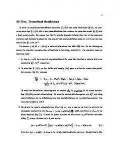
4. NUMERICAL SIMULATIONS: The three non-linear source terms presented in §3 have been implemented in the spectral wave model TOMAWAC, developed at the Laboratoire National d'Hydraulique (Benoit et al., 1996). Numerical simulations are compared to the experimental laboratory results presented by Nwogu (1994), for the propagation of crossing seas over a constant slope. Laboratory Basin description (Nwogu, 1994; Nwogu, 1993) The three-dimensional wave basin (30 m wide, 20 m long and 3 m deep) is located at the Hydraulics Laboratory, National Research Council of Canada. It is equipped with a segmented directional wave generator. Reflections at the basin sidewalls are reduced by wave energy absorbers made of perforated metal sheets. A bathymetric profile was constructed in the basin. It consists in a constant slope beach (1:25) with an impermeable concrete cover. The free surface elevation was measured along the centreline of the basin with a linear array of 23 water level gauges. Wave conditions imposed at the wave generator The incident laboratory wave spectrum at the wave generator (h = 0.56 m) is bimodal: it is composed of two sea states characterising local sea and swell components (figure 1). The frequency distributions of the sea states are described by a JONSWAP spectrum characterised by the peak period T , the significant wave height Hm0 and the peak enhancement factor y . The directional distributions are given by the cosine function: D{8)=cos2'(9-6 0)
(50)
Table 1 sums up the wave parameters of the target spectrum. Swell Hm0(m) 0.068
Local sea
s y 2>) o0o HM(.m) ?>) r 10 2.5 0.062 1.5 22 22.5 3.3 6 Table 1. Spectral wave parameters characterising the initial spectrum. J
0o o -22.5
532
COASTAL ENGINEERING 1998 variance density (m2/Hz/deg) X10 1.8 *,..-••"""
frequency
0
direction (deg)
Figure 1 : Directional wave spectrum imposed at the wave generator. Numerical results The SPZ source term was activated in the TOM AW AC simulation, with i2=0.05. The directional wave spectrum obtained in the shallow water area (h = 0.18 m) is presented on figure 2. It shows that the variance density spectrum is affected by refraction, shoaling and non-linear triad interactions. Non-linear wave-wave interactions strongly affect the frequency-directional shape of the spectrum. By collinear wave-wave interactions, energy is transferred from the swell spectral peak towards its two higher harmonics and by noncollinear interactions, energy is transferred from the two primary spectral peaks (swell and local sea) towards the component corresponding to the vector sum of the primary peak wavenumbers. Figure 3 shows a comparison between the non-linear SPZ simulation and measurements for the frequency spectrum. The results obtained with a linear simulation are also presented to point-up the effects of wave-wave interactions on the spectral shape. Figure 3 clearly demonstrates that the non-linear triads interactions cannot be neglected in the shoaling zone. As shown by Eldeberky et al. (1996), the new spectral peaks generated using the SPZ model are shifted towards lower frequencies as compared to measurements. Since the interaction condition between the three interacting waves is imposed through £>(£, — £, - £,), the negative curvature of the linear relationship implies that if £, = £, + £2, then /,