Let Ω denote a bounded open domain of R2 with boundary âΩ and let λ stand .... We can now summarize the complete time parameterized problem : find (Ï, v, ...
Numerical Solution of the Free Boundary Bernoulli Problem Using a Level Set Formulation Fran¸cois Bouchon, St´ephane Clain, Rachid Touzani Laboratoire de Math´ematiques Appliqu´ees, CNRS UMR 6620 Universit´e Blaise Pascal (Clermont–Ferrand) 63177 Aubi`ere cedex, France
Abstract We present a numerical method based on a level set formulation to solve the Bernoulli problem. The formulation uses time as a parameter of boundary evolution. The level set formulation enables to consider non connected domains. Numerical experiments show the efficiency of the method if boundary conditions are handled accurately. In particular, the case of multiple solutions is treated. R´ esum´ e Nous pr´esentons une m´ethode num´erique bas´ee sur une formulation en ensembles de niveaux pour la r´esolution du probl`eme de fronti`ere libre de Bernoulli. La formulation utilise le temps comme param`etre d’´evolution de la fronti`ere. La formulation en ensembles de niveaux permet de consid´erer des domaines non connexes. Les essais num´eriques montrent l’efficacit´e si les conditions aux bord sont prises en compte d’une mani`ere pr´ecise. En particulier, nous traitons le cas de solutions multiples.
Keywords : Free Boundary Problem, Bernoulli Problem, Level Set Formulation.
2
1
Introduction
Level set formulation of free boundary problems is widely used in scientific computing. This formulation offers indeed numerous advantages when compared with traditional front tracking techniques. In particular, it is well known that topology breakdown in free boundary evolution can not be handled by a standard front tracking method. The reader is referred for this purpose to a wide literature and, in particular, the monograph of Sethian [7] gives a very clear introduction to these methods. We consider in this paper the numerical solution method of the so-called Bernoulli problem. This problem can be considered as a typical example of a stationary free boundary problem. Its applications appear in fluid dynamics [5], optimal design [4], electromagnetics [2, 3] and various other engineering fields. The presented numerical method is based on a level set formulation of the Bernoulli problem. More specifically, since this problem is time independent we derive a simpler formulation of the method, the basic tool being an adequate extension of the propagation velocity of the unknown boundary. Let Ω denote a bounded open domain of R2 with boundary ∂Ω and let λ stand for a negative real number. We can distinguish two types of Bernoulli problems. The interior Bernoulli problem consists in seeking a subset A, with boundary ∂A, of Ω and a real-valued function u defined on Ω \ A such that : ∆u = 0
in Ω \ A,
u=0 u=1 ∂u =λ ∂n
on ∂Ω, on ∂A,
(1.1) (1.2) (1.3)
on ∂A.
(1.4)
Here, n stands for the unit normal to ∂Ω, external to Ω. The exterior Bernoulli problem consists in seeking a superset A ⊃ Ω and a function u defined on A \ Ω such that : ∆u = 0 u=1 u=0 ∂u =λ ∂n
in A \ Ω, on ∂Ω, on ∂A,
(1.5) (1.6) (1.7)
on ∂A.
(1.8)
Let us note that a theoretical study (existence, uniqueness, stability) was carried out in [1, 4]. In particular the notion of elliptic, hyperbolic and parabolic solution is defined. In view of this, we are interested in what the authors in [1, 4] call elliptic solutions. Another property that is addressed in the same paper is nonuniqueness. We shall consider this topic in numerical experiments where we exhibit some examples with multiple solutions. Numerical solution of such problems requires first defining an iterative procedure since the problem is nonlinear and then numerical approximation using a space and time discretization. For the first issue, we shall study in this paper two schemes based on a Dirichlet and a Neumann boundary condition. Advantages and drawbacks of these formulations will be compared through numerical experiments. Concerning numerical methods, we use a simple 3
Euler scheme for time integration and a finite difference scheme for space discretization, the computational domains being rectangular. We derive a modified finite difference scheme in order to accurately fit the wanted boundary. The outline of the paper is the following. In Section 2, we derive a level set formulation for both exterior and interior Bernoulli problems. For each one a Dirichlet and a Neumann formulation are given, the main issue being the choice of an ad hoc extension of the propagation velocity of the free boundary that enables defining a level set equation in the whole domain under consideration. In Section 3, we first give an iterative procedure to solve the resulting nonlinear problem and then give time and space discretization schemes and finally, Section 4 presents some numerical results.
2
The Level Set Formulation
Let us recall that a level set formulation consists in defining the unknown boundary ∂A as the level set φ = 0 of a function φ, i.e. ∂A = {x ∈ R2 ; φ(x) = 0}. In the case of the interior Bernoulli problem (1.1)–(1.4), we require that φ is positive in Ω \ A and negative in A. The case of the exterior problem (1.5)–(1.8) can be handled in the same way, i.e. φ should be positive out of A and negative in A. With such a convention, the outward normal vector of A is given by n=
∇φ . |∇φ|
Now, although problems (1.1)–(1.4) and (1.5)–(1.8) are stationary, the level set formulation requires a time evolution principle. For this, we introduce the time variable t as a parameter. The expected solution (if this one exists) being the one obtained after convergence for large time. Assume now that we have a family of boundaries (A(t))t>0 given by ∂A(t) = {x ∈ R2 ; φ(x, t) = 0}, for an unknown function φ : Ω × R+ → R. Clearly, we shall construct an iteration process, based on φ, that converges toward a solution of (1.1)–(1.4) or (1.5)–(1.8). There are at least two ways to construct such a process. Let us describe hereafter these formulations for the exterior problem.
2.1
A Neumann Formulation
Consider the time parameterized solution u(t) defined in A(t) \ Ω by : ∆u(t) = 0
in A(t) \ Ω,
u(t) = 1 ∂u(t) =λ ∂n
on ∂Ω, on ∂A(t). 4
We consider the quantity u(t) as a velocity which vanishes when A(t) coincides with the solution A. As an extension of the formulation proposed by [4], the displacement of the boundary ∂A can be obtained by considering the following equation : ∂φ + u(t) = 0 ∂t
on ∂A(t).
Another important issue in the level set approach is to extend the previous equation to the whole domain R2 \ Ω. For this end, we define the problem : ∆v(t) = 0 v(t) = 0 v(t) = u(t)
in (A(t) \ Ω) ∪ (R2 \ A(t)), on ∂Ω, on ∂A(t).
Then φ is extended to R2 \ Ω by ∂φ +v =0 ∂t
in R2 \ Ω.
We can now summarize the complete time parameterized problem : find (φ, v, u) such that ∆u(t) = 0 u(t) = 0 ∂u(t) =λ ∂n ∆v(t) = 0 v(t) = 0 v(t) = u(t) ∂φ + v(t) = 0 ∂t
in A(t) \ Ω,
(2.1)
on ∂Ω,
(2.2)
on ∂A(t),
(2.3)
in (A(t) \ Ω) ∪ (R2 \ A(t)), on ∂Ω, on ∂A(t),
(2.4) (2.5) (2.6)
in R2 \ Ω,
(2.7)
where ∂A(t) = {x ∈ R2 ; φ(x, t) = 0} and A(t) = {x ∈ R2 ; φ(x, t) < 0}. The expression “Neumann formulation” is due here to the fact that the partial problems (for given A(t)) that we shall solve iteratively (2.1)–(2.3) are actually boundary value problems that involve a Neumann boundary condition on ∂A(t).
2.2
A Dirichlet Formulation
An alternative to the previous problem is to provide the partial problem (with given domain A(t)) with a Dirichlet boundary condition. The problem consists then in seeking (φ, v, u) such
5
that ∆u(t) = 0 u(t) = 0 u(t) = 1 ∆v(t) = 0 v(t) = 0 ∂u(t) v(t) = λ − ∂n ∂φ +v =0 ∂t
in A(t) \ Ω, on ∂Ω, on ∂A(t),
(2.8) (2.9) (2.10)
in (A(t) \ Ω) ∪ (R2 \ A(t)), on ∂Ω,
(2.11) (2.12)
on ∂A(t),
(2.13)
in R2 \ Ω.
(2.14)
Naturally, Problems (2.1)–(2.7) and (2.8)–(2.14) lead to different numerical schemes that do not have the same behaviour with respect to stability and convergence.
3
Numerical Solution
We now turn to the numerical approximation of the level set problem. We shall see that some differences between the the Dirichlet and the Neumann versions ((2.8)–(2.14) and (2.1)–(2.7) respectively) are to be taken into account. We start by assuming that the free boundary A(t) evolves within a large bounded domain Λ with boundary ∂Λ. This domain can be chosen for simplicity as the square (0, 1) × (0, 1).
3.1
An iterative procedure
Since time plays the role of a parameter in this problem, we consider an iterative procedure that looks like a time integration scheme for which a parameter τ > 0 stands for a time step. Let us assume that the function φk (approximation of φ at time kτ ) is given. The boundary ∂Ak is hence the set of zeroes of the function φk . We approximate Equation (2.7) by the forward Euler scheme : φk+1 = φk − τ v k , k = 0, 1, . . . where v k is solution of the problem : ∆v k = 0
(3.1)
on ∂Ak ,
(3.2)
on ∂Ω ∪ ∂Λ.
(3.3)
k
∂u ∂n vk = 0
vk = λ −
¡ ¢ ¡ ¢ in Ak \ Ω ∪ Λ \ Ak ,
The function uk is obtained by solving the following boundary value problem : ∆uk = 0 k
u =0 uk = 1
6
in Ak \ Ω,
(3.4)
on ∂Ω, on ∂Ak ,
(3.5) (3.6)
3.2
A finite difference scheme for the Dirichlet formulation
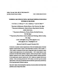
We consider a uniform mesh made of grid points (xi , yj ) = (ih, jh), 0 ≤ i ≤ n. The position of the approximate boundary ∂Ak is determined by the values of the approximation φki,j of φk (xi , yj ). Let P = (xi , yj ), and PN , PW , PE and PS stand for its four neighbor points as depicted in Figure 1. We shall also denote in the sequel by uP , uN , uS , uW and uE the values of uij , ui,j+1 , ui,j−1 , ui−1,j , ui+1,j respectively and so for φ. Note that we omitted to indicate the iteration index for the sake of conciseness. Finally, PB will denote the position of the free boundary on the line i, supposed to be located between P and PE . Here, in the case of Figure 1, we have φP φE < 0.
.... .... .... .... .... ... ... ... ... ... .. .. .. .. .. ......................................................................................................................................................................................................................................................................... ....... . . . ... ... ....... .... .... . . .... ....... .. .. ....... .. . .... .... . .... ....... . .... .... ........ .... .... .... .... .... ...... .... .... .... .... .... ..... .... .... ... .... .... .... .... .... ... ... . . . . ..... ..... . . ... ..........................................................................................................................N ............................................................................................................................................. .. .. .. . .. ... ... ... .... .... .... . .... ... . ... .... .... .... .... .... ... .. .... .... .... . .... ... . ... .... .... .... .... .... ... . . ..... ..... ..... . ..... ... . ... ... .... .... .... . .... . . .........................................................................................W .......................................................................................................................E ............................................................. . . . . .... .... .... . .... . ... B .... . .... .... .... .... . . .. .... .... .... .... .... ... . .. . . . ..... ..... ..... . ..... ... ... . . . .... .... .... . .... ... .. . . . .... .... .... . .... . .. ... . . . . .... .... . . ... ...........................................................................................................................S .......................................................................................................................................... . .. .. .. . .. . . .... .... .... .... ....... .... .... . ... ... ... ..... ... ...
P
P
P
• P
P
P
Figure 1: Position of ∂A in the finite difference grid
3.2.1
Discretization of the equation
We determine the actual position between the points P and PE by the ratio ¯ k¯ ¯φ ¯ β ¯ , α + β = 1. = ¯¯ E α φkP ¯ Note that the distances P PB and PB PE satisfy PB PE β = . α P PB In this case, the discretization of the Poisson equation at the grid point P can be replaced by the following equation known as the “Shortley-Weller approximation” (See [8, 9]) : µ ¶ 2uN 2uS 1 1 2uB 2uW + + 2 − 2uP + 2 =− 2 . (3.7) 2 2 2 h (1 + β) 2h 2h βh h βh (1 + β) This scheme leads however to a non-symmetric linear system, which penalizes storage amount and prevents from using efficient iterative solvers. For this reason, we use another scheme which consists in extrapolating the solution u out of the domain and modifying the boundary 7
conditions. More precisely, let us consider a piece of the boundary like in Figure 3. Here, the point PE is out of the domain. With the ratio P PB P PB = = α, h P PE we impose that αuE + βuP = uB . Whence uE =
uB − βuP . α
The discretization of the Poisson equation is therefore given by µ ¶ uS uW 4 β uB uN + + − u + = − 2. P h2 h2 h2 h2 αh2 αh
(3.8)
This scheme does not affect the coefficients corresponding to the unknowns uN , uS and uW . Consequently the linear system is symmetric. Moreover, we can show that this numerical scheme is of second order, like the Shortley–Weller approximation. 3.2.2
Approximation of the gradients
With this discretization of (1.1)–(1.4), we can approximate the x–derivative of u at P by ∂u uB − uW (P ) ≈ . ∂x h(1 + β) Hence, applying the same method on the vertical lattices, we get the first-order approximation ∂uk of |∇uk | = − since u is constant on ∂Ak . ∂n ∂uk Once is computed on ∂Ak , we can solve the Poisson equation for v k : ∂n ∆v k = 0 ∂uk vk = λ − ∂n vk = 0
in (Ak \ Ω) ∪ (Λ \ Ak ),
(3.9)
on ∂Ak ,
(3.10)
on ∂Ω ∪ ∂Λ.
(3.11)
We follow the same idea to discretize this system on the grid points close to ∂Ak . k Once the approximations vi,j of v k (xi , yj ) are computed, we advance in time φ using the explicit Euler scheme k k φk+1 i,j = φi,j − τ vi,j which determines the position of ∂Ak+1 .
3.3
A finite difference scheme for the Neumann formulation
For the Neumann formulation, a first-order scheme is needed to compute uk , solution of (2.1)–(2.3). 8
Many configurations have to be explored. For example, in the situation described on Figure 3, we use the following approximations : ∂u uE − uW (P ) ≈ , ∂x 2h
∂u uN − uS (P ) ≈ . ∂y 2h
We have to compute the components of the outward normal vector n = (nx , ny ), using the values of the function φk near the point P . The approximation of the Neumann condition is then given by uN − uS uE − uW nx + ny = λ, 2h 2h which can be used to remove uE from the five–point formula : ¶ ¶ µ ¶ µ µ ny ny 2uW 4uP 2λ 1 1 uN − + u + + − = − . (3.12) S h2 n x h2 h2 nx h2 h2 h2 hnx The obtained linear system is hence nonsymmetric. Once uk is computed on ∂Ak , we can solve the Poisson equation for v k : ∆v k = 0 v k = uk vk = 0
in (Ak \ Ω) ∪ (Λ \ Ak ), on ∂Ak , on ∂Ω ∪ ∂Λ.
(3.13) (3.14) (3.15)
k Once the approximations vi,j of v k (xi , yj ) are computed, we advance in time φ using the explicit Euler scheme k k φk+1 i,j = φi,j − τ vi,j
which defines the position of ∂Ak+1 .
3.4
Determination of the parameter τ
An important issue of the solution of the present problem is a judicious choice of the parameter τ . Clearly, τ must be sufficiently large so that convergence is quickly obtained but not so large in order to ensure convergence. In practice, the value of τ depends on the iteration k. We choose here τ so that the free boundary ∂A moves at most a grid step per iteration. In other words, it is easy to check that if ¯ k¯ ¯φ ¯ τ < ¯¯ k ¯¯ v for all points strictly in the interior of the domain A, then φk+1 has the same sign as φk for all these points. Here, a point is said to be strictly interior if his four neighbour points are all in the domain. Numerical experiments have shown that this choice gives satisfactory results.
3.5
Convergence Criterion
Another issue concerns the choice of a criterion to stop iterations. Numerical experiments show indeed some “pathological” cases where the position of the free boundary oscillates 9
about grid points although . This problem can be avoided by designing a good convergence criterium. In other words, the main issue is to properly measure the distance between two closed curves. For this end, we have chosen the Hausdorff distance between two sets A and B defined by µ ¶ dH (A, B) := max
sup d(a, B), sup d(b, A) , a∈A
b∈B
where d denotes the distance between a point and a set defined by d(a, B) := inf |a − b|. b∈B
Convergence is considered to be attained for an iteration index k such that for all i, we have dH (Ak+i , Ak ) ≤ h. In practice, numerical experiments show that a limited number of iterations (here ≈ 30) is enough to ensure convergence.
4
Numerical results
This section is devoted to the investigation of some numerical experiments that explore various aspects and difficulties of the presented method. We present both exterior and interior cases and compare Dirichlet and Neumann formulations.
4.1
Exterior case
This first test case aims to check convergence of the method when h tends to zero. The domain Ω is given by the disk Ω = {x ∈ R2 ; |x − c| < ρ0 }, ρ0 = 0.1, c = (0.5, 0.5). The exact solution is given by the disk centered at (0.5, 0.5) with a radius ρ satisfying λ=
1 . ρ(log ρ − log ρ0 )
We choose here λ = 14. For the Dirichlet formulation we obtain the following results : Grid 48 × 48 64 × 64 96 × 96 128 × 128 192 × 192 256 × 256
kuh − uk∞ 3.12 × 10⁻² 4.17 × 10⁻² 2.56 × 10⁻² 1.97 × 10⁻² 1.42 × 10⁻² 1.15 × 10⁻²
Nb. of iterations 40 59 81 161 186 273
Table 1: Convergence test for the Dirichlet formulation 10
For the Neumann formulation we obtain the following results : Grid 48 × 48 64 × 64 96 × 96 128 × 128 192 × 192 256 × 256
kuh − uk∞ 5.22 × 10⁻² 3.94 × 10⁻² 2.63 × 10⁻² 1.99 × 10⁻² 1.42 × 10⁻² 1.11 × 10⁻²
Nb. of iterations 24 48 52 70 110 152
Table 2: Convergence test for the Neumann formulation Clearly, the above results confirm that the precision of the scheme is approximately of order one for both Dirichlet and Neumann formulations. In addition, Neumann formulation appears to be more efficient in the sense that it requires less iterations that the Dirichlet one. In the second test we present a topological breakdown case. We choose for Ω the union of four disks of same radius ρ0 = 0.05 centered at P1 = (0.3125, 0.3125), P2 = (0.6875, 0.3125), P3 = (0.3125, 0.6875) and P4 = (0.6875, 0.6875). If the value λ is large enough, then the final solution A is the union of four disks centered in P1 , P2 , P3 , P4 respectively and of same radius ρ1 satisfying 1 λ= . ρ1 (log ρ1 − log ρ0 )
1
1
0.9
0.9
0.8
0.8
0.8
0.7
0.7
0.7
0.6
0.6
0.6
0.5
0.5
0.5
Y
1 0.9
Y
Y
Figure 2 presents the obtained results at various iterations for λ = 11.53 (then ρ1 = 0.11). The grid is made of 96 × 96 cells. The dashed lines correspond to the iterated positions of ∂A.
0.4
0.4
0.4
0.3
0.3
0.3
0.2
0.2
0.2
0.1
0.1
0
0
0
0.5
1
0.1 0
0.5
0
1
1
1
0.9
0.9
0.8
0.8
0.8
0.7
0.7
0.7
0.6
0.6
0.6
0.5
0.5
0.5
Y
1
0.4
0.4
0.4
0.3
0.3
0.3
0.2
0.2
0.2
0.1
0.1 0
0.5
1
X
0.5
0
1
X
0.9
0
0
X
Y
Y
X
0.1 0
0.5
1
X
0
0
0.5
1
X
Figure 2: Position of ∂Ak for k = 0, 10, 20, 30, 40, 50, (left to right, top to bottom). 11
If λ is smaller than a critical value λc (so that the ρ1 would be larger than 0.1875), it is clear than this four circles collapse; then the solution A is a connected set.
4.2
Interior case
1
1
0.9
0.9
0.8
0.8
0.8
0.7
0.7
0.7
0.6
0.6
0.6
0.5
0.5
0.5
Y
1 0.9
Y
Y
We adapt easily the numerical scheme to find solutions of the interior problem (see [4]). The aim is then to observe topological ruptures and to numerically confirm the multiplicity of solutions. We take for Ω the same set than Flusher and Rumpf [4]. When λ is large enough (λ > λa ), only one solution exists which boundary ∂A is very close to ∂Ω. Our numerical scheme converges to this set whatever the initial set A0 is. When λ ≤ λb , no solution exists for the set A. When λ lies in an interval included in [λb , λa ], then several elliptic solutions exist, the presented numerical scheme converges to one of them, depending on the initial set A0 . Figure 3 presents the position of the free boundary at various iteration steps, with λ = 16. The grid is made of 64 × 64 cells.
0.4
0.4
0.4
0.3
0.3
0.3
0.2
0.2
0.2
0.1
0.1
0
0
0.5
0
1
0.1 0
0.5
0
1
1
1
0.9
0.9
0.8
0.8
0.8
0.7
0.7
0.7
0.6
0.6
0.6
0.5
0.5
0.5
Y
1
0.4
0.4
0.4
0.3
0.3
0.3
0.2
0.2
0.2
0.1
0.1 0
0.5
1
X
0.5
0
1
X
0.9
0
0
X
Y
Y
X
0.1 0
0.5
1
X
0
0
0.5
1
X
Figure 3: Position of ∂Ak for k = 0, 2, 4, 6, 8, 10, 200, (left to right, top to bottom). Figure 4 presents the same case with a different initial guess of the solution. Both figures 3, 4 correspond to a Neumann formulation.
12
1 0.9
0.8
0.8
0.8
0.7
0.7
0.7
0.6
0.6
0.6
0.5
0.5
0.5
Y
1 0.9
Y
Y
1 0.9
0.4
0.4
0.4
0.3
0.3
0.3
0.2
0.2
0.2
0.1
0.1
0
0
0.5
0
1
0.1 0
0.5
0
1
1
1
0.9
0.9
0.8
0.8
0.7
0.7
0.7
0.6
0.6
0.6
0.5
0.5
0.5
Y
1
0.8
0.4
0.4
0.4
0.3
0.3
0.3
0.2
0.2
0.2
0.1
0.1
0
0
0.5
1
X
0.5
1
X
0.9
0
0
X
Y
Y
X
0.1 0
0.5
1
X
0
0
0.5
1
X
Figure 4: Position of ∂Ak (dashed line) for k = 0, 5, 10, 15, 20, 500, (left to right, top to bottom).
References [1] A. Beurling, On free-boundary problems for the Laplace equation, sem. on analytic function, Inst. Adv. Stud. Princeton, Vol. 1, (1957) 248–263. [2] M. Crouzeix, Variational approach of a magnetic shaping problem, Eur. J. Mech., B/Fluids, Vol. 10, (1991) 527–536. [3] J. Descloux, Stability of the solutions of the bidimensional magnetic shaping problem in absence of surface tension, Eur. J. Mech., B/fluids, Vol. 10, (1991) 513–526. [4] M. Flusher, M. Rumpf, Bernoulli’s free-boundary problem, Qualitative theory and numerical approximation, J. Reine Angew. Math., Vol. 486, (1997) 165–204. [5] A. Friedman, Free boundary problem in fluid dynamics, Soci´et´e Math´ematique de France, Ast´erisque 118, (1984) 55–67. [6] S. Gerschgorin, Fehlerabsch¨atzung f¨ ur das Differenzenverfahren zur L¨osung partieller Differentialgleichungen, Z. Angew. Math. Mech., Vol. 10, (1930) 373–382. [7] J. A. Sethian, Level Set Methods and Fast Marching Methods, Cambridge University Press (1999). [8] G. H. Shortley, R. Weller, The numerical solution of Laplace’s equation, J. Appl. Phys., Vol. 9, (1938) 334–344. ´e, From finite differences to finite elements. A short history of numerical anal[9] V. Thome ysis of partial differential equations, J. Comp. Appl. Math., Vol. 128, (2001) 1-54.
13