OBDA Constraints for Effective Query Answering (Extended Version)

OBDA Constraints for Effective Query Answering (Extended Version)

arXiv:1605.04263v1 [cs.DB] 13 May 2016

Dag Hovland1, Davide Lanti2 , Martin Rezk2 , and Guohui Xiao2 1

2

University of Oslo, Norway Free University of Bozen-Bolzano, Italy

Abstract. In Ontology Based Data Access (OBDA) users pose SPARQL queries over an ontology that lies on top of relational datasources. These queries are translated on-the-fly into SQL queries by OBDA systems. Standard SPARQL-to-SQL translation techniques in OBDA often produce SQL queries containing redundant joins and unions, even after a number of semantic and structural optimizations. These redundancies are detrimental to the performance of query answering, especially in complex industrial OBDA scenarios with large enterprise databases. To address this issue, we introduce two novel notions of OBDA constraints and show how to exploit them for efficient query answering. We conduct an extensive set of experiments on large datasets using real world data and queries, showing that these techniques strongly improve the performance of query answering up to orders of magnitude.

1 Introduction In Ontology Based Data Access (OBDA) [19], the complexity of data storage is hidden by a conceptual layer on top of an existing relational database (DB). Such a conceptual layer, realized by an ontology, provides a convenient vocabulary for user queries, and captures domain knowledge (e.g., hierarchies of concepts) that can be used to enrich query answers over incomplete data. The ontology is connected to the relational database through a declarative specification given in terms of mappings that relate each term in the ontology (each class and property) to a (SQL) view over the database. The mappings and the database define a (virtual) RDF graph that, together with the ontology, can be queried using the SPARQL query language. To answer a SPARQL query over the conceptual layer, a typical OBDA system translates it into an equivalent SQL query over the original database. The translation procedure has two major stages: (1) rewriting the input SPARQL query with respect to the ontology and (2) unfolding the rewritten query with respect to the mappings. A wellknown theoretical result is that the size of the translation is worst-case exponential in the size of the input query [14]. These worst-case scenarios are not only theoretical, but they also occur in real-world applications, as shown in [17], where some user SPARQL queries are translated into SQL queries containing thousands of join and union operators. This is mainly due to (i) SPARQL queries containing joins of ontological terms with rich hierarchies, which lead to redundant unions [20]; and (ii) reifications of n-ary relations in the database into triples over the RDF data model, which lead to SQL translations containing several (mostly redundant) self-joins. How to reduce the impact of

2

Dag Hovland1 , Davide Lanti2 , Martin Rezk2 , and Guohui Xiao2

exponential blow-ups through optimization techniques so as to make OBDA applicable to real-world scenarios is one of the main open problems in current OBDA research. The standard solutions to tackle this problem are based on semantic and structural optimizations [20,21] originally from the database area [6]. Semantic optimizations use explicit integrity constraints (such as primary and foreign keys) to remove redundant joins and unions from the translated queries. Structural optimizations are in charge of reshaping the translations so as to take advantage of database indexes. The main problem addressed in this paper is that these optimizations cannot exploit constraints that go beyond database dependencies, such as domain constraints (e.g., people have only one age, except for Chinese people who have two ages), or storage policies in the organization (e.g., table married must contain all the married employees). We address this problem by proposing two novel classes of constraints that go beyond database dependencies. The first type of constraint, exact predicate, intuitively describes classes and properties whose elements can be retrieved without the help of the ontology. The second type of constraint, virtual functional dependency (VFD), intuitively describes a functional dependency over the virtual RDF graph exposed by the ontology, the mappings, and the database. These notions are used to enrich the OBDA specification so as to allow the OBDA system to identify and prune redundancies from the translated queries. To help the design of enriched specifications, we provide tools that detect the satisfied constraints within a given OBDA instance. We extend the OBDA system Ontop so as to exploit the enriched specification, and evaluate it in both a largescale industrial setting provided by the petroleum company Statoil, and in an ad-hoc artificial and scalable benchmark with different commercial and free relational database engines as back-ends. Both sets of experiments reveal a drastic reduction on the size of translated queries, which in some cases is reduced by orders of magnitudes. This allows for a major performance improvement of query answering. The rest of the paper is structured as follows: Preliminaries are provided in Section 2. In Section 3 we describe how state-of-the-art OBDA systems work, and highlight the problems with the current optimization techniques. In Section 4 we formally introduce our novel OBDA constraints, and show how they can be used to optimize translated queries. In Section 5 we provide an evaluation of the impact of the proposed optimization techniques on the performance of query answering. In Section 6 we briefly survey other related works. Section 7 concludes the paper. The omitted proofs and extended experiments with Wisconsin benchmark can be found in the appendix.

2 Preliminaries We assume the reader to be familiar with relational algebra and SQL queries, as well as with ontology languages and in particular with the OWL 2 QL1 profile. To simplify the notation we express OWL 2 QL axioms by their description logic counterpart DLLiteR [5]. Notation-wise, we will denote tuples with the bold faces; e.g., x is a tuple. Ontology and RDF Graphs. The building block of an ontology is a vocabulary (NC , NR ), where NC , NR are respectively countably infinite disjoint sets of class names and (object or datatype) property names. A predicate is either a class name or a property name. An ontology is a finite set of axioms constructed out a vocabulary, and it describes a domain 1

http://www.w3.org/TR/owl2-overview/


3

of interest. These axioms of an ontology can be serialized into a concrete syntax. In the following we use the Turtle syntax for readability. Example 1. The ontology from Statoil captures the domain knowledge related to oil extraction activities. Relevant axioms for our examples are: :isInWell rdfs:domain :Wellbore

:isInWell rdfs:range :Well

:hasInterval rdfs:domain :Wellbore

:hasInterval rdfs:range :WellboreInterval

:completionDate rdfs:domain :Wellbore :ProdWellbore rdfs:subClassOf :DevelopWellbore

:DevelopWellbore rdfs:subClassOf :Wellbore

The first five axioms specify domains and ranges of the properties :isInWell, :hasInterval, and :completionDate. The last two state the hierarchy between different wellbore2 classes. Given a countably infinite set NI of individual names disjoint from NC and NR , an assertion is an expression of the form A(i) or P(i1 , i2 ), where i, i1 , i2 ∈ NI , A ∈ NC , P ∈ NR . An OWL 2 QL knowledge base (KB) is a pair (T , A) where T is an OWL 2 QL ontology and A is a set of assertions (also called ABox). Semantics for entailment of assertions (|=) in OWL 2 QL KBs is given through Tarski-style interpretations in the usual way [2]. Given a KB (T , A), the saturation of A with respect to T is the set of assertions AT = {A(s) | (T , A) |= A(s)} ∪ {P(s, o) | (T , A) |= P(s, o)}. In the following, it is convenient to view assertions A(s) and P(s, o) as the RDF triples (s, rdf:type, A) and (s, P, o), respectively . Hence, we view a set of assertions also as an RDF graph GA defined as GA = {(s, rdf:type, A) | A(s) ∈ A} ∪ {(s, P, o) | P(s, o) ∈ A}. Moreover, the saturated RDF graph G(T ,A) associated to a knowledge base (T , A) consists of the set of triples entailed by (T , A), i.e. G(T ,A) = GAT . OBDA and Mappings. Given a vocabulary (NC , NR ) and a database schema Σ, a mapping is an expression of the form A( f1 (x1 )) ← sql(y) or P( f1 (x1 ), f2 (x2 )) ← sql(y), where A ∈ NC , P ∈ NR , f1 , f2 are function symbols, xi ⊆ y, for i = 1, 2, and sql(y) is an SQL query in Σ having output attributes y. Given Q in NC ∪ NR , a mapping m is defining Q if Q is on the left hand side of m. Given an SQL query q and a DB instance D, qD denotes the set of answers to q over D. Given a database instance D, and a set of mappings M, we define the virtual assertions set AM,D as follows: AM,D = {A( f (o)) | o ∈ πx (sql(y))D and A( f (x)) ← sql(y) in M} ∪ {P( f (o), g(o’)) | (o, o’) ∈ πx1 ,x2 (sql(y))D and P( f (x1 ), g(x2 )) ← sql(y) in M} In the Turtle syntax for mappings, we use templates–strings with placeholders–for specifying the functions (like f and g above) that map database values into URIs and literals. For instance, the string is a URI template where “id” is an attribute; when id is instantiated as “1”, it generates the URI . An OBDA specification is a triple S = (T , M, Σ) where T is an ontology, Σ is a database schema with key dependencies, and M is a set of mappings between T and Σ. Given an OBDA specification S and a database instance D, we call the pair (S, D) an OBDA instance. Given an OBDA instance O = ((T , M, Σ), D), the virtual RDF graph 2

A wellbore is a three-dimensional representation of a hole in the ground.

4


exposed by O is the RDF graph GAM,D ; the saturated virtual RDF graph GO exposed by O is the RDF graph G(T ,AM,D ) . Example 2. The mappings for the classes and properties introduced in Example 1 are: :Wellbore-{wellbore s} rdf:type :Wellbore ← SELECT wellbore s FROM wellbore WHERE wellbore.r existence kd nm = ’actual’ :Wellbore-{wellbore s} :isInWell :Well-{well s} ← SELECT well s, wellbore s FROM wellbore WHERE wellbore.r existence kd nm = ’actual’ :Wellbore-{wellbore s} :hasInterval :WellboreInterval-{wellbore intv s} ← SELECT wellbore s, wellbore intv s FROM wellbore interval :Wellbore-{wellbore s} :completionDate ‘{year}-{month}-{day}’ˆˆxsd:date ← SELECT wellbore s, year, month, day FROM wellbore WHERE wellbore.r existence kd nm = ’actual’ :Wellbore-{wellbore s} rdf:type :ProdWellbore ← SELECT w.wellbore s AS wellbore s FROM wellbore w, facility clsn

WHERE complex -expression

Query Answering in OWL 2 QL KBs. A conjunctive query q(x) is a first order formula of the form ∃y. ϕ(x, y), where ϕ(x, y) is a conjunction of equalities and atoms of the form A(t), P(t1 , t2 ) (where A ∈ NC , P ∈ NR ), and each t, t1 , t2 is either a term or an individual variable in x, y. Given a conjunctive query q(x) and a knowledge base K := (T , A), a tuple i ∈ NI|x| is a certain answer to q(x) iff K |= q(i). The task of query answering in OWL 2 QL (DL-LiteR ) can be addressed by query rewriting techniques [5]. For an OWL 2 QL ontology T , a conjunctive query q can be rewritten to a union qr of conjunctive queries such that for each assertion set A and each tuple of individuals i ∈ NI|x| , it holds (T , A) |= q(i) ⇔ A |= qr (i). Many rewriting techniques have been proposed in the literature [15,23,4]. SPARQL [10] is a W3C standard language designed to query RDF graphs. Its vocabulary contains four pairwise disjoint and countably infinite sets of symbols: I for IRIs, B for blank nodes, L for RDF literals, and V for variables. The elements of C = I ∪ B ∪ L are called RDF terms. A triple pattern is an element of (C ∪ V) × I × (C ∪ V). A basic graph pattern (BGP) is a finite set of joins of triple patterns. BGPs can be combined using the SPARQL operators join, optional, filter, projection, etc. Example 3. The following SPARQL query, containing a BGP with three triple patterns, returns all the wellbores, their completion dates, and the well where they are contained. SELECT * WHERE {?wlb rdf:type :Wellbore. ?wlb:completionDate ?cmpl. ?wlb:isInWell ?w.}

To ease the presentation of the technical development, in the rest of this paper we adopt the OWL 2 QL entailment regime for SPARQL query answering [16], but disallow complex class/property expressions in the query. Intuitively this restriction states that each BGP can be seen as a conjunctive query without existentially quantified variables. Under this restricted OWL 2 QL entailment regime, the task of answering a SPARQL query q over a knowledge base (T , A) can be reduced to answering q over the saturated graph G(T ,A) under the simple entailment regime. This restriction can be lifted with the help of a standard query rewriting step [16].


5

3 SPARQL Query Answering in OBDA In this section we describe the typical steps that an OBDA system performs to answer SPARQL queries and discuss the performance challenges. To do so, we pick the representative state-of-the-art OBDA system Ontop and discuss its functioning in detail. During its start-up, Ontop classifies the ontology, “compiles” the ontology into the mappings generating the so-called T -mappings [20], and removes redundant mappings by using inclusion dependencies (e.g., foreign keys) contained in the database schema. Intuitively, T -mappings expose a saturated RDF graph. Formally, given a basic OBDA specification S = (T , M, Σ), the mappings MT are T -mappings for S if, for every OBDA instance O = (S, D), GO = G(AMT ,D) . Example 4. The T -mappings for our running example are those in Example 2 plus :Wellbore-{wellbore s} rdf:type :Wellbore ← SELECT wellbore s FROM wellbore WHERE wellbore.r existence kd nm = ’actual’ :Wellbore-{wellbore s} rdf:type :Wellbore ← SELECT wellbore s, wellbore intv s FROM wellbore interval :Wellbore-{wellbore s} rdf:type :Wellbore ← SELECT w.wellbore s FROM wellbore w, facility clsn

WHERE

... complex - expression

The new mappings are derived from the domain of the properties :isInWell, :completionDate, and because :ProdWellbore is a sub-class of :Wellbore. After the start-up, in the query answering stage, Ontop translates the input SPARQL query into an SQL query, evaluates it, and returns the answers to the end-user. We divide this stage in five phases: (a) the SPARQL query is rewritten using the tree-witness rewriting algorithm; (b) the rewritten SPARQL query is unfolded into an SQL query using T -mappings; (c) the resulting SQL query is optimized; (d) the optimized SQL query is executed by the database engine; (e) the SQL result is translated into the answer to the original SPARQL query. For the sake of simplicity, we disregard phase (a) since it goes out of the scope of this paper (cf. [11]), and phases (d) and (e) because they are straightforward. In the following we elaborate on phases (b) and (c). From SPARQL to SQL. In phase (b) the rewritten SPARQL query is unfolded into an SQL query using T -mappings. The rewritten query is first transformed into a tree representation of its SPARQL algebra expression. The algorithm starts by replacing each leaf of the tree, that is, a triple pattern of the form (s, p, o), with the union of the SQL queries defining p in the T -mapping. Such SQL queries are obtained as follows: given a triple pattern p = ?x rdf:type :A, and a mapping m = :A( f (y′ )) ← sql(y), the SQL unfolding unf(p, m) of p by m is the SQL query SELECT τ( f (y′ )) AS x FROM sql(y), where τ is an SQL function filling the placeholders in f with values in y′ . We denote the sub-expression “SELECT τ( f (y′ )) AS x” by π x/ f (y′ ) . The notions of “unf” and “π” are defined similarly for properties. Example 5. Consider the triple pattern p = ?wlb :completionDate ?d, and the fourth mapping m from Example 2. Then the SQL unfolding unf(p, m) is the SQL query SELECT CONCAT(":Wellbore-",well s) AS wlb,CONCAT("‘",year,"-",month,"-", day,"’ˆˆxsd:date") AS d FROM wellbore WHERE wellbore.r existence kd nm = ’actual’

6


Given a triple pattern p and a set of mappings M, the SQL unfolding unf(p, M) of p by M is the SQL union ∪m∈M {unf(p, m) | unf(p, m) is defined}. Once the leaves are processed, the algorithm processes the upper levels in the tree, where the SPARQL operators are translated into the corresponding SQL operators (Project, InnerJoin, LeftJoin, Union, and Filter). Once the root is translated the process terminates and the resulting SQL expression is returned. Example 6. The unfolded SQL query for the SPARQL query in Example 3 and T mappings in Example 4 has the following shape: (πwlb/ sql:Wellbore ∪ πwlb/ sql:ProdWellbore ∪ πwlb/ sql:hasInterval) Z (πwlb/,cmp/^ sql:completionDate) Z (πwlb/,w/◦ sql:isInWell) where = :Wellbore-{wellbore s}, ^ = ‘{year}-{month}-{day}’ˆˆxsd:date, ◦ = :Well-{well s}, and sqlP is the SQL query in the mapping defining the class/property P. Optimizing the generated SQL queries. At this point, the unfolded SQL queries are merely of theoretical value as they would not be efficiently executable by any database system. A problem comes from the fact that they contain joins over the results of builtin database functions, which are expensive to evaluate. Another problem is that the unfoldings are usually verbose, often containing thousands of unions and join operators. Structural and semantic optimizations are in charge of dealing with these two problems. Structural Optimizations. To ease the presentation, we assume the queries to contain only one BGP. Extending to the general case is straightforward. An SQL unfolding of a BGP has the shape of a join of unions Q = Q1 Z Q2 . . . Z Qn , where each Qi is a union of sub-queries. The first step is to remove duplicate sub-queries in each Qi . In the second step, Q is transformed into a union of joins. In the third step, all joins of the kind π x/ f sql1 (z) Z π x/g sql2 (w) where f , g are removed because they do not produce any answer. In the fourth step, the occurrences of the SQL function π for creating URIs are pushed to the root of the query tree so as to obtain efficient queries where the joins are over database values rather than over URIs. Finally, duplicates in the union are removed. Semantic Optimizations. SQL queries are semantically analyzed with the goal of transforming them into a more efficient form. The analyses are based on database integrity constraints (precisely, primary and foreign keys) explicitly defined in the database schema. These constraints are used to identify and remove redundant self-joins and unions from the unfolded SQL query. How Optimized are Optimized Queries? There are real-world cases where the optimizations discussed above are not enough to mitigate the exponential explosion caused by the unfolding. As a result, the unfolded SQL queries cannot be efficiently handled by DB engines [17]. However, the same queries can usually be manually formulated in a succint way by database managers. A reason for this is that database dependencies cannot model certain domain constraints or storage policies that are available to the database manager but not to the OBDA system. The next example, inspired by the Statoil use case explained in Section 5, illustrates this issue. Example 7. The data stored at Statoil has certain properties that derive from domain constraints or storage policies. Consider a modified version of the query defining the


7

class :Wellbore where all the attributes are projected out. According to storage policies for the database table wellbore, the result of the evaluation of this query against any database instance must satisfy the following constraints: (i) it must contain all the wellbores3 in the ontology (modulo templates); (ii) every tuple in the result must contain the information about name, date, and well (no nulls); (iii) for each wellbore in the result, there is exactly one date/well that is tagged as ‘actual’. Query with Redundant Unions. Consider the SPARQL query retrieving all the wellbores, namely SELECT * WHERE {?wlb rdf:type :Wellbore.}. By ontological reasoning, the query will retrieve also the wellbores that can be inferred from the subclasses of :Wellbore and from the properties where :Wellbore is the domain or range. Thus, after unfolding and optimizations, the resulting SQL query has the structure πwlb/ (sql1 ), with sql1 = (sql:Wellbore ∪ sql:ProdWellbore ∪ π# sql:hasInterval), where = :Wellbore-{wellbore s}, and # = wellbore s. However, all the answers returned by sql1 are also returned by the query sql:Wellbore alone, when these two queries are evaluated on a data instance satisfying item (i). Query with Redundant Joins. For the SPARQL query in Example 3, the unfolded and optimized SQL translation is of the form πwlb/,cmp/^,w/◦(sql2 ) with sql2 = sql1 Z sql:completionDate Z sql:isInWell. Observe that the answers from sql2 could also be retrieved from a projection and a selection over wellbore. This is because sql1 could be simplified to sql:Wellbore and items (ii) and (iii). The problem we highlight here is that this “optimized” SQL query contains two redundant joins if storage policies and domain constraints are taken into account. It is important to remark that the constraints in the previous example cannot be expressed through schema dependencies like foreign or primary keys (because these constraints are defined over the output relations of SQL queries in the mappings, rather than over database relations4 ). Therefore, current state-of-the-art optimizations applied in OBDA cannot exploit this information.

4 OBDA Constraints We now formalize two properties over an OBDA instance: exact predicates and virtual functional dependencies. We will then enrich the OBDA specification with a constraints component, stating that all the instances for the specification display such properties.We show how this additional constraint component can be used to identify and remove redundant unions and joins from the unfolded queries. From now on, let O = (S, D) be an OBDA instance of a specification S = (T , M, Σ). 4.1 Exact Predicates in an OBDA Instance In real world scenarios it often happens that axioms in the ontology do not enrich the answers to queries. Often this is due to storage policies not available to the OBDA system. This fact leads to redundant unions in the generated SQL, as shown in Example 7. In this section we show how certain properties defined on the mappings and the 3 4

i.e., individuals in the class :Wellbore Materializing the SQL in the mappings is not an option, since the schema is fixed.

8


predicates, ideally deriving from such constraints, can be used to reduce the number of redundant unions in the generated SQL queries for a given OBDA instance. Definition 1 (Exact Mapping). Let M′ be a set of mappings defining a predicate A. We say that M′ is exact for A in O if O |= A(a) if and only if ((∅, M′, Σ), D) |= A(a). In practice it is often the case that the mappings for a particular predicate declared in the OBDA specification are already exact. This leads us to the next definition. Definition 2 (Exact Predicate). A predicate A is exact in O if the set of all the mappings in M defining A are exact for A in O. Recall that Ontop adds new mappings to the initial set of mappings through the T mapping technique. For exact predicates, this can be avoided while producing the same saturated virtual RDF graph. Fewer mappings lead to unfoldings with less unions. Proposition 1. Let M′ be exact for the predicate A in T . Let M′T be the result of ′ replacing all the mappings defining A in MT by M′ . Then GO = G((∅,MT ,Σ),D) . Example 8. The T -mappings for :Wellbore consist of four mappings (see Example 4). However, :Wellbore is an exact class (Example 7). Therefore we can drop the three T -mappings for :Wellbore inferred from the ontology, and leave only its original mapping. 4.2 Functional Dependencies in an OBDA instance Recall that in database theory a functional dependency (abbr. FD) is an expression of the form x → y, read x functionally determines y, where x and y are tuples of attributes. We say that x → y is over an attributes set R if x ⊆ R and y ⊆ R. Finally, x → y is satisfied by a relation I on R if x → y is over R and for all tuples u, v ∈ I, if the value u[x] of x in u is equal to the value v[x] of x in v, then u[y] = v[y]. Whenever R is clear from the context, we simply say that x → y is satisfied in I. A virtual functional dependency intuitively describes a functional dependency on a saturated virtual RDF graph. We identify two types of virtual functional dependencies: – Branching VFD: This dependency describes the relation between an object and a set of functional properties providing information about this object. Intuitively, it corresponds to a “star” of “functional-like”5 properties in the virtual RDF graph. For instance, given a person, the properties describing its (unique) gender, national id, biological mother, etc. are a branching VFD. – Path VFD: This dependency describes the case when, from a given individual and a list of properties, there is at most one path that can be followed using the properties in the list. For instance, x works in a single department y, and y has a single manager w, and w works for a single company z. We use these notions to identify those cases where a SPARQL join of properties translates into a redundant SQL join. 5

A property which is functional when restricting its domain/range to individuals generated from a single template.


9

Definition 3 (Virtual Functional Dependency). Let t be a template, and S t be the set of individuals in GO generated from t. Let P, P1 , . . . , Pn be properties in T . Then – A branching VFD is an expression of the form t 7→b P1 · · · Pn . A VFD t 7→b P is satisfied in O if for each element s ∈ S t , there are no o , o′ in GO such that {(s, P, o), (s, P, o′)} ⊆ GO . A VFD t 7→b P1 · · · Pn is satisfied in O if t 7→b Pi is satisfied in O for each i ∈ {1, . . . , n}. – A path VFD is an expression of the form t 7→ p P1 · · · Pn . A VFD t 7→ p P1 · · · Pn is satisfied in O if for each s ∈ S t there is at most one list of nodes (o1 , . . . , on ) in GO such that {(s, P1 , o1 ), . . . , (on−1 , Pn , on )} ⊆ GO . The next example shows, similarly as in [24], that general path VFDs cannot be expressed as a combination of path VFDs of length 1. Example 9. Let GO = {(s, P1 , o1 ), (o1 , P2 , o2 ), (s, P1 , o′1 )}, and t a template such that S t = {s}. Then, t 7→ p P1 P2 is clearly satisfied in O. However, t 7→ p P1 is not. A property P might not be functional, but still t 7→b P might be satisfied in O for some t. Example 10. Let GO = {(s, P, o1 ), (s, P, o2), (s′ , P, o3 )}, and t a template such that S t = {s′ }. Then, the VFD t 7→ p P is satisfied in O, but P is not functional. A functional dependency satisfied in the virtual RDF graph might not correspond to a functional dependency over the database relations. We show this with an example: Example 11. Consider the following instance of the view wellbore. wellbore s year month day r existence kd nm well s 002 002

2010 2009

04 04

01 01

historic actual

1 1

The mapping defining :completionDate (c.f. Example 2) uses the view wellbore and has a filter r existence kd nm=’actual’. Observe that there is no FD (wellbore s → year month day). However, the VFD :Wellbore-{} 7→b :completionDate is satisfied with this data instance, since in GO the wellbore :Wellbore-002 is connected to a single date "2010-04-01"ˆˆxsd:date through :completionDate. Functional dependencies satisfied in a database instance often do not correspond to any VFD at the virtual level. We show this with an example: Example 12. Consider the table T 1 (x, y, z) with a single tuple: (1, 2, 3). Clearly x → y and x → z are FDs satisfied in T 1 . Now consider the following mappings: :{x} P1 :{y} ← SELECT * FROM

T1

:{x} P1 :{z} ← SELECT * FROM

T1

Clearly, there is no VFD involving P1 . Hence, the shape of the mappings affects the satisfiability of VFDs. Moreover, the ontology can also affect satisfiability. We show this with an example:

10


Example 13. Consider again the data instance DE from Example 12, and the mappings ME :{x} P1 :{y} ← SELECT * FROM

T1

:{x} P2 :{z} ← SELECT * FROM

T1

Consider an OBDA instance OE = ((∅, ME , ΣE )DE ). Then the virtual functional dependencies :{} 7→b P1 and :{} 7→b P2 are satisfied in O. Consider another OBDA instance O′E = ((TE , ME , ΣE ), DE ), where TE = {P1 rdfs:subClassOf P2 }. Then the two VFDs above are not satisfied in O′E . VFD Based Optimization In this section we show how to optimize queries using VFDs. Due to space limitations, we focus on branching VFDs. The results for path VFDs are analogous and can be found in the technical report [13], as well as proofs. Definition 4. The set of mappings M is basic for T if, for each property P in T , P is defined by at most one mapping in MT . We say that O is basic if M is basic for T . To ease the presentation, from now on we assume O to be basic. We denote the (unique) mapping for Pi in T , i ∈ {1, . . . , m}, as tdi (xi ) Pi tri (yi ) ← sqli (zi ). where tdi , and tri are templates for the domain and range of Pi , and xi , yi are lists of attributes in zi . The list zi is the list of projected attributes, which we assume to be the maximal list of attributes that can be projected from sqli . Although we only consider basic instances, we show in the technical report [13] how the results from this section can also be applied to the general case. We also assume that queries sqli (zi ) always contain a filter expression of the form σnotNull(xi ,yi ) , even if we do not specify it explicitly in the examples, since URIs cannot be generated from nulls [7]. Without loss of generality, we assume that z1 contains all the attributes in x1 ,y1 , . . . , yn . In order to check satisfiability for a VFD in an OBDA instance one can analyze the DB based on the mappings and the ontology. The next lemma formalizes this intuition. Lemma 1. Let P1 , . . . , Pn be properties in T such that, for each 1 ≤ i < n, tdi = td1 . Then, the VFD td1 7→b P1 . . . Pn is satisfied in O if and only if, for each 1 ≤ i ≤ n, the FD xi → yi is satisfied on sqli (zi )D . Example 14. Consider the properties :inWell and :completionDate from our running example. The lemma above suggests that the VFD :Wellbore-{} 7→b :isInWell :completionDate is satisfied in our OBDA instance with a database instance D if and only if (i) wellbore s→well s D D is satisfied in sql:isInWell , and (ii) wellbore s→year month day is satisfied in sql:completionDate . From Example 7, there is an organization constraint for the view wellbore forcing only one completion date for each “actual” wellbore. As a consequence, the two FDs (i) and (ii) hold in any database D following this organization constraint. Therefore, the VFD in such instance is also satisfied. We now show how VFDs can be used to find redundant joins that can be eliminated in the SQL translations.


11

Definition 5 (Optimizing Branching VFD). Let t be a template. An optimizing branching VFD is an expression of the form t b P1 · · · Pn . An optimizing VFD t b P1 · · · Pn is satisfied in O if t 7→b P1 · · · Pn is satisfied in O, and for each i ∈ {1, . . . , n} it holds πx1 ,yi sql1 (z1 )D ⊆ ρx1 /xi (πxi ,yi sqli (zi ))D

(1)

Example 15. Recall that the VFD :Wellbore-{} 7→b :isInWell, :completionDate in Example 14 is satisfied in our OBDA instance. The precondition (1) holds because (a) the properties are defined by the same SQL query (modulo projection) and (b) the organization constraint “each wellbore entry must contain the information about name, date, and well (no nulls)”. Thus, the optimizing VFD :Wellbore-{} b :isInWell, :completionDate is satisfied in this instance. Lemma 2. Consider n properties P1 , . . . , Pn with tdi = td1 , for each 1 ≤ i ≤ n, and for which td1 b P1 · · · Pn is satisfied in O. Then πγ (sql1 (z1 ))D = πγ (sql1 (z1 ) Zx1 =x2 sql2 (z2 ) Z · · · Zx1 =xn sqln (zn ))D ,

where γ = x1 , y1 , . . . , yn . We now show how virtual functional dependencies can be used in presence of triple patterns of the form ?z rdf:type C. As for properties, We assume that for each concept C j we have a single T -mapping of the form C j (t j (x)) ← sql j (z j ). Definition 6 (Domain Optimizing Class Expression). A domain optimizing class expression (domain OCE) is an expression of the form t j dPi C j . We say that t j dPi C j is satisfied in O if t j = tdi and π x sql j (z j )D ⊇ ρ x/xi (πxi sqli (zi ))D . Definition 7 (Range Optimizing Class Expression). A range optimizing class expresr r sion (range OCE) is an expression of the form t j P C j . We say that t j Pi C j is i D D satisfied in O if t j = tr and πx sql j (z j ) ⊇ ρx/yi (πyi sqli (zi )) . Optimizing VFDs and classes give us a tool to identify those BGPs whose SQL translation can be optimized by removing redundant joins. Definition 8 (Optimizable branching BGP). A BGP β is optimizable w.r.t. v = td b P1 . . . Pn if (i) v is satisfied in O; (ii) the BGP of triple patterns in β involving properties is of the form ?v P1 ?v1 . ...?v Pn ?vn .; and (iii) for each triple pattern of the form d ?u rdf:type C in β , ?u is either the subject of some Pi and tdi Pi C is satisfied in O , r or ?u is in the object of some Pi and tri C is satisfied in O. Pi Finally, we prove that the standard SQL translation of optimizable BGPs contains redundant SQL joins that can be safely removed. x Theorem 1. Let β be an optimizable BGP w.r.t. td P1 . . . Pn (x = b, p) in O. Let πv/td1 ,v1 /tr1 ,...,vn /trn sqlβ be the SQL translation of β as explained in Section 3. Let sql′β = sql1 (x1 , y1 . . . , yn ). Then sqlβD and sql′D β return the same answers.

12


Corollary 1. Let Q be a SPARQL query. Let sqlQ be the SQL translation of Q as explained in Section 3. Let sql′Q be the SQL translation of Q where all the SQL expressions corresponding to an optimizable BGPs w.r.t. a set of VFDs have been optimized ′ D as stated in Theorem 1. Then sqlD Q and sqlQ return the same answers. Example 16. It is clear that the class :Wellbore is optimizing w.r.t. the domain of b :completionDate and :isInWell. Since :Wellbore-{} :completionDate, :isInWell is satisfied (c.f. Example 15), one can allow the semantic optimizations to safely remove redundant joins in query sql1 , sketched in Example 7. From Theorem 1, it follows that, sql:Wellbore Z sql:completionDate Z sql:isInWell can be by simplified to sql:Wellbore . 4.3 Enriching the OBDA Specification with Constraints We propose to enrich the traditional OBDA specification with a constraint component, so as to allow the OBDA system to perform enhanced optimization as described in the previous section. More formally, an OBDA specification with constraints is a tuple Sconstr = (S, C) where S is an OBDA specification and C is a set of exact mappings, exact predicates, optimizing virtual functional dependencies, and optimizing class expressions. An instance of Sconstr is an OBDA instance of S satisfying the constraints in C. Our intention is to be able to use more of the constraints that exist in real databases for query optimization, since we often see that these cannot be expressed by existing database constraints (i.e. keys). Since S does not necessarily imply C, checking the validity of C may have to take into account more information than just S . The constraints C may be known to hold e.g. by policy, or be enforced by external tools, e.g., as in the case mentioned in the experiments below, by the tool used to enter data into the database. In order to aid the user in the specification of C, we implemented tools to identify what exact mappings and optimizing virtual functional dependencies are satisfied in a given OBDA instance (see [13]). The user can then verify whether these suggested constraints hold in general, for example because they derive from storage policies or domain knowledge, and provide them as parameters to the OBDA system. The user intervention is necessary, because constraints derived from actual data can be an artifact of the current situation of the database. Optimizing VFD Constraints. We have implemented a tool that automatically finds a restricted type of optimizing VFDs satisfied in a given OBDA instance and we have extended Ontop to complement semantic optimization using these VFDs. This implementation aims to mitigate the problem of redundant self-joins resulting from reifying relational tables. Although this is a simple case, it is extremely common in practice and, as we show in our experiments in Section 5, this class of VFDs is powerful enough to sensibly improve the execution times in real world scenarios. Exact Predicates Constraints. We implemented a tool to find exact predicates, and we extended Ontop to optimize T -mappings with them. For each predicate P in the ontology T of an OBDA instance O, the tool constructs the query q that returns all the individual/pairs in P. Then it evaluates q in the two OBDA instances O and ((∅, M, Σ), D). If the answers for q coincide in both instances, then P is exact.


13

Table 1: Results from the tests over EPDS. Number of queries timing-out Number of fully answered queries Avg. SQL query length (in characters) Average unfolding time Average total query exec. time with timeouts Median total query exec. time with timeouts Average successful query exec. time (without timeouts) Median successful query exec. time (without timeouts) Average number of unions in generated SQL Average number of tables joined per union in generated SQL Average total number of tables in generated SQL

std. opt. w/VFD w/exact predicates w/both 17 10 11 4 43 50 49 56 51521 28112 32364 8954 3.929 s 3.917 s 1.142 s 0.026 s 376.540 s 243.935 s 267.863 s 147.248 s 35.241 s 11.135 s 21.602 s 14.936 s 36.540 s 43.935 s 51.217 s 67.248 s 12.551 s 8.277 s 12.437 s 12.955 s 6.3 3.4 5.1 2.2 21.0 18.2 20.0 14.2 132.7 62.0 102.2 31.4

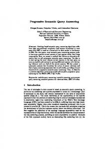
5 Experiments In this section we present a set of experiments evaluating the techniques described above. In appendix we ran additional controlled experiments using an OBDA benchmark built on top of the Wisconsin benchmark [8], and obtain similar results to the ones here. Statoil Scenario In this section we briefly describe the Statoil use-case, and the challenges it presents for OBDA. At Statoil, users access several databases on a daily basis, and one of the most important ones is the Exploration and Production Data Store (EPDS) database. EPDS is a large legacy SQL (Oracle 10g) database comprising over 1500 tables (some of them with up to 10 million tuples) and 1600 views. The complexity of the SQL schema of EPDS is such that it is counter-productive and error-prone to manually write queries over the relational database. Thus, end-users either use only a set of tools with predefined SQL queries to access the database, or interact with IT experts so as to formulate the right query. The latter process can take weeks. This situation triggered the introduction of OBDA in Statoil in the context of the Optique project [13]. In order to test OBDA at Statoil, the users provided 60 queries (in natural language) that are relevant to their job, and that cannot be easily performed or formulated at the moment. The Optique partners formulated these queries in SPARQL, and handcrafted an ontology, and a set of mappings connecting EPDS to the ontology. The ontology contains 90 classes, 37 object properties, and 31 data properties; and there are more than 140 mappings. The queries have between 0 to 2 complex filter expressions (with several arithmetic and string operations), 0 to 5 nested optionals, modifiers such as ORDER BY and DISTINCT, and up to 32 joins. Experiment Results. The queries were executed sequentially on a HP ProLiant server with 24 Intel Xeon CPUs (X5650 @ 2.67 GHz), 283 GB of RAM. Each query was evaluated three times and we took the average. We ran the experiments with 4 exact concepts and 15 virtual functional dependencies, found with our tools and validated by database experts. The 60 SPARQL queries have been executed over Ontop with and without the optimizations for exact predicates and virtual functional dependencies. We consider that a query times out if the average execution time is greater than 20 minutes. The results are summarized in Table 1 and Figure 1. We can see that the proposed optimizations allow Ontop to critically reduce the query size and improve the performance of the query execution by orders of magnitude. Specifically, in Figure 1 we compare standard optimizations with and without the techniques presented here. Observe

Query execution time

14

Dag Hovland1 , Davide Lanti2 , Martin Rezk2 , and Guohui Xiao2 20 m 10 s 4 0.1 s ·10

standard optimizations

standard optimizations + VFD + exact predicates

Fig. 1: Comparison of query execution time with standard optimizations.Log. scale that the average successful query execution time is higher with new optimizations than without because the number of successfully executed queries increases. With standard optimizations, 17 SPARQL queries time out. With both novel optimizations enabled, only four queries still time out. A total of 27 SPARQL queries get a more compact SQL translation with new optimizations enabled. The largest proportional decrease in size of the SQL query is 94%, from 171k chars, to 10k. The largest absolute decrease in size of the SQL is 408k chars. Note that the number of unions in the SQL may decrease also only with VFD-based optimization. Since the VFD-based optimization removes joins, more unions may become equivalent and are therefore removed. The maximum measured decrease in execution time is on a query that times out with standard optimizations, but uses 3.7 seconds with new optimizations.

6 Related work Dependencies have been intensively studied in the context of traditional relational databases [3]. Our work is related to the one in [24]; in particular their notion of path functional dependency is close to the notion of path VFD presented here. However, they do not consider neither ontologies, nor databases, and their dependencies are not meant to be used to optimize queries. There are a number of studies on functional dependencies in RDF [25,12], but as shown in Example 12, functional dependencies in RDF do not necessarily correspond to a VFD (when considering the ontology). Besides, these works do not tackle the issue of SQL query optimization. The notion of perfect mapping [9] is strongly related to the notion of exact mapping. However there is a substantial difference: a perfect mapping must be entailed by the OBDA specification, whereas exact mappings are additional constraints that enrich the OBDA specification. For instance, perfect mappings would not be effective in the Statoil use case, where organizational constraints and storage policies are not entailed by the OBDA specification. The notion of EBox [22,18] was proposed as an attempt to include constraints in OBDA. However, EBox axioms are defined through a T -box like syntax. These axioms cannot express constraints based on templates like virtual functional dependencies.

7 Conclusions In this work we presented two novel optimization techniques for OBDA that complement standard optimizations in the area, and enable efficient SPARQL query answering over enterprise relational data. We provided theoretical foundations for these techniques


15

based on two novel OBDA constraints: virtual functional dependencies, and exact predicates. We implemented these techniques in our OBDA system Ontop and empirically showed their effectiveness through extensive experiments that display improvements on the query execution time up to orders of magnitude. Acknowledgement. This work is partially supported by the EU under IP project Optique (Scalable End-user Access to Big Data), grant agreement n. FP7-318338.

References 1. S. Abiteboul, R. Hull, and V. Vianu. Foundations of Databases. Addison Wesley Publ. Co., 1995. 2. F. Baader, D. Calvanese, D. McGuinness, D. Nardi, and P. F. Patel-Schneider, editors. The Description Logic Handbook: Theory, Implementation and Applications. Cambridge University Press, 2nd edition, 2007. 3. C. Beeri and M. Y. Vardi. The implication problem for data dependencies. In Proc. of ICALP, volume 115 of LNCS, pages 73–85. Springer, 1981. 4. M. Bienvenu, M. Ortiz, M. Simkus, and G. Xiao. Tractable queries for lightweight description logics. In Proc. of IJCAI. IJCAI/AAAI, 2013. 5. D. Calvanese, G. De Giacomo, D. Lembo, M. Lenzerini, and R. Rosati. Tractable reasoning and efficient query answering in description logics: The DL-Lite family. JAR, 39(3):385–429, 2007. 6. U. S. Chakravarthy, D. H. Fishman, and J. Minker. Semantic query optimization in expert systems and database systems. In Proc. of DEXA, pages 659–674, 1986. 7. S. Das, S. Sundara, and R. Cyganiak. R2RML: RDB to RDF mapping language. W3C Recommendation, W3C, Sept. 2012. Available at http://www.w3.org/TR/r2rml/. 8. D. J. DeWitt. The wisconsin benchmark: Past, present, and future. In J. Gray, editor, The Benchmark Handbook. Morgan Kaufmann, 1993. 9. F. Di Pinto, D. Lembo, M. Lenzerini, R. Mancini, A. Poggi, R. Rosati, M. Ruzzi, and D. F. Savo. Optimizing query rewriting in ontology-based data access. In Proc. of EDBT, pages 561–572. ACM Press, 2013. 10. B. Glimm and C. Ogbuji. SPARQL 1.1 entailment regimes. W3C Recommendation, W3C, Mar. 2013. Available at http://www.w3.org/TR/sparql11-entailment/. 11. G. Gottlob, S. Kikot, R. Kontchakov, V. V. Podolskii, T. Schwentick, and M. Zakharyaschev. The price of query rewriting in ontology-based data access. AIJ, 213:42–59, 2014. 12. B. He, L. Zou, and D. Zhao. Using conditional functional dependency to discover abnormal data in RDF graphs. In Proc. of SWIM, pages 43:1–43:7. ACM, 2014. 13. D. Hovland, D. Lanti, M. Rezk, and G. Xiao. OBDA constraints for effective query answering (extended version). http://www.inf.unibz.it/˜ dlanti/pdf/tr-constraints.pdf , 2016. 14. S. Kikot, R. Kontchakov, V. V. Podolskii, and M. Zakharyaschev. Exponential lower bounds and separation for query rewriting. In Proc. of ICALP, pages 263–274. Springer, 2012. 15. S. Kikot, R. Kontchakov, and M. Zakharyaschev. Conjunctive query answering with OWL 2 QL. In Proc. of KR, pages 275–285, 2012. 16. R. Kontchakov, M. Rezk, M. Rodriguez-Muro, G. Xiao, and M. Zakharyaschev. Answering SPARQL queries over databases under OWL 2 QL entailment regime. In Proc. of ISWC, volume 8796 of LNCS, pages 552–567. Springer, 2014. 17. D. Lanti, M. Rezk, G. Xiao, and D. Calvanese. The NPD benchmark: Reality check for OBDA systems. In Proc. of EDBT, 2015. 18. J. Mora, R. Rosati, and O. Corcho. kyrie2: Query rewriting under extensional constraints in elhio. In Proc. of ISWC, pages 568–583, 2014.

16


19. A. Poggi, D. Lembo, D. Calvanese, G. De Giacomo, M. Lenzerini, and R. Rosati. Linking data to ontologies. J. on Data Semantics, X:133–173, 2008. 20. M. Rodriguez-Muro, R. Kontchakov, and M. Zakharyaschev. Ontology-based data access: Ontop of databases. In Proc. of ISWC, volume 8218 of LNCS, pages 558–573. Springer, 2013. 21. M. Rodriguez-Muro and M. Rezk. Efficient SPARQL-to-SQL with R2RML mappings. J. of Web Semantics, 2015. 22. R. Rosati. Prexto: Query rewriting under extensional constraints in DL-Lite. In Proc. of ESWC, pages 360–374, 2012. 23. R. Rosati and A. Almatelli. Improving query answering over DL-Lite ontologies. In Proc. of KR, pages 290–300, 2010. 24. G. E. Weddell. Reasoning about functional dependencies generalized for semantic data models. ACM Trans. Database Syst., 17(1):32–64, Mar. 1992. 25. Y. Yu and J. Heflin. Extending functional dependency to detect abnormal data in RDF graphs. In Proc. of ISWC, volume 7031, pages 794–809. Springer, October 2011.


A

17

Appendix

A.1 Background On SPARQL to SQL In this section, we recap the complete SPARQL to SQL translation [16]. This background will be used for the proofs in the following sections. SPARQL under Simple Entailment SPARQL is a W3C standard language designed to query RDF graphs. Its vocabulary contains four pairwise disjoint and countably infinite sets of symbols: I for IRIs, B for blank nodes, L for RDF literals, and V for variables. The elements of C = I ∪ B ∪ L are called RDF terms. A triple pattern is an element of (C ∪ V) × (I ∪ V) × (C ∪ V). A basic graph pattern (BGP) is a finite set of triple patterns. Finally, a graph pattern, P, is an expression defined by the grammar P ::= BGP | Filter(P, F) | Bind(P, v, c) | Union(P1 , P2 ) | Join(P1 , P2 ) | Opt(P1 , P2 , F), where F, a filter, is a formula constructed from atoms of the form bound(v), (v = c), (v = v′ ), for v, v′ ∈ V, c ∈ C, and possibly other built-in predicates using the logical connectives ∧ and ¬. The set of variables in P is denoted by var(P). A SPARQL query is a graph pattern P with a solution modifier, which specifies the answer variables—the variables in P whose values we are interested in—and the form of the output (we ignore other solution modifiers for simplicity). The values to variables are given by solution mappings, which are partial maps s : V → C with (possibly empty) domain dom(s). In this paper, we use the set-based (rather than bag-based, as in the specification) semantics for SPARQL. For sets S 1 and S 2 of solution mappings, a filter F, a variable v ∈ V and a term c ∈ C, let – – – – –

Filter(S , F) = {s ∈ S | F s = ⊤}; Bind(S , v, c) = {s ⊕ {v 7→ c} | s ∈ S } (provided that v < dom(s), for s ∈ S ); Union(S 1 , S 2 ) = {s | s ∈ S 1 or s ∈ S 2 }; Join(S 1 , S 2 ) = {s1 ⊕ s2 | s1 ∈ S 1 and s2 ∈ S 2 are compatible}; Opt(S 1 , S 2 , F) = Filter(Join(S 1 , S 2 ), F) ∪ {s1 ∈ S 1 | for all s2 ∈ S 2 , either s1 , s2 are incompatible or F s1 ⊕s2 , ⊤}.

Here, s1 and s2 are compatible if s1 (v) = s2 (v), for any v ∈ dom(s1 ) ∩ dom(s2 ), in which case s1 ⊕ s2 is a solution mapping with s1 ⊕ s2 : v 7→ s1 (v), for v ∈ dom(s1 ), s1 ⊕ s2 : v 7→ s2 (v), for v ∈ dom(s2 ), and domain dom(s1 ) ∪ dom(s2 ). The truth-value F s ∈ {⊤, ⊥, ε} of a filter F under a solution mapping s is defined inductively: – (bound(v)) s is ⊤ if v ∈ dom(s) and ⊥ otherwise; – (v = c) s = ε if v < dom(s); otherwise, (v = c) s is the classical truth-value of the predicate s(v) = c; similarly, (v = v′ ) s = ε if either v or v′ < dom(s); otherwise, ′ (v = v′ ) s is the classical truth-value of the predicate  s(v) = s(v ); s  (  ⊥, if F1 = ⊥ or F2s = ⊥,   ε, if F s = ε,  s s – (¬F) = and (F1 ∧ F2 ) =  ⊤, if F1s = F2s = ⊤,   ¬F s , otherwise,  ε, otherwise.

18


Finally, given an RDF graph G, the answer to a graph pattern P over G is the set ~PG of solution mappings defined by induction using the operations above and starting from the following base case: for a basic graph pattern B, ~BG = {s : var(B) → C | s(B) ⊆ G},

(2)

where s(B) is the set of triples resulting from substituting each variable u in B by s(u). This semantics is known as simple entailment. Translating SPARQL under Simple Entailment to SQL We recap the basics of relational algebra and SQL (see e.g., [1]). Let U be a finite (possibly empty) set of attributes. A tuple over U is a map t : U → ∆, where ∆ is the underlying domain, which always contains a distinguished element null. A (|U|-ary) relation over U is a finite set of tuples over U (again, we use the set-based rather than bag-based semantics). A filter F over U is a formula constructed from atoms isNull(U ′ ), (u = c) and (u = u′ ), where U ′ ⊆ U, u, u′ ∈ U and c ∈ ∆, using the connectives ∧ and ¬. Let F be a filter with variables U and let t be a tuple over U. The truth-value F t ∈ {⊤, ⊥, ε} of F over t is defined inductively: – (isNull(U ′ ))t is ⊤ if t(u) is null, for all u ∈ U ′ , and ⊥ otherwise; – (u = c)t = ε if t(u) is null; otherwise, (u = c)t is the classical truth-value of the predicate t(u) = c; similarly, (u = u′ )t = ε if either t(u) or t(u′ ) is null; otherwise, ′ (u = u′ )t is the classical truth-value of the predicate  t(u) = t(u );  t t     ε, ⊥, if F1t = ⊥t or F2 = ⊥, if F t = ε,   t t – (¬F) =  and (F1 ∧ F2 ) =  ⊤, if F1 = F2 = ⊤,   ¬F t , otherwise,   ε, otherwise.

(Note that ¬ and ∧ are interpreted in the same three-valued logic as in SPARQL.) We use standard relational algebra operations such as union, difference, projection, selection, renaming and natural (inner) join. Let Ri be a relation over Ui , i = 1, 2.

If U1 = U2 then the standard R1 ∪ R2 and R1 \ R2 are relations over U1 . If U ⊆ U1 then πU R1 = R1 |U is a relation over U. If F is a filter over U1 then σF R1 = {t ∈ R1 | F t = ⊤} is a relation over U1 . If v < U1 and u ∈ U1 then ρv/u R1 = tv/u | t ∈ R1 , where tv/u : v 7→ t(u) and ′ ′ ′ tv/u : u 7→ t(u ), for u ∈ U1 \ {u}, is a relation over (U1 \ {u}) ∪ {v}. – R1 Z R2 = {t1 ⊕ t2 | t1 ∈ R1 and t2 ∈ R2 are compatible} is a relation over U1 ∪ U2 . Here, t1 and t2 are compatible if t1 (u) = t2 (u) , null, for all u ∈ U1 ∩ U2 , in which case a tuple t1 ⊕ t2 over U1 ∪ U2 is defined by taking t1 ⊕ t2 : u 7→ t1 (u), for u ∈ U1 , and t1 ⊕ t2 : u 7→ t2 (u), for u ∈ U2 (note that if u is null in either of the tuples then they are incompatible).

– – – –

To bridge the gap between partial functions (solution mappings) in SPARQL and total mappings (on attributes) in SQL, we require one more operation (expressible in SQL): – If U ∩ U1 = ∅ then the padding µU R1 is R1 Z nullU , where nullU is the relation consisting of a single tuple t over U with t : u 7→ null, for all u ∈ U.


19

By an SQL query, Q, we understand any expression constructed from relation symbols (each over a fixed set of attributes) and filters using the relational algebra operations given above (and complying with all restrictions on the structure). Suppose Q is an SQL query and D a data instance which, for any relation symbol in the schema under consideration, gives a concrete relation over the corresponding set of attributes. The answer to Q over D is a relation kQkD defined inductively in the obvious way starting from the base case: for a relation symbol Q, kQkD is the corresponding relation in D. We now define a translation, τ, which, given a graph pattern P, returns an SQL query τ(P) with the same answers as P. More formally, for a set of variables V, let extV be a function transforming any solution mapping s with dom(s) ⊆ V to a tuple over V by padding it with nulls: extV (s) = {v 7→ s(v) | v ∈ dom(s)} ∪ {v 7→ null | v ∈ V \ dom(s)}. The relational answer to P over G is kPkG = {extvar(P) (s) | s ∈ ~PG }. The SQL query τ(P) will be such that, for any RDF graph G, the relational answer to P over G coincides with the answer to τ(P) over triple(G), the database instance storing G as a ternary relation triple with the attributes subj, pred, obj. First, we define the translation of a SPARQL filter F by taking τ(F) to be the SQL filter obtained by replacing each bound(v) with ¬isNull(v) (other built-in predicates can be handled similarly). Proposition 2. Let F be a SPARQL filter and let V be the set of variables in F. Then F s = (τ(F))extV (s) , for any solution mapping s with dom(s) ⊆ V. The definition of τ proceeds by induction on the construction of P. Note that we can always assume that graph patterns under simple entailment do not contain blank nodes because they can be replaced by fresh variables. It follows that a BGP {tp1 , . . . , tpn } is equivalent to Join({tp1 }, Join({tp2 }, . . . )). So, for the basis of induction we set   π∅ σ(subj=s)∧(pred=p)∧(obj=o) triple, if s, p, o ∈ I ∪ L,         π s ρ s/subj σ(pred=p)∧(obj=o) triple, if s ∈ V and p, o ∈ I ∪ L,  τ({hs, p, oi}) =  π s,oρ s/subj ρo/obj σpred=p triple, if s, o ∈ V, s , o, p ∈ I ∪ L,       π ρ σ triple, if s, o ∈ V, s = o, p ∈ I ∪ L, s s/subj (pred=p)∧(subj=obj)    . . .

(the remaining cases are similar). Now, if P1 and P2 are graph patterns and F1 and F are filters containing only variables in var(P1 ) and var(P1 ) ∪ var(P2 ), respectively, then we set Ui = var(Pi ), i = 1, 2, and τ(Filter(P1 , F1 )) = στ(F1 ) τ(P1 ), τ(Bind(P1 , v, c)) = τ(P1 ) Z {v 7→ c}, τ(Union(P1 , P2 )) = µU2 \U1 τ(P1 ) ∪ µU1 \U2 τ(P2 ), [ (πU1 \V1 σisNull(V1 ) τ(P1 )) Z (πU2 \V2 σisNull(V2 ) τ(P2 )) , τ(Join(P1 , P2 )) = V1 ,V2 ⊆U1 ∩U2 V1 ∩V2 =∅

τ(Opt(P1 , P2 , F)) = τ(Filter(Join(P1 , P2 ), F)) ∪ [ µV1 πU1 \V1 τ(Filter(Join(PV1 1 ,U1 ∩U2 , P2 ), F)) , µU2 \U1 τ(P1 ) \ V1 ⊆U1 ∩U2

20


V V where PV,U = Filter(P, v∈V ¬bound(v) ∧ v∈U\V bound(v)). It is readily seen that any τ(P) is a valid SQL query and defines a relation over var(P); in particular, τ(Join(P1 , P2 )) S is a relation over i=1,2 (Ui \ Vi ) = U1 ∪ U2 = var(Join(P1 , P2 )). Theorem 2. For any RDF graph G and any graph pattern P, kPkG = kτ(P)ktriple(G) .

R2RML Mappings The SQL translation of a SPARQL query constructed above has to be evaluated over the ternary relation triple(G) representing the virtual RDF graph G. Our aim now is to transform it to an SQL query over the actual database, which is related to G by means of an R2RML mapping [7]. We begin with a simple example. Example 17. The following R2RML mapping (in the Turtle syntax) populates an object property ub:UGDegreeFrom from a relational table students, whose attributes id and degreeuniid identify graduate students and their universities: :m1 a rr:TripleMap; rr:logicalTable [ rr:sqlQuery ”SELECT * FROM students WHERE stype=1” ]; rr:subjectMap [ rr:template ”/GradStudent{id}” ] ; rr:predicateObjectMap [ rr:predicate ub:UGDegreeFrom ; rr:objectMap [ rr:template ”/Uni{degreeuniid}” ] ]

More specifically, for each tuple in the query, an R2RML processor generates an RDF triple with the predicate ub:UGDegreeFrom and the subject and object constructed from attributes id and degreeuniid, respectively, using IRI templates. Our aim now is as follows: given an R2RML mapping M, we are going to define an SQL query trM (triple) that constructs the relational representation triple(G D,M ) of the virtual RDF graph G D,M obtained by M from any given data instance D. Without loss of generality and to simplify presentation, we assume that each triple map has – one logical table (rr:sqlQuery), – one subject map (rr:subjectMap), which does not have resource typing (rr:class), – and one predicate-object map with one rr:predicateMap and one rr:objectMap. This normal form can be achieved by introducing predicate-object maps with rdf:type and splitting any triple map into a number of triple maps with the same logical table and subject. We also assume that triple maps contain no referencing object maps (rr:parentTriplesMap, etc.) since they can be eliminated using joint SQL queries [7]. Finally, we assume that the term maps (i.e., subject, predicate and object maps) contain no constant shortcuts and are of the form [rr:column v], [rr:constant c] or [rr:template s]. Given a triple map m with a logical table (SQL query) R, we construct a selection σ¬isNull(v1 ) · · · σ¬isNull(vk ) R, where v1 , . . . , vk are the referenced columns of m (attributes of R in the term maps in m)—this is done to exclude tuples that contain null [7]. To construct trm , the selection filter is prefixed with projection πsubj,pred,obj and, for each of the three term maps, either with renaming (e.g., with ρobj/v if the object map is of the form [rr:column v]) or with value creation (if the term map is of the form [rr:constant c] or [rr:template s]; in the latter case, we use the built-in string concatenation function ). For instance, the mapping :m1 from Example 17 is converted to the SQL query SELECT (’/GradStudent’ id) AS subj, ’ub:UGDegreeFrom’ AS pred, (’/Uni’ degreeuniid) AS obj FROM students WHERE (id IS NOT NULL) AND (degreeuniid IS NOT NULL) AND (stype=1).


Given an R2RML mapping M, we set trM (triple) =

S

m∈M

21

trm .

Proposition 3. For any R2RML mapping M and data instance D, t ∈ ktrM (triple)kD if and only if t ∈ triple(G D,M ). Finally, given a graph pattern P and an R2RML mapping M, we define trM (τ(P)) to be the result of replacing every occurrence of the relation triple in the query τ(P), constructed in Section A.1, with trM (triple). By Theorem 2 and Proposition 3, we obtain: Theorem 3. For any graph pattern P, R2RML mapping M and data instance D, kPkGD,M = ktrM (τ(P))kD . A.2 Proofs of Section 4.1 Proposition 1. Let M′ be exact for the predicate A in T . Let M′T be the result of ′ replacing all the mappings defining A in MT by M′ . Then GO = G((∅,MT ,Σ),D) . Proof (Sketch). By the definition of T -mappings, we have GO = G∅,MT ,D . For all predicates other than A, MT and M′T produce the same set of triples since the mappings defining them are identical. For the predicate A, since M′ is exact in O, MT and M′T ′ also produce same set of triples. Therefore G∅,MT ,D = G∅,MT ,D . A.3 Proofs of Section 4.2 Lemma 1. Let P1 , . . . , Pn be properties in T such that, for each 1 ≤ i < n, tdi = td1 . Then, the VFD td1 7→b P1 . . . Pn is satisfied in O if and only if, for each 1 ≤ i ≤ n, the FD xi → yi is satisfied on sqli (zi )D . Proof. td1 7→b P1 . . . Pn is satisfied in GO m (Definition 3) O O ∀s ∈ S t1 : ∀1 ≤ i ≤ n : (s, o) ∈ PGi ∧ (s, o′ ) ∈ PGi ⇒ o = o′ d m (Mappings assumptions for Pi ) ∀1 ≤ i ≤ n : ∀u ∈ πxi σnotNull(xi ,yi ) sqli (zi )D : (u, y) ∈ πxi yi σnotNull(xi ,yi ) sqli (zi )D ∧ (u, y’) ∈ πxi yi σnotNull(xi ,yi ) sqli (zi )D ⇒ y = y’ m (Definition of Functional Dependency) ∀1 ≤ i ≤ n : xi → yi is satisfied in πxi yi σnotNull(xi ,yi ) sqli (zi )D m ∀1 ≤ i ≤ n : xi → yi is satisfied in σnotNull(xi ,yi ) sqli (zi )D

Lemma 2. Consider n properties P1 , . . . , Pn in T with for which td1 b P1 · · · Pn is satisfied in O. Then

tdi

=

td1 ,

for each 1 ≤ i ≤ n, and

πγ (sql1 (z1 ))D = πγ (sql1 (z1 ) Zx1 =x2 sql2 (z2 ) Z · · · Zx1 =xn sqln (zn ))D ,

where γ = x1 , y1 , . . . , yn .


22

Proof. The direction ⊆ of the equality can be obtained easily. Here we prove the direction ⊇. D Let qbranch denote the right hand side expression in the equality. Assume the containment ⊇ does not hold. Then, this means there exists a tuple (s, v1 , . . . , vn ) such that D – (u, v1 , . . . , vn ) ∈ qbranch , and – (u, v1 , . . . , vn ) < πx1 ,v1 ,...,vn σnotNull(x1 ,y1 ) sql1 (z1 )D

The above implies that there exists an index j, 1 ≤ j ≤ n, such that D – (u, v j ) ∈ πx1 ,y j qbranch , and – (u, v j ) < πx1 ,y j σnotNull(x1 ,y1 ) sql1 (z1 )D

Then, we can distinguish three cases: 1. u < πx1 σnotNull(x1 ,y1 ) sql1 (z1 ). D D Then u < πx1 qbranch , hence (u, v j ) < πx1 ,y j qbranch ; contradiction. ′ ′ 2. (u, v j ) ∈ πx1 ,y j σnotNull(x1 ,y1 ) sql1 (z1 ), and v j = null. Since td1 b P1 · · · Pn is satisfied in O, it must be (u, null) ∈ πx j ,y j σnotNull(x j ,y j ) sql j (z j )D , which is impossible. 3. (u, v′j ) ∈ πx1 ,y j σnotNull(x1 ,y1 ) sql1 (z1 )D , v j , v′j and not v j nor v′j is null. b P1 · · · Pn is satisfied in O, because of This violates the hypothesis that td1 Lemma 1. Hence, by contradiction we conclude that the containment ⊇ must hold. Results and Proofs for PATH VFDs Lemma 3. Let P1 , . . . , Pn be properties in T such that, for each 1 ≤ i ≤ n, tri = tdi+1 . Then, the VFD td1 7→ p P1 . . . Pn is satisfied in O if and only if the FD x1 → y1 · · · yn is satisfied in: πx1 y1 ···yn (sql1 (z1 )) Zy1 =x2 sql2 (z2 ) Zy2 =x3 · · · Zyn−1 =xn sqln (zn ))D Proof. td1 7→ p P1 . . . Pn is satisfied in GO m (Definition 3) ∀s ∈ S 1td : ∃ unique list ho1 , . . . , on i in GO such that {(s, P1 , o1 ), . . . , (on−1 , Pn , on )} ⊆ GO m O O V O O ∀s ∈ S 1td : ∀o1 , . . . , on , o′1 , . . . , o′n in GO : (s, o1 ) ∈ PG1 ∧ . . . ∧ (on−1 , on ) ∈ PGn (s, o′1 ) ∈ PG1 ∧ . . . ∧ (o′n−1 , o′n ) ∈ PGn ⇒ ′ ′ o1 = o1 , . . . , on = on m (Mappings assumptions for Pi ) ∀u ∈ πx1 σnotNull(x1 ) sql1 (z1 )D : ∀v1 , v′1 ∈ πy1 σnotNull(y1 ) sql1 (z1 )D : . . . : ∀vn , v′n ∈ πyn σnotNull(yn ) sqln (zn )D : (u, v1 ) ∈ πx1 y1 σnotNull(x1 ,y1 ) sql1 (z1 )D ∧ . . . ∧ (vn−1 , vn ) ∈ πxn yn σnotNull(xn ,yn ) sqln (zn )D

^

(u, v′1 ) ∈ πx1 y1 σnotNull(x1 ,y1 ) sql1 (z1 )D ∧ . . . ∧ (v′n−1 , v′n ) ∈ πxn yn σnotNull(xn ,yn ) sqln (zn )D ⇒ v1 = v′1 , . . . , vn = v′n


23

m (Standard Translation AND assumptions on templates)

∀u ∈ πx1 σnotNull(x1 ) sql1 (z1 )D : ∀v1 , v′1 ∈ πy1 σnotNull(y1 ) sql1 (z1 )D : . . . : ∀vn , v′n ∈ πyn σnotNull(yn ) sqln (zn )D : D [ (u, v1 , . . . , vn ) ∈ πx1 y1 ...yn (σnotNull(x1 ,y1 ) sql 1 (z1 ) Zy1 =x2 σnotNull(x2 ,y2 ) sql2 (z2 ) Zy2 =x3 · · · Zyn−1 =xn σnotNull(xn ,yn ) sqln (zn ))

^

D [ (u, v′1 , . . . , v′n ) ∈ πx1 y1 ...yn (σnotNull(x1 ,y1 ) sql 1 (z1 ) Zy1 =x2 σnotNull(x2 ,y2 ) sql2 (z2 ) Zy2 =x3 · · · Zyn−1 =xn σnotNull(xn ,yn ) sqln (zn )) ⇒

v1 = v′1 , . . . , vn = v′n

m (Definition of Functional Dependency) D [ x1 → y1 . . . yn is satisfied in πx1 y1 ...yn ( sql 1 (z1 ) Zy1 =x2 sql2 (z2 ) Zy2 =x3 · · · Zyn−1 =xn sqln (zn ))

Example 18. Consider the following set of T -mappings for an OBDA setting O: f(id,name) P1 g(friend) ← SELECT id, name, friend FROM T g(friend) P2 h(friend age) ← SELECT friend, friend age FROM T

Then the lemma above suggests that the VFD f 7→ p P1 P2 is satisfied in O if and only if the FD id name → friend friend age is satisfied in (T Z f riend= f riend T )D . Definition 9 (Optimizing Path VFD). Let t be a template, and P1 , . . . , Pn be properp ties in T . An optimizing path VFD is an expression of the form t P1 · · · Pn . An p p optimizing VFD t P1 · · · Pn is satisfied in O if t 7→ P1 · · · Pn is satisfied in O and πx1 y1 ...yn sql1 (z1 )D ⊆ qDpath

(3)

where q path = πx1 y1 ...yn (sql1 (z1 ) Zy1 =x2 sql2 (z2 ) Zy2 =x3 · · · Zyn−1 =xn sqln (zn )). Lemma 4. Consider n properties P1 , . . . , Pn in T with tri = tdi+1 , for each 1 ≤ i < n, and for which td1 p P1 · · · Pn is satisfied in O. Then πx1 y1 ...yn sql1 (z1 )D = qDpath where q path is the same as in the Definition 9. Proof. (Sketch) The argument is similar to the one of the proof for Lemma 2, by using Lemma 3. p Definition 10 (Optimizable path BGP). A BGP β is optimizable w.r.t. v = td P1 . . . Pn if (i) v is satisfied in O; (ii) the BGP of triple patterns in β involving properties is of the form ?v0 P1 ?v1 . ...?vn−1 Pn ?vn .; and (iii) for every triple pattern of the d form ?u rdf:type C in β, ?u is the subject of some Pi (i = 1 . . . n) and tdi Pi C is i r satisfied in O , or ?u is the object of some Pi (i = 1 . . . n) and tr Pi C is satisfied in O.

24


Proofs for Main Results x Theorem 1. Let β be an optimizable BGP w.r.t. td P1 . . . Pn (x = b, p) in O. Let πv/td1 ,v1 /tr1 ,...,vn /trn sqlβ be the SQL translation of β as explained in Section 3. Let sql′β = sql1 (x1 , y1 . . . , yn ). Then sqlβD and sql′D β return the same answers. p

Proof. Assume that td P1 ...Pn . The proof for branching functional dependencies is analogous. From the definition of τ for triple pattern and the definition of the τ for Z for BGPs it follows that the BGP β will be translated as: (πv0,v1 ρv/subj ρv1 /obj σpred=P1 triple) Zv1 =v2 .. .

(4)

Zvn−2 =vn−1 (πvn−1 ,vn ρvn−1 /subj ρvn /obj σpred=Pn triple) The table triple is replaced by the definition of the triple patterns in the mappings as follows: (πv0,v1 ρv0 /subj ρv1 /obj σpred=P1 πpred/P1 ,subj/td1 ,obj/tr1 (sql1 (z1 ))) Zv1 =v2 .. .

(5)

Zvn−2 =vn−1 (πvn−1 ,vn ρvn−1 /subj ρvn /obj σpred=Pn πpred/Pn ,subj/tdn ,obj/trn )(sqln (zn )))) This expression can be simplified to: (πv0 ,v1 ρv0 /subj ρv1 /obj πsubj/td1 ,obj/tr1 (sql1 (z1 ))) Zv1 =v2 .. .

(6)

Zvn−2 =vn−1 (πvn−1 ,vn ρvn−1 /subj ρvn /obj πsubj/tdn ,obj/trn )(sqln (zn )))) By definition we know that the template in the range of Pi−1 coincide with the template in Pi . Thus, we can remove them from the join over ui ’s in (??) and make the join over the attributes xi , yi instead of the URIs. Therefore, β can be rewritten to πv0 /td1 ,v1 /tr1 ,...,vn /trn (sql1 (z1 ) Zy1 =x2 sql2 (z2 ) Zy2 =x3 · · · Zyn−1 =xn sqln (zn ))

(7)

Since β is optimizable, we know that πx1 y1 ...yn sql1 (z1 ) = πx1 y1 ...yn (sql1 (z1 ) Zy1 =x2 sql2 (z2 ) Zy2 =x3 · · · Zyn−1 =xn sqln (zn ))

(8)

Therefore, we can simplify (7) to πv/td1 ,v1 /tr1 ,...,vn /trn (sql1 (z1 )). This proves the Theorem.


25

A.4 Lifting Basic OBDA Instance Assumption We show that the “basic OBDA instance assumption” in Section 4.2 is not a real restriction. A SPARQL query over a T -mapping with predicates of multiple templates can be rewritten to another SPARQL query over another T -mapping with predicates of only single template. As usual, we assume an OBDA instance ((T , M, Σ), D), and let MT be a T -mapping. Suppose a predicate A is defined by k mapping assertions using different template in MT : A(td1 (x), tr1 (y)) ← sql1 (z) ... A(tdk (x), trk (y)) ← sqlk (z) Define MTA be the mapping obtained by replacing the assertions for the A with the following k mapping assertions defining k fresh predicates Ai (i = 1, . . . , k): A1 (td1 (x), tr1 k(y)) ← sql1 (z) ... Ak (tdk (x), trk (y)) ← sqlk (z) Suppose that Q is a SPARQL query using predicate A. The idea is to construct another SPARQL query Q′ such that ~Q(MT ,D) = ~Q′ (MTA ,D) . The construction is performed on each triple pattern using A. Suppose B is a triple pattern occurring in Q; we take B+ to be the union of B[A 7→ Ai ], i = 1...k where B[A 7→ Ai ] is a triple pattern obtained by replacing all the occurrences of A in B with Ai . Finally Q′ is defined as the SPARQL query obtained by replacing all the triple patterns B with B+. Lemma 5. ~B(MT ,D) = ~B+ (MTA ,D) Proof. We only prove the case where B is a single triple pattern of the form B = (?x, rdf:type, A), since the case where A is a property can be proved analogously. In this case, B+ = (?x, rdf:type, A1 ) Union . . . Union (?x, rdf:type, Ak ) Suppose that {?x 7→ a} is a solution mapping, i.e., A(a) is in the RDF graph exposed by MT and D. It follows that there is a mapping assertion A(t(x)) ← sqli (z) ∈ MT , such that a = t(x0 ) for some template t0 and tuple x0 . Since Ai (t(x)) ← sqli (z) ∈ MTA , we have Ai (t(x0 )) is in the RDF graph exposed by MTA and D. Then {x 7→ a} is a solution mapping of (?x, rdf:type, Ai ) and also of B+ . The other direction can be proved analogously. Theorem 4. ~Q(MT ,D) = ~Q′ (MTA ,D) Proof. The proof is a standard induction over the structure of the SPARQL queries. The base case of proof is the triple pattern case, and has been proved in Lemma 5. The inductive case can be proved easily. By exhaustingly apply Theorem 4 to all predicates of different templates, one can lift the restriction of “basic OBDA instance”.

26


A.5 Wisconsin Benchmark We setup an environment based on the Wisconsin Benchmark [8]. This benchmark was designed for the systematic evaluation of database performance with respect to different query characteristics. The benchmark comes with a schema that is designed so one can quickly understand the structure of each table and the distribution of each attribute value. This allows easy construction of queries that isolate the features that need to be tested. The benchmark also comes with a data generator to populate the schema. Unlike EPDS, the benchmark database contains synthetic data that allows easily specifying a wide range of retrieval queries. For instance, in EPDS it is very difficult to specify a selection query with a 20% or 30% selectivity factor. This task becomes even harder when we include joins into the picture. The benchmark defines a single table schema (which can be used to instantiate multiple tables). The table, which we now call “Wisconsin table”, contains 16 attributes, and a primary key (unique2) with integers from 0 to 100 million randomly ordered. We refer the reader to [8] for details on the algorithm that populates the schema. Dataset We used Postgres 9.1, and DB2 9.7 as Ontop backends. The query optimizers were left with the default configurations. All the table statistics were updated. For each DB engine we created a database, each with 10 tables: 5 Wisconsin tables (Tabi , i = 1, . . . , 5), and 5 tables materializing the join of the former tables. For instance, view123 materializes the join of the tables Tab1, Tab2, and Tab3. Each table contains 100 million rows, and each of the databases occupied ca. 400GB of disk space. Hardware We ran the experiments in an HP Proliant server with 24 Intel Xeon CPUs (@3.47GHz), 106GB of RAM and five 1TB 15K RPM HD. Ontop was run with 6GB Java heap space. The OS is Ubuntu 12.04 LTS 64-bit edition. In these experiments, we ran each query 3 times, and we averaged the execution times. There was a warm-up phase, where we ran 4 random queries not belonging to the tests. Evaluating the Impact of VFD-based Optimization The experiments in this section measure the impact of optimization based on VFDs. Optimizations based on branching VFDs and path VFDs produce the same effect in the resulting SQL query, therefore, for concreteness we focus on branching VFD. The performance gain for path VFD is similar. Recall that we started studying this scenario because EPDS contains thousands of views that lack primary/foreign keys, and some of them cannot be avoided in the mappings. This prevents OBDA semantic optimizations to take place. The following experiments evaluate the trade-off of using views or their definitions depending on: (i) type of mappings (using views or view definitions); (ii) the complexity of the user query (# of SPARQL joins); (iii) the complexity of the mapping definition (# of SQL joins); (iv) the selectivity of the query; (v) the VFD optimization ON/OFF; (vi) the DB engine (DB2/PostgreSQL); In the following we describe the queries, mappings and the OBDA specifications and instances used in the different experiments.


27

Queries In this experiment we tested a set of 36 queries each varying on: (i) the number of SPARQL joins (1-3), (ii) SQL joins in the mappings (1-4), and (iii) selectivity of the query (3 different values). The SPARQL queries have the following shape: SELECT ?x ?y WHERE { ?x a : Class − n − S QLs . ?x : Property1 − n − S QLs ?y1 . . . . ?x : Propertym − n − S QLs ?ym . Filter( ?y m < k% ) }

where Class-n-SQLs and Propertyi-n-SQLs are classes and properties defined by mappings which source is either an SQL join of n = 1 . . . 4 tables, or a materialized view of the join of n tables. Subindex m represents the number of SPARQL joins, 1 to 3. Regarding the selectivity of k%, we did the experiments with the following values: (i) 0.0001% (100 results); (ii) 0.01% (10.000 results); (iii) 0.1% (100.000 results). These queries do not belong to the Wisconsin benchmark. OBDA Specifications We have two OBDA settings, one where classes and properties are populated using an SQL that use original tables with primary keys (1-4 joins) (K1 ); and a second one where predicates are populated using materialized views (materializing 1-4 joins). This second setting we tested with VFD optimization (K2 ) and without optimization (K3 ). In the first OBDA setting, all the property subjects are mapped into the tables primary keys. There are no axioms in the ontology. All the individuals have the same template t. Let S t be the set of all individuals. In K2 there are 12 branching VFDs of the form S t 7→b :Propertym -n-SQLs for every n = 1 . . . 4, m = 1 . . . 3. The optimizable VFDs contain intuitively the properties populated from the same view, that is, S t 7→b :Property1 -n-SQLs, :Property2 -n-SQLs, :Property3 -n-SQLs for n = 1 . . . 4. Discussion and Results The results of the experiments are shown in Figure 2. Each qi/ j represents the query with i SPARQL joins over properties mapped to j SQL joins. There is almost no difference between the results with different selectivity, so for clarity we averaged the run times over different selectivities. Since the experiment was run three times, each point in the figure represents the average of 9 query executions. The experiment results in Figure 2 show that all the SPARQL queries perform better in K2 than in K3 in both DB engines. Moreover, in all cases queries in K2 perform at least twice as fast as the ones in K3 , even getting close to the performance of K1 . In Ontop -Postgres, the execution of the hardest SPARQL queries in K1 is 1 order of magnitude faster than in K2 . The execution of these queries in K2 is 4 times faster than in K3 . In Ontop -DB2, the performance gap between the SPARQL queries in K3 and K2 is smaller. The SPARQL queries in K1 are slightly faster than the queries in K2 . The execution in K2 is 2 times faster than in K3 . In Ontop -Postgres and Ontop -DB2, the translations of the SPARQL queries resulting from the K3 scenario contain self-joins of the non-indexed views that force the DB engines to create hash tables for all intermediate join results which increases the start-up cost of the joins, and the overall execution time. One can observe that in both, Ontop -Postgres and Ontop -DB2, the number of SPARQL joins strongly affect the performance of the query in K3 . In both cases, the SPARQL queries in K2 , because of our

28

Dag Hovland1 , Davide Lanti2 , Martin Rezk2 , and Guohui Xiao2 Postgres 16 m 14 m 12 m 10 m 8m 6m 4m 2m q1/1

q1/2

q1/3

q2/1

q2/2

q2/3

q3/1

q3/2

q3/3

q4/1

q4/2

q4/3

q3/2

q3/3

q4/1

q4/2

q4/3

DB2 16 m 14 m 12 m 10 m 8m 6m 4m 2m q1/1

q1/2

q1/3

q2/1

q2/2

q2/3

q3/1

K1 (Querying the tables directly) K2 (Views with optimization enabled) K3 (Views no optimization)

Fig. 2: Experiments showing the impact of the optimization technique based on VFD optimization technique, get translated into a join-free SQL query that requires a single sequential scan of the unindexed view. However, the cost of scanning the whole view to perform a non-indexed filter is still higher than the cost of joins (nested joins in both) of the indexed tables in K1 . Evaluating the Impact of Exact Mappings In this test we evaluate the exact mapping optimization technique described in Section 4.1. This experiment is inspired by the use case in EPDS where optimization based on exact mapping can help. The following experiments evaluate the impact of the optimization depending on: (i) the complexity of the query (# of SPARQL joins); (ii) the selectivity of the query; (iii) the number of specified exact classes; (iv) the DB engine (DB2/PostgreSQL). In the following we describe the tables, ontology, mappings, queries and exact predicate specifications used in the experiment. OBDA Specifications The ontology contains four classes A1 , A2 , A3 , A4 , one object property R and one data property S . The classes form a hierarchy A1

rdfs:subClassOf

A2 , A2

rdfs:subClassOf A3 ,

A3 rdfs:subClassOf A4 .

The mappings for classes Ai (i = 1, . . . , 4) are defined over the primary key of Tabi with different filters, in such a way that each Ai is exact. The mappings for R and S are defined over the primary key column and another unique column (unique1) of Tab5 . Queries In this experiment we tested 6 queries (q1 , . . . , q6 ) varying on: (i) the number of classes and properties in the SPARQL (1-3) and (ii) the classes used in the query. For instance, q3 is


29

Postgres 20 m 18 m 16 m 14 m 12 m 10 m 8m 6m 4m 2m q1

q2

q3

q4

q5

q6

q5

q6

DB2 20 m 18 m 16 m 14 m 12 m 10 m 8m 6m 4m 2m q1

q2

q3

E0 (No exact mappings) E2 (2 exact mappings)

q4

E1 (1 exact mapping) E2 (3 exact mappings)

Fig. 3: Experiments showing the impact of the optimization technique based on Exact Mappings SELECT * WHERE {?x a :A3. ?x :R y. ?y a :A4. OPTIONAL { ?x :S ?u . } OPTIONAL { ?y :S ?v . }. }

Exact Concepts We consider the following four exact concept specifications: E0 = ∅, E1 = {A1 , A2 }, E2 = {A1 , A2 , A3 }, E3 = {A1 , A2 , A3 , A4 }. Observe that E0 corresponds to the case where no exact mapping optimization is applied. Discussion and Results The results of the experiments are shown in Figure 3. The results show that the exact mapping optimization improves the performance of all SPARQL queries in both database engines. In particular, under the full optimization setting E3 , none of the queries time out (20 mins), and the hardest queries perform orders of magnitude faster than in E0 and even E1 . The performance gain is the result of the elimination of redundant unions. For instance, under E0 , SPARQL query q3 is translated into a SQL query with 12 unions, but 11 of them are redundant; applying E3 removes all the redundant unions.

30


A.6 Experiments Material and Tools All the material related to the Wisconsin experiment, as well as the tools used to find exact mappings and virtual functional dependencies, can be found on https://github.com/ontop/ontop-examples/tree/master/ruleml-2016.

OBDA Constraints for Effective Query Answering (Extended Version)

OBDA Constraints for Effective Query Answering (Extended Version)

Suggest Documents

Query rewriting and answering under constraints in data integration

Progressive Semantic Query Answering

Combining Query Translation with Query Answering ... - VideoLectures

Efficient and Effective Query Answering in a PDMS with SUNRISE ...

Combining Query Translation with Query Answering ... - VideoLectures

Associative Query Answering via Query Feature

Density Scores for Cooperative Query Answering

islands and query answering for alchi-ontologies

Optimizing Repair Programs for Consistent Query Answering

Distributed Island-based Query Answering for

Query Answering in Circumscription - IJCAI

Cooperative multi-hierarchical query answering

Query Answering Using Inverted Indexes

Approximate Query Answering In Numerical

Consistent Query Answering under Inclusion

Cooperative Query Answering with Generalized

View-Based Query Answering and Query Containment ... - CiteSeerX

View-Based Query Answering and Query Containment ... - CiteSeerX

Associative Query Answering via Query Feature ... - Semantic Scholar

Locally Consistent Transformations and Query Answering ... - CiteSeerX

Precompiling ALC TBoxes and Query Answering

Cooperative multi-hierarchical query answering systems

Aggregate Query Answering on Anonymized Tables - CiteSeerX

answering graph pattern query using incremental views