and 4, experimental results with artificial and real-world data sets are .... The proposed approach was applied to real-world regression problems: Boston.
Observational Learning with Modular Networks Hyunjung Shin, Hyoungjoo Lee and Sungzoon Cho {hjshin72, impatton, zoon}@snu.ac.kr Department of Industrial Engineering, Seoul National University, San56-1, ShilimDong, Kwanakgu, Seoul, Korea, 151-742 Abstract. Observational learning algorithm is an ensemble algorithm where each network is initially trained with a bootstrapped data set and virtual data are generated from the ensemble for training. Here we propose a modular OLA approach where the original training set is partitioned into clusters and then each network is instead trained with one of the clusters. Networks are combined with different weighting factors now that are inversely proportional to the distance from the input vector to the cluster centers. Comparison with bagging and boosting shows that the proposed approach reduces generalization error with a smaller number of networks employed.
1
Introduction
Observational Learning Algorithm(OLA) is an ensemble learning algorithm that generates “virtual data” from the original training set and use them for training the networks [1] [2] (see Fig. 1). The virtual data were found to help avoid over-
[Initialize] Bootstrap D into L replicates D1 , . . . DL . [Train] Do for t = 1, . . . , G [T-step] Train each network : Train j th network fjt with Djt for each j ∈ {1, . . . , L} . [O-step] Generate virtual data set Vj for network j : Vjt = {(x0 , y 0 )|x0 = x + �, ² ∼ N (0, Σ), x ∈ Dj , P y0 = Lj=1 βj fjt (x0 ) where βj = 1/L}. Merge virtual data with original data : Djt+1 = Dj ∪ Vjt . End [Final output] Combine networks with weighting factors β’s : PL fcom (x) = j=1 βj fjT (x) where βj = 1/L.
Fig. 1. Observational Learning Algorithm (OLA)
fitting, and to drive consensus among the networks. Empirical study showed that
the OLA performed better than bagging and boosting [3]. Ensemble achieves the best performance when the member networks’ errors are completely uncorrelated [5]. Networks become different when they are trained with different training data sets. In OLA shown Fig. 1, bootstrapped data sets are used. Although they are all different, they are probabilistically identical since they come from the identical original training data set. In order to make them more different, we propose to “specialize” each network by clustering the original training data set and using each cluster to train a network. Clustering assigns each network a cluster center. These centers are used to compute weighting factors when combining network outputs for virtual data generation as well as for recall. The next section presents the proposed approach in more detail. In Sections 3 and 4, experimental results with artificial and real-world data sets are described. The performance of the proposed approach is compared with that of bagging and boosting. Finally we conclude the paper with a summary of result and future research plan.
2
Modular OLA
The key idea of our approach lies in network specialization and its exploitation in network combining. This is accomplished in two steps. First is to partition the whole training set into clusters and to allocate each data cluster to a network. Second is to use the cluster center locations to compute the weighting factors in combining ensemble networks. 2.1
Data set partitioning with clustering
The original data set D is partitioned into K clusters using K-means clustering or Self Organizing Feature Map (SOFM). Then, a total of K networks are employed for ensemble. Each cluster is used to train each network (see [Initialize] section of Fig. 2). Partitioning the training data set helps to reflect the intrinsic distribution of the data set in ensemble. In addition, exclusive allocation of clustered data sets to networks corresponds to a divide-and-conquer strategy in a sense, thus making a learning task less difficult. Partitioning also solves the problem of choosing the right number of networks for ensemble. The same number of networks is used as the number of clusters. The problem of determining a proper number of ensemble size can be thus efficiently avoided. 2.2
Network combining based on cluster distance
How to combine network outputs is another important issue in ensemble learning. Specialization proposed here helps to provide a natural way to do it. The idea is to measure how confident or familiar each network is for a particular input. Then, the measured confidence is used as a weighting factor for each network in combining networks. The confidence of each network or cluster is considered inversely proportional to the distance from input vector x0 to each cluster center.
[Initialize] 1. Cluster D into K clusters, with K-means algorithm or SOFM, D1 , D2 , . . . , DK with centers located at C1 , C2 , . . . , CK , respectively. 2. Set the ensemble size L equal to the number of clusters K. [Train] Do for t = 1, . . . , G [T-step] Train each network : Train j th network fjt with Djt for each j ∈ {1, . . . , L}. [O-step] Generate virtual data set for each network j : Vjt = {(x0 , y 0 )|x0 = x + �, ² ∼ N (0, Σ), x ∈ Dj , P y0 = Lj=1 βj fjt (x0 ) , where βj = 1/dj (x0 ) and dj (x0 ) =
q
(x0 − Cj )T Σj−1 (x0 − Cj ) }.
Merge virtual data with original data : Djt+1 = Dj ∪ Vjt . End [Final output] Combine networks with weighting factors β’s : PL fcom (x) = j=1 βj fjT (x) where βj = 1/dj (x0 ).
Fig. 2. Modular Observational Learning Algorithm (MOLA)
For estimation of the probability density function(PDF) of the training data set, we use a mixture gaussian kernels since we have no prior statistical information [6] [7] [8]. The familiarity of the j th kernel function to input x0 is thus defined as Θj (x0 ) =
1 1 exp{− (x0 −Cj )T Σj−1 (x0 −Cj )}, (j = 1, . . . , L). (1) 2 (2π)d/2 |Σj |1/2
Taking natural logarithms of Eq. 1 leads to 1 1 log Θj (x0 ) = − log |Σj | − (x0 − Cj )T Σj−1 (x0 − Cj ), (j = 1, . . . , L). 2 2
(2)
Assuming Σj = Σj0 , for j 6= j 0 , makes a reformulated measure of the degree of familiarity dj (x0 ), (3) log Θj (x0 ) ∝ d2j (x0 ) q where dj (x0 ) = (x0 − Cj )T Σj−1 (x0 − Cj ). So, each network’s familiarity turns out to be proportional to be negative Mahalanobis distance between an input vector and the center of the corresponding cluster. The network whose cluster center is close to x0 is given more weight in combining outputs. The weighting factor βj is defined as a reciprocal of the distance dj (x0 ) and βj = 1/dj (x0 ), both in [O-step] and [Final output] as shown in Fig. 2. Compare it with Fig. 1 where simple averaging was used with βj of 1/L.
3
Experimental result I: artificial data
The proposed approach was first applied to an artificial function approximation problem defined by y = sin(2x1 + 3x22 ) + ², where ² is from a gaussian distribution N (0, 0.052 I). Each input vector x was generated from one of four gaussian distributions N (Cj , 0.32 I), where {(x1 , x2 )|(−0.5, −0.5), (0.5, −0.5), (−0.5, 0.5), (0.5, 0.5)}. A total of 320 data points were generated, with 80 from each cluster. Some of the data points are shown in Fig. 3. The number of networks was also set to 4. Note that clustering was not actually performed since the clustered data sets were used. Four 2-5-1 MLPs were trained with the Levenberg-Marquardt algorithm for five epochs. T-step and O-step were iterated for 4 generations. At each generation, 80 virtual data were generated and then merged with the original 80 training data for training in the next generation. Note that the merged data set size does not increase at each generation by 80, but instead stays at 160 since the virtual data are replaced by new virtual data at each generation. For comparison, OLA, simple-averaging bagging and adaboost.R2 [4] were employed. For bagging, three different ensemble sizes were tried, 4, 15 and 25. For boosting, the ensemble size differs in every run. We report an average size which was 36. Experiments were run 50 times with different original training data sets. Two different test data sets were employed, a small set for a display purpose and a large set for an accurate evaluation purpose. The small test set consists of 25 data points with their ID numbers, shown in Fig. 3 (LEFT). The mesh shown in Fig. 3 (RIGHT) shows the surface of the underlying function to be approximated while the square dots represent the output values of the proposed approach MOLA (modular OLA) for test inputs. MOLA’s accuracy is shown again in Fig. 4 where 25 test data points are arranged by their ID numbers. Note the accuracy of MOLA compared with other methods, particularly at cluster centers, i.e. 7, 9, 17 and 19. Bagging used 25 networks here. For those inputs corresponding to the cluster centers, the familiarity of the corresponding network is highest. The large test set consists of 400 data points. Table 1 summarizes the result with average and standard deviation of mean squared error (MSE) of 50 runs. In terms of average MSE, OLA with 25 networks was best. If we consider MSE and ensemble size together, however, MOLA is a method of choice with a reasonable accuracy and a small ensemble. Since every network in an ensemble is trained, the ensemble size is strongly related with the training time. Bagging achieved the same average MSE with MOLA by employing more than 6 times more networks. MOLA did better than OLA-4, thus OLA seems to need more networks than MOLA to achieve a same level of accuracy. Of course, there is an overhead associated with MOLA, i.e. clustering at initialization. A fair comparison of training time is not straightforward due to difference in implementation efficiency. Boosting performed most poorly in all aspects. The last row displays p-value of pair-wise t-tests comparing average MSEs among methods. With a null hypothesis of “no difference in accuracy” and a one-sided alternative hypothesis “MOLA is more accurate than the other method,” a smaller p-value
leads to acceptance of the alternative hypothesis. Statistically speaking, MOLA is more accurate than OLA-4, bagging-4 and boosting, but not others.
Fig. 3. [LEFT] Artificial data set generated from 4 gaussian distributions with a white noise. Each set is distinguished by graphic symbols. [RIGHT] Simulation results on 25 test data points: the mesh is the surface of the underlying function to be approximated while the square-dots represent the test output values from MOLA.
Fig. 4. 25 test data points are arranged by their ID numbers along x-axis. Note the MOLA’s accuracy near the cluster centers (7,9,17,19) compared with that of bagging and boosting.
Fig. 5 visualizes the performance of each algorithm using the underlying function and the 400 test data point. Note that MOLA with 4 networks fits the underlying function more tightly than bagging with 25 networks, though both average mse is all but equal to 5.4(×10−2 ).
Table 1. Experimental Results (Artificial Data) 50 runs MOLA OLA Bagging Boosting Ensemble Size 4 4 15 25 4 15 25 Avg(36) Avg MSE(10−2 ) 5.4 6.5 4.8 4.7 7.3 5.4 5.4 10.5 Std MSE(10−2 ) 4.0 2.0 0.9 0.8 3.0 2.7 1.3 9.2 P-value(T-test) 0.04 0.87 0.90 0.01 0.99 1.00 0.00
Fig. 5. The simulation results for 400 test data points : MOLA with 4 networks, bagging with 25 networks, Boosting with avg. 36, in order.
4
Experimental result II: real-world data
The proposed approach was applied to real-world regression problems: Boston Housing [9] and Ozone [10]. Both data sets were partitioned into 10 and 9 clusters with K-means algorithm, respectively. These, 10 13-10-1 MLPs and 9 8-10-1 MLPs were trained with L-M algorithm, respectively. The test results are summarized in Table 2. For Boston housing problem, MOLA outperformed both bagging and boosting (0 p-values). For Ozone problem, MOLA outperformed boosting but not bagging. Table 2. Experimental Results (RealWorld Data)
Tr/Val/Test
30 runs MOLA Ensemble Size 10 Avg MSE(10−2 ) 9.3 Std MSE(10−2 ) 0.89 P-value(T-test)
Boston Housing
Ozone
200/106/100
200/30/100
Bagging 25 10.3 0.96 0.00
Boosting MOLA Avg(48) 9 10.9 19.2 1.39 0.94 0.00 -
Bagging 25 19.0 0.65 0.79
Boosting Avg(49) 21.0 0.82 0.00
5
Conclusions
In this paper, we proposed a modular OLA where each network is trained with a mutually exclusive subset of the original training data set. Partitioning is performed using K-means clustering algorithm. Then, a same number of networks are trained with the corresponding data clusters. The networks are then combined with weighting factors that are inversely proportional to the distance between the new input vector and the corresponding cluster centers. The proposed approach was compared with OLA, bagging, and boosting in artificial function approximation problems and real world problems. The MOLA employing a smaller number of networks performed better than OLA and bagging in artificial data. The MOLA did better in one real data and similarly in the other real data. This preliminary result shows that the approach is a good candidate for problems where data sets are clustered well. Current study has several limitations. First, a more extensive set of data sets have to be tried. Second, in clustering, the number of clusters is hard to find correctly. The experiments done so far produced a relatively small number of clusters, 4 for artificial data and 10 and 9 for real world data. It is worthwhile to investigate the test performance with a larger MOLA ensemble. Third, weighting factors are naively set to the distance between input vector and cluster centers. An alternative would be to use the weighting factors inversely proportional to the training error of the training data close to the input vector.
Acknowledgements This research was supported by Brain Science and Engineering Research Program sponsored by Korean Ministry of Science and Technology and by the Brain Korea 21 Project to the first author.
References [1]
[2] [3] [4] [5]
[6] [7]
Cho, S. and Cha, K., “Evolution of neural network training set through addition of virtual samples,” International Conference on Evolutionary Computations, 685– 688 (1996) Cho, S., Jang, M. and Chang, S., “Virtual Sample Generation using a Population of Networks,” Neural Processing Letters, Vol. 5 No. 2, 83–89 (1997) Jang, M. and Cho, S., “Observational Learning Algorithm for an Ensemble of Neural Networks,” submitted (1999) Drucker, H., “Improving Regressors using Boosting Techniques,” Machine Learning: Proceedings of the Fourteenth International Conference , 107–115 (1997) Perrone, M. P. and Cooper, L. N., “When networks disagree: Ensemble methods for hybrid neural networks,” Artificial Neural Networks for Speech and Vision , (1993) Platt, J., “A Resource-Allocating Network for Function Interpolation,” Neural Computation , Vol 3, 213–225 (1991) Roberts, S. and Tarassenko, L., “A Probabilistic Resource Allocating Network for Novelty Detection,” Neural Computation , Vol 6, 270–284 (1994)
[8]
Sebestyen, G. S., “Pattern Recognition by an Adaptive Process of Sample Set Construction,” IRE Trans. Info. Theory IT-8 , 82–91 (1962) [9] http://www.ics.uci.edu/∼ mlearn [10] http://www.stat.berkeley.edu/users/breiman