Department of Mechanical and Control Engineering,. Graduate School of Science and Engineering, Tokyo Institute of Technology,. 2-12-1 O-okayama, ... by the radar are limited to the space in front of the vehicle. Many moving objects such as ...
Obstacle Detection Using Millimeter-wave Radar and Its Visualization on Image Sequence Shigeki SUGIMOTO, Hayato TATEDA, Hidekazu TAKAHASHI, and Masatoshi OKUTOMI Department of Mechanical and Control Engineering, Graduate School of Science and Engineering, Tokyo Institute of Technology, 2-12-1 O-okayama, Meguro-ku, Tokyo, 152-8552 Japan
Abstract Sensor fusion of millimeter-wave radar and a camera is beneficial for advanced driver assistance functions such as obstacle avoidance and Stop&Go. However, millimeterwave radar has low directional resolution which engenders low measurement accuracy of object position and difficulty of calibration between radar and camera. In this paper, we first propose a calibration method between millimeter-wave radar and CCD camera using homography. The proposed method does not require estimation of rotation and translation between them, or intrinsic parameters of the camera. Then, we propose an obstacle detection method which consists of an occupancy-grid representation, and a segmentation technique which divides data acquired by radar into clusters(obstacles); thereafter we display them as an image sequence using calibration results. We demonstrate the validity of the proposed methods through experiments using sensors that are mounted on a vehicle.
1. Introduction In recent years, radar-based driver assistance systems such as Adaptive Cruise Control (ACC) have been introduced to the market by several car manufacturers. Most of these systems rely on millimeter-wave radar for obtaining information about the vehicles’ environment. In general use, a millimeter-wave radar is mounted on the front of a vehicle. It measures distance and relative velocity to targets at the front of the vehicle by scanning in a horizontal plane. Compared with other long range radars (e.g., laser radar), millimeter-wave radar offers advantages of higher reliability in bad weather conditions. Notwithstanding, most of these systems are designed for high-speed driving. A millimeter-wave radar provides relatively high distance resolution, but it has low directional (azimuth/elevation) resolution. Directional resolution
is sufficient for the ACCs for high-speed driving because it can be assumed that the vehicle is cruising in a low traffic density area. Furthermore, the positions of objects observed by the radar are limited to the space in front of the vehicle. Many moving objects such as vehicles, pedestrians, bicycles, and so on exist in crowded urban areas. It is extremely difficult to detect these objects and measure their accurate positions by radar with low directional resolution. In contrast to millimeter-wave radar, a camera provides high spatial resolution but low accuracy in estimation of the distance to an object. The high spatial resolution of the camera can support the low directional resolution of the radar, and the high distance resolution of the radar can support the low accuracy in distance estimation of the camera. Thereby, millimeter-wave radar and camera can be mutually supportive: their sensor fusion offers benefits for more advanced driver assistance functions such as obstacle avoidance and Stop&Go. For sensor fusion of millimeter-wave radar and camera, calibration of their locations is an important issue because flexible sensors’ locations are required for car design. A calibration method should be simple and easy for mass production. However, in past research for the sensor fusion of radar and camera (e.g., [1][2]), the sensors’ locations are constrained strictly and the calibration method is not explicitly mentioned. We propose a calibration method between millimeterwave radar and a CCD camera. Generally, calibration of radar and a camera requires estimation of the transformation between sensors’ coordinates. The proposed method simply estimates the homography that describes transformation between a radar plane (which is scanned by radar) and an image plane. Using the calibration result, we can visualize the objects’ information acquired by the radar on an image sequence. We also propose an obstacle detection method which consists of an occupancy-grid representation of radar data and their segmentation where the resultant clusters correspond to the obstacles. Subsequently, the cluster informa-
0-7695-2128-2/04 $20.00 (C) 2004 IEEE
zr
θ
ǰ
radar plane Ǚr
yc
H milliwave radar
acquired frame data
( x r , yr , z r )
r
yr
xr
t extraction of maximum intensity from each frame
xc
zc
R,t
r
refrector
(u , v) image plane
Ǚi
v
u
A
intensity sequence
radar
camera
intensity
Figure 1. Geometry of radar and camera
t
Figure 2. Decision process for the radar plane tion, including its distance, width, and relative velocity, are displayed on the corresponding image frames. In the remainder of this paper, the calibration method is described in Section 2. Sections 3 and 4 explain our method of radar data segmentation and visualization, respectively. Section 5 shows experimental results.
2. Calibration between Radar and Camera We suppose that the radar scans in a plane, called the ’radar plane’. As shown in Fig.1, let xr yr zr � and xc yc zc � be the radar and the camera coordinates respectively, and u v� be the image plane coordinates. Using homogeneous coordinates, we can describe the equation of transformation between xr yr zr 1� and u v 1� as follows.
ω�
u v 1
� � � P ���
xr yr zr 1
� �� �
P�A
�
R
t
�
(1)
In the above equation, the 3�3 matrix R and the 3�1 vector t denote, respectively, the rotation and translation between the sensors’ coordinates; the 3�3 matrix A denotes intrinsic camera parameters, and the ω is an unknown constant. Generally, calibration between the two sensors requires estimation of the 3�4 matrix P, or all of the R,t,and A. On the contrary, we describe the transformation between the radar plane Πr and the image plane Πi , as described below. Considering that all radar data come from somewhere on the radar plane yr � 0�, the equation (1) is converted such that
ω�
u v 1
� �
�
H�
xr zr 1
� �
(2)
where H is the 3�3 homography matrix. By estimating the H, the transformation between the radar plane Πr and the image plane Πi is determined without solving R, t, and A.
We use the least squared estimation using more than four data sets of u v� and xr zr � for estimating the H. Determination of Corresponding Data Sets Generally, a millimeter-wave radar has an azimuth/elevation beam width of more than several degrees, which may result from its antenna directivity. It causes low directional resolution of the radar. Therefore, determining accurate reflection positions is difficult work. However, we can expect the beam center has maximum amplitude; that is, an object in the crossing point of the radar plane encounters maximum reflection intensity. We use a millimeter-wave radar which outputs radial distance r, angle θ , relative radial velocity v, and reflection intensity for every reflection and acquires many data of radar reflections for each scan. As shown in Fig.2, we observe radar reflections and acquire frame data while moving a small corner reflector up and down so that it crosses the radar plane. For determining the reflector’s reflection point in each acquired frame, a signal with maximum intensity is extracted (its radial distance r and angle θ are also recorded); thereby we obtain an intensity sequence. With the intensity sequence, we detect local intensity peaks for deciding crossing points of the radar plane. Corresponding radii and angles to the intensity peaks are converted into Cartesian coordinates by xr � r cos θ and zr � r sin θ . The image sequence is acquired simultaneously by the camera. We extract image frames which correspond to intensity peaks. Then, the reflector’s position u v� on each image frame is estimated by a template-matching algorithm. In this way, data sets of u v� and xr zr � are obtained. They represent positions on the image plane and the radar plane in eq. (2).
3. Segmentation of Radar Data Data in each radar frame are sparse and spread on the radar plane. They include a lot of errors caused by diffrac-
0-7695-2128-2/04 $20.00 (C) 2004 IEEE
cluster distance
Figure 4. Car-mounted sensors relative velocity position
Figure 3. Cluster visualization
corresponding image frame. Object information is represented by the following elements. �
tions, multiple reflections, and Doppler shift calculation failures. In addition, slanted or small objects might be missed because of the weak reflections. For robust object detection in such conditions, we process the radar data by the following process. Occupancy Grid Representation We use an occupancy grid representation for reducing the influence of the errors. The radar plane is separated into a small grid which has two values: a value that represents an existence probability of an object occupying the grid, and a relative velocity. The probability is calculated from a normalized intensity of the signal lying in the grid. The errors by various influences become inconspicuous when taking account of neighboring and past grid values. Segmentation at Each Frame After removing grids which have small existence probability, segmentation at each radar frame is accomplished by a nearest neighbor clustering method in a 3-D feature space which is defined by the grid position(r,θ ) and its relative velocity(v). Tracking Clusters A segmented cluster is tracked over time based on the overlap of clusters in consecutive frames. That is, two clusters which share a significantly large number of the grids are related to each other. Before relating them, the position of the previous cluster can be updated by a prediction method such as the Kalman Filter applied to millimeterwave radar’s data by [3].
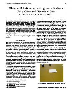
4. Visualization Radar reflections come from various objects in a scene. By visualizing the information about the clusters extracted by the above method, we can easily understand the objects, e.g. their nature, location, and velocity. As shown in Fig.3, the clusters in every radar frame are visualized by drawing semitransparent rectangles on the
�
�
�
Object position — Rectangle position, which is decided by the transformed position of the cluster. Distance to the object — Rectangle height, which is decided by a value that is inversely proportion to the distance of the cluster. Object width — Rectangle width, which is decided by the left-most and right-most signals of the cluster. Relative velocity of the object — Length and direction of an arrow at the lower part of the rectangle; the length is determined by the relative velocity of the cluster, while upward and downward arrows represent leaving and approaching objects, respectively.
5. Experimental Results We mount the radar and the camera at the front of the vehicle as shown in Fig.4. This section presents a calibration result between the sensors along with segmentation and visualization results using real radar/image frame sequences observed in urban areas.
5.1. Calibration Fig. 5(a) shows an example of the intensity sequence described in Section 2. The 46 data sets, which represent positions on the radar plane and the image plane, are shown in Fig. 5(b) and Fig. 5(c), respectively. We estimated the homography matrix H using the data sets. Fig.5(d) shows transformed positions (the radius between 10–50m and the angle between -10–10˚) on the radar plane to the image plane using the H. Fig.5(a) indicates that the radar fails to acquire the correct reflection intensity of the reflector at some frames, which represents the lacking stability of radar observation. Extracted points on both planes are influenced by the lacking stability. However, the calibration result in Fig.5(d) reasonably indicates the actual sensors’ arrangement, i.e. the radar is located above the camera, and scanning directions of the radar are nearly parallel to the y axis of the image.
0-7695-2128-2/04 $20.00 (C) 2004 IEEE
power 200
y[m] 10
180
8
160
6
140
4
120
2
100 250
300
350
400
450
500 frames
(a) intensity sequence y[pix] 450 400 350 300 250 200 150 100 50 0 0
0 -3
07 08 09 10 11 12 13 14
-2
-1
0
1
2
3 x[m]
(b) calibration points (radar)
y[pix] 450 400 350 300 250 200 150 100 50 500 600 0 0 x[pix] 07 08 09 10 11 12 13 14
100
200
300
400
(c) calibration points (image)
Figure 6. Segmentation and visualization (Scene 1) -10q
0q
10q
10[m] 20[m] 30[m] 40[m] 50[m]
100
200
300
400
500
600 x[pix]
(d) calibration result
Figure 5. Calibration result Figure 7. Segmentation and visualization (Scene 2)
5.2. Segmentation and Visualization Fig. 6 and 7 show examples of acquired radar/image frames for low speed driving in urban areas. Each left figure shows acquired radar data and segmentation results (clusters are indicated by ellipses) in Cartesian coordinates. Each corresponding image frame to the radar frame is shown on the right. Two vertical lines on the left and right parts of the image frame indicate the right-most and the left-most limits of the radar’s scanning angle, respectively. We processed radar data which were within 30m of the vehicle. In the image of Fig.6, there are four vehicles (leaving, standing, and two oncoming). Their radar reflections are divided into clusters correctly; the clusters are visualized effectively on the image. The arrows at the lower part of the rectangles indicate the correct direction and relative velocity of the objects. In the image of Fig.7, three objects (a parked vehicle, a walking girl, an obstacle) are also detected and visualized satisfactorily. In the image frame of Fig.6, the cluster of the standing vehicle seems too wide; this results from the low directional resolution of the radar. If the larger threshold of signal intensity is defined for removing noise, the cluster’s width could be made smaller. However, we use a small threshold because reflection intensities from pedestrians are relatively weak and the small data number in the cluster tends to cause tracking error. Visualization results show that the positions of the clusters, which are transformed on the images by the homography matrix H, do not always represent the correct objects’ position on the image. However, by visualization of the cluster’s information, we can easily understand not only its
position, relative velocity, and size, but what exists there.
6. Summary and Future Work We proposed a calibration method between millimeterwave radar and a CCD camera using homography. We also segmented radar data into clusters and visualized them on an image sequence. In experimental results, we obtained a good calibration result and the clusters were segmented and visualized effectively on images. Observation errors in radar data increase especially at low speed driving in crowded areas. Therefore, image processing approaches such as region and/or motion segmentation would be necessary for accurate obstacle detection for urban driving. Future work will develop sensor fusion techniques using these proposed calibration method and the image processing approaches.
References [1] Aufrere R., Mertz C. and Thorpe C., “Multiple Sensor Fusion for Detecting Location of Curbs, Walls, and Barriers,” IEEE Intelligent Vehicle Symposium, pp. 126–131, 2003 [2] Mockel S., Scherer F. and Schuster P.F, “Multi-Sensor Obstacle Detection on Railway Tracks,” IEEE Intelligent Vehicle Symposium, pp. 42–46, 2003 [3] Meis U. and Schneider R., “Radar Image Acquisition and Interpretation for Automotive Applications,” IEEE Intelligent Vehicles Symposium, pp. 328–332, 2003
0-7695-2128-2/04 $20.00 (C) 2004 IEEE