Apr 4, 2017 - plicit surface representation from the input depth maps. Our learning ... of affordable depth sensors, in particular the Microsoft. Kinect sensor ...
OctNetFusion: Learning Depth Fusion from Data Gernot Riegler1 Ali Osman Ulusoy2 Horst Bischof1 Andreas Geiger2,3 1 Institute for Computer Graphics and Vision, Graz University of Technology 2 Autonomous Vision Group, MPI for Intelligent Systems T¨ubingen 3 Computer Vision and Geometry Group, ETH Z¨urich
arXiv:1704.01047v1 [cs.CV] 4 Apr 2017
{riegler, bischof}@icg.tugraz.at
{osman.ulusoy,andreas.geiger}@tue.mpg.de
Abstract In this paper, we present a learning based approach to depth fusion, i.e., dense 3D reconstruction from multiple depth images. The most common approach to depth fusion is based on averaging truncated signed distance functions, which was originally proposed by Curless and Levoy in 1996. While this method achieves great results, it can not reconstruct surfaces occluded in the input views and requires a large number frames to filter out sensor noise and outliers. Motivated by large 3D model databases and recent advances in deep learning, we present a novel 3D convolutional network architecture that learns to predict an implicit surface representation from the input depth maps. Our learning based fusion approach significantly outperforms the traditional volumetric fusion approach in terms of noise reduction and outlier suppression. By learning the structure of real world 3D objects and scenes, our approach is further able to reconstruct occluded regions and to fill gaps in the reconstruction. We evaluate our approach extensively on both synthetic and real-world datasets for volumetric fusion. Further, we apply our approach to the problem of 3D shape completion from a single view where our approach achieves state-of-the-art results.
(a) TSDF Fusion [9]
(b) Our Approach
Figure 1: Depth fusion results using four uniformly spaced views around the object. (a) TSDF fusion produces noisy and incomplete results for small number of input views. (b) Our learning based approach leverages large 3D model databases and 3D CNNs to significantly improve fusion results in terms of noise reduction and surface completion.
from 2.5D depth images remains a difficult problem. Challenges include sensor noise, quantization artifacts, outliers (e.g., bleeding at object boundaries) and missing data such as occluded surfaces. Some of these challenges can be addressed by integrating depth information from multiple viewpoints in a volumetric representation. In particular, Curless and Levoy demonstrate that averaging truncated signed distance functions (TSDF) allows for a simple yet effective approach to depth fusion [9]. More than a decade later its introduction, state of the art 3D reconstruction methods such as Newcombe et al. [31] and a large body of follow-up works [6, 32, 46, 49] rely on TSDF fusion. While TSDF fusion is utilized widely in the community, it has two major drawbacks. First, it requires a large number of frames to smooth out the sensor noise and outliers. Second, it can not reconstruct occluded regions or complete large holes. In this paper, we tackle these problems by proposing a learning-based solution to volumetric fusion. By utilizing large datasets of 3D models and high capacity 3D convolutional neural networks (3D CNNs), our approach learns to smooth out sensor noise, deals with outliers as well as completes missing 3D geometry. To the best of our knowledge, our approach is the first to learn volumetric fusion
1. Introduction Reconstructing accurate and complete 3D surface geometry is a core problem in computer vision. While image based techniques [12, 15, 39, 40, 48] provide compelling results for sufficiently textured surfaces, the introduction of affordable depth sensors, in particular the Microsoft Kinect sensor, allows scanning a wide variety of objects and scenes. This has led to the creation of large databases of real-world 3D content [7, 10, 42, 43], enabling progress in a variety of areas including 3D modeling [28, 52], 3D reconstruction [6, 50], 3D recognition [18, 44] and 3D scene understanding [16, 42]. However, creating complete and accurate 3D models 1
from noisy depth observations. 3D CNNs [8, 22, 28, 34, 51] are a natural choice for formulating this task as an end-to-end learning problem. However, existing deep learning approaches are limited to small resolutions (typically 323 voxel grids) due to the cubic growth in memory requirements. A notable exception is the OctNet approach of Riegler et al. [36]. Their approach takes advantage of the sparsity of 3D volumetric models using an octree representation [37], enabling deep learning at resolutions of 2563 voxels and beyond. The main limitation of OctNets, however, is that the octree representation is derived from the input and fixed during learning and inference. While this is sufficient for tasks such as 3D semantic segmentation where the input and the output share the same octree representation, it is not applicable to tasks where the 3D space partitioning of the output is unknown a priori and may be different than that of the input. For instance, for tasks such as depth map fusion and 3D completion, the input and output octrees might be dramatically different as the location of the implicit surface is unknown and needs to be inferred from noisy observations. The key contribution of this paper is to lift this restriction. More specifically, we propose a novel 3D CNN architecture termed OctNetFusion which takes as input one or more depth images and estimates both the complete 3D reconstruction and its 3D space partitioning, i.e. the output octree structure. By decoupling the input and output octree structures, our approach allows for reconstructing 3D models that have significantly different space partitioning from the input. We apply this architecture to the depth map fusion problem and formulate the task as the prediction of truncated signed distance fields which can be meshed using standard techniques [27]. We evaluate our approach on synthetic and real-world datasets, studying several different input and output representations, including the TSDF. Our experiments demonstrate that the proposed method is able to reduce noise and outliers compared to TSDF fusion [9, 31]. Besides, our model learns to complete missing surfaces and fill holes in the reconstruction. We further demonstrate the flexibility of our model by evaluating it on the task of volumetric shape completion from a single view where we obtain improvements wrt. the state-of-the-art [14]. Our code and data will be made available upon acceptance.
2. Related Work Volumetric Fusion: In their seminal work, Curless and Levoy [9] proposed to integrate range information across viewpoints by averaging truncated signed distance functions. The simplicity of this method has turned it into a universal approach that is used in many 3D reconstruction pipelines. Using the Microsoft Kinect sensor and GPGPU
processing, Newcombe et al. [31] showed that real-time 3D modeling is feasible using this approach. Large-scale 3D reconstruction has been achieved using iterative re-meshing [49] and efficient data structures [32, 46]. The problem of calibration and loop-closure detection has been considered in [6, 55]. Due to the simplicity of the averaging approach, however, these methods typically require a large number of input views, are susceptible to outliers in the input and don’t allow to predict surfaces in unobserved regions. Noise reduction can be achieved using variational techniques which integrate local smoothness assumptions [2,19, 53] into the object. However, those methods are typically slow and can not handle missing data. In this paper we propose an alternative learning based approach which is both fast and allows for surface completion. Ray Consistency: While TSDF fusion does not explicitly consider free space and visibility constraints, ray potentials allow modeling these constraints in a Markov random field. Ulusoy et al. [47, 48] consider a fully probabilistic model for image based 3D reconstruction. Liu and Cooper [26] formulate the task as MAP inference in a Markov random field. In contrast to our method, these algorithms do not learn the geometric structure of objects and scene from data. Instead, they rely on simple hand-crafted priors such as spatial smoothness [26], or piecewise planarity [47]. Notably, Savinov et al. combine ray potentials with 3D shape regularizers that are learned from data [38]. Their approach relies on an input semantic segmentation. In this work, we do not consider the semantic class of the reconstructed object or scene and focus on the generic 3D reconstruction problem. Shape Completion: If exact 3D models are available, missing surfaces can be completed by detecting the objects and fitting 3D models to these observations [3, 20]. In this paper, we assume that such prior knowledge is not available. Instead we directly learn to predict the 3D structure from training data in an end-to-end fashion. Shape completion from a single RGB-D image by reasoning in 3D voxel space has been tackled in [14,23,45,54]. While [23] use a CRF for inference, [14] predict structured outputs using a random forest and [45] use a CNN to jointly estimate voxel occupancy and semantic class labels. In contrast to our approach, these methods reason at the voxel level and therefore do not provide sub-voxel surface estimates. Furthermore, 3D CNN based methods [45] are limited in terms of resolution. In this paper, we demonstrate a unified approach which allows to reason about missing 3D structures at large resolution while providing sub-voxel surface estimates. In contrast to single-image reconstruction methods, our approach handles an arbitrary number of input views. We provide a comparison to [14] on the task of single image shape completion in addition to the volumetric fusion experiments which are our main focus.
In very recent work, Dai et al. [11] consider the problem of high-resolution 3D shape completion. Their approach first regresses 323 voxel volumes using a 3D CNN, followed by a multi-resolution 3D shape synthesis step using a large database of 3D CAD models [5]. While their objectcentric approach is able to reconstruct details of individual objects with known 3D shape, we put our focus on general 3D scenes where such global knowledge is generally not available.
the number of voxels comprised by this cell. If the cell is at the finest resolution of the tree, we have |Ω[i, j, k]| = 1, i.e., the cell is equal to the voxel in Ti,j,k . In contrast, if the complete shallow octree consists of only a single leaf cell, then |Ω[i, j, k]| = 512 as all 83 voxels are pooled. Given this basic notation, the authors of [36] show how the convolution, pooling and unpooling operation can be efficiently implemented on this data structure.
3.2. OctNetFusion
3. OctNetFusion This section introduces our OctNetFusion architecture. As our work extends [36] we follow their notation whenever possible. To make this paper self-contained, we first briefly review OctNet [36] in Section 3.1. Then, we present our OctNetFusion approach in Section 3.2 which learns to jointly estimate the output quantity (e.g., signed distance or occupancy) and the space partitioning to focus computations where needed. Finally, in Section 3.3, we specify the input and output representations which we evaluate in our experimental evaluation.
3.1. OctNet The main limitation of conventional 3D CNNs that operate on regular voxel grids is the cubic growth in memory requirements with respect to the voxel resolution. However, 3D data is often sparse in nature [25]. For instance, the surface of an object can be interpreted as a 2D manifold in 3D space. Riegler et al. [36] utilize this observation and define a convolutional neural network on the efficient grid-octree data structure of [29]. The data structure itself consists of a grid of shallow octrees with maximum depth D = 3, trading off computation and memory. The structure of the shallow octrees can be efficiently encoded as bit strings that allows for rapid retrieval of neighboring cells. One important property of OctNets is that none of the operations (i.e., convolution, pooling, unpooling) changes the grid-octree data structure which is based on the input (e.g., point cloud, voxel grid). This can be seen as a data-adaptive pooling operation which maps the output of each layer back to the grid-octree representation. We now introduce the basic notation. Consider a dense voxel grid T ∈ R8D×8H×8W where Ti,j,k denotes the value at voxel (i, j, k). Further, let O denote a grid-octree data structure that covers the same volume. Given tree depth of D = 3 this data structure would contain D×H ×W shallow octrees, where each shallow octree covers 83 voxels. The important difference to the dense representation is that the cells in O can comprise a variable number of voxels. Let Ω[i, j, k] denote the smallest grid-octree cell that contains the voxel at (i, j, k). Ω[i, j, k] can be interpreted as the set of voxel indices, whose data is pooled to a single value as described above. Furthermore, |Ω[i, j, k]| denotes
The main drawback of OctNet as proposed in [36] is that the octree structure of the input and the output, i.e. the partitioning of the 3D space, has to be known a priori. This is a reasonable assumption for tasks like 3D point cloud labeling (e.g., semantic segmentation) where the input and the output octree structures are the same. However, for tasks where the output geometry is different from the input geometry, e.g., in volumetric fusion or shape completion, the grid-octree data structure has to be adapted during inference. We now present our OctNetFusion architecture, illustrated in Fig. 2, which allows to learn the grid-octree structure along with the 3D task in a principled manner. Network Architecture: Our overall network architecture is illustrated in Fig. 2a. We represent the voxelized input and output using the grid-octree structure described in Section 3.1. The input to the network is calculated based on a single depth map or by fusing information from multiple depth maps. The output may encode a TSDF or a binary occupancy map, depending on the application. We refer the reader to Section 3.3 for all necessary details. As the 3D input to our method can be sparse and incomplete, we refrain from using the classical U-shaped architecture as common for 2D-to-2D prediction tasks [1, 13]. Instead, we propose a coarse-to-fine network with encoderdecoder modules, structure manipulation modules and a loss defined at every pyramid level. More specifically, we create a 3D scale pyramid where the number of voxels along each dimension increases by a factor of two between pyramid levels. At each level, we process the input using an encoder-decoder module which enlarges the receptive field and captures contextual information. We pass the resulting features to a structure manipulation module which computes the output at the respective resolution, increases the resolution and updates the structure of the network for further processing. We propagate features to successively finer resolutions until we have reached the final target resolution. We will now describe the encoder-decoder module and the structure module in detail. Encoder-Decoder Module: The encoder-decoder module is illustrated in Fig. 2b. It combines convolution layers with pooling and unpooling layers similar to the segmentation
∆
∆
conv ◦ concat
1
N
16
32
64
64
16
1
N
16
32
32
32
64
64
64
643
unpool
conv ◦ concat 32
64
16
16
1
conv ◦ concat 32
32
32
64
pool
64
pool
pool
unpool
conv ◦ concat 32
conv ◦ concat
16
pool
16
pool
pool
16
pool
32
pool
pool
16
64
64
1283
unpool
conv ◦ concat
N
∆
64
32
32
64
2563
(a) Network Architecture conv ◦ concat 32
pool
16
pool
N
Pn2D×2H×2W
unpool 16
16
split
Q2D×2H×2W n
1
pool
unpool
conv ◦ concat 32
64
64
64
32
32
OnD×H×W
convm,1
R1D×H×W
∆
64
(b) Encoder-Decoder Module
(c) Structure Module
Figure 2: OctNetFusion Architecture. (a) Overall structure of our network. (b) Encoder-decoder modules increase the receptive field size and add contextual information. (c) Structure manipulation modules increase the spatial resolution of the feature maps. A loss at the end of each pyramid level measures the quality of the reconstruction at the respective resolution. network used in [36]. All convolutional layers are followed by a ReLU non-linearity [30]. Each pooling operation doubles the number of feature maps while each unpooling operation halves the number of features. Pooling operations reduce spatial information but increase the level of semantics and context captured in the features. The result of the unpooling operation is concatenated with the corresponding high-resolution features from the encoder path to combine high-resolution information with low-resolution contextual cues. Structure Module: As discussed above, the unpooling operation of the original OctNet architecture [36] has one major drawback: the grid-octree structure must be known in advance to determine which voxels shall be split. While for the task of point cloud labeling the structure can be split according to the input, the final output structure is unknown for tasks like volumetric fusion or completion. Na¨ıvely splitting all voxels would eliminate the advantage of the data-adaptive representation and limit the output resolution to small volumes. Consequently, we introduce a structure module after each encoder-decoder module which determines for each voxel if it shall be split (i.e., close to the surface) or not (i.e., far from the surface). Our structure module is illustrated in Fig. 2c. The main idea is to add a split mask to the standard unpooling operation that indicates which of the octree cells should be further subdivided. This splitting mask is then used to subdivide the unpooled grid-octree structure. More formally, let us consider an input grid-octree struc-
(a) Before Split
(b) After Split
Figure 3: Cell Splitting. The structure module splits each cell based on its distance from the implicit surface.
ture O with n feature channels and D × H × W shallow octrees. After the unpooling operation we obtain a structure P that consists of 2D × 2H × 2W shallow octrees, but all octree cells comprise eight-times the number of voxels, i.e., |ΩP [2i, 2j, 2k]| = 8|ΩO [i, j, k]|. Additionally, we output a reconstruction R at the resolution of O using a single convolution followed by a sigmoid non-linearity or a 1 × 1 convolution depending on the desired output (occupancy or TSDF, respectively). The reconstruction output is used by our multi-scale reconstruction loss to predict a correct reconstruction at each resolution of the network. We define the split mask implicitly by the surface of the reconstruction R. The surface is defined by the gradients of R when predicting occupancies or by the zero-levelset of
R in the case of TSDF regression. Given the surface, we split all voxels within distance τ from the surface as illustrated in Fig. 3. For TSDF regression, τ equals the truncation threshold. For occupancy classification, τ is a flexible parameter which can be tuned to trade accuracy vs. memory usage. The output of this split operation finally yields the higher-resolution structure Q which serves as input to the next level.
3.3. Input / Output Encoding This section describes the input and output encodings for our method. An ablation study, analyzing the individual encodings is provided in Section 4. 3.3.1
Input Encoding
The input to our method are one or more 2.5D depth maps. We now discuss several ways to map these 2.5D inputs into 3D voxel space which, represented using grid-octree structures, forms the input to the OctNetFusion architecture described above. The traditional volumetric fusion approach [9] calculates the weighted average TSDF with respect to all depth maps independently for every voxel where the distance to the surface is measured along the line of sight to the sensor. While providing for a simple one-dimensional signal at each voxel, this encoding might result in a loss of information since TSDF values are averaged. Thus, we also explore higher dimensional input encodings which might better retain the information present in the sensor recordings. We now formalize all input encodings used during our experiments, starting with the simplest one. Occupancy Fusion (1D): The first, and simplest encoding (i) fuses information at the occupancy level. Let dv be the (i) depth of the center of voxel v wrt. camera i. Further, let dc be the value of the depth map when projecting voxel v onto the image plane of camera i. Denoting the signed distance (i) (i) (i) between the two depth values as δv = dc −dv , we define the occupancy of each voxel o(v) as ( (i) (i) 1 ∃i : δv ≤ s ∧ @i : δv > s o(v) = (1) 0 else where s is the size of voxel v. This definition has the following simple interpretation: If there exists any depth map in which voxel v is observed as free space the voxel is marked as free, otherwise it is marked as occupied. While simple, this input encoding is susceptible to outliers in the depth maps and doesn’t encode uncertainty. Furthermore, the input distance values are not preserved as only occupancy information is encoded. Occupancy Accumulators (3D): Our second input encoding is inspired by Hu et al. [21] who proposed free space and
occupancy accumulators for probabilistic occupancy mapping. Differently from them, we use a three-dimensional encoding which captures free space, surface and unknown regions in separate channels and exploit this information for training our OctNetFusion architecture. More specifically, we consider three accumulators for each voxel which we represent by the vector a(v) ∈ R3 . After initializing a(v) = 0, we update a(v) for each camera view i using: (1, 0, 0) (0, 1, 0) a(v) = a(v) + (0, 0, 1) (0, 0, 0)
(i)
δv > s (i) δv < s (i) |δv | ≥ s (i) δv = invalid
(2)
After accumulation, we normalize a(v) to ka(v)k1 = 1. Compared to “Occupancy Fusion”, this encoding is more robust to noise and captures uncertainty in the inputs. For example, if a(v) = (1, 0, 0)T all views agree on free space while a(v) = ( 31 , 13 , 13 )T indicates conflicting information. However, distance values are not preserved. TSDF Fusion (1D): Our third input encoding is traditional TSDF fusion as described by [9, 31]. To compute this encoding, we project the center of each voxel into every depth map, calculate the truncated signed distance using a truncation threshold τ (corresponding to the size of four voxels in all our experiments), and average the result over all input views. While various weight profiles have been proposed [46], we found that the simple constant profile proposed by Newcombe et al. [31] yields good performance. This input representation is simple and preserves distance values, but it does not encode uncertainty and therefore makes it harder for the network to resolve conflicts. Accumulators + TSDF Fusion (4D): We consider a combination of the TSDF and accumulator encodings where the three-dimensional “Occupancy Accumulators” is simply concatenated with the one-dimensional “TSDF Fusion” encoding, yielding a 4D input encoding which captures both the predicted distance to the surface, as well as the uncertainty about this prediction. Histogram (ND): While the previous encoding captures surface distance and uncertainty, it does not maintain the multi-modal nature of fused depth measurements. To capture this information, we propose a histogram-based representation. In particular, we encode all distance values for each voxel using a ND histogram with 10 bins for negative and 10 bins for positive distance values. In particular, the first and the last bin of the histogram capture distance values beyond the truncation limit, while the bins in between collect non-truncated distance values. To allow sub-voxel surface estimation, we choose the histogram size such that a minimum of 2 bins are allocated per voxel. Furthermore,
we populate the histogram in a smooth fashion by distributing the vote of each observation linearly between the two closest bins, e.g., we assign half of the mass to both neighboring bins if the prediction is located at their boundary.
643 1283 2563
Fusion
Occ.
Acc.
TSDF
TSDF+Acc.
Hist.
19.442 11.366 6.214
9.643 5.052 2.824
9.247 4.744 2.562
8.789 4.256 2.458
8.930 4.818 2.870
8.224 4.148 2.484
(a) MSE (mm)
3.3.2
Output Encoding & Loss
Finally, we describe the output encodings and the loss we use for the volumetric fusion and the volumetric completion tasks we consider in the experimental evaluation. Volumetric Fusion: For volumetric fusion, we choose the TSDF as output representation using an appropriate truncation threshold τ . We regress the TSDF values at each resolution (i.e., within the structure module) using a 1 × 1 convolution layer and use the `1 loss for training. Volumetric Completion: For volumetric completion from a single view, we are only interested in the voxel-level output of our network. Consequently both the TSDF as well as the binary occupancy representation are applicable to this task. In our volumetric completion experiments, we use the binary occupancy representation to match the setup of the baselines as closely as possible. For training, we use the binary cross entropy loss.
4. Evaluation In this section, we present our experiments and evaluations. In Section 4.1 we consider the task of volumetric fusion from multiple depth images and in Section 4.2 we compare our approach to a state-of-the-art baseline on the task of volumetric completion, i.e. 3D reconstruction from a single depth image.
4.1. Volumetric Fusion In this section we consider the volumetric fusion task. We evaluate our OctNetFusion approach on the synthetic ModelNet40 dataset of Wu et al. [52] as well as on real Kinect object scans that are generated using the depth image dataset by Choi et al. [7]. Unfortunately, the ground truth TSDF can not be calculated directly from the 3D models in ModelNet as the meshes are not watertight, i.e., they contain holes and cracks. Moreover, the meshes typically do not have consistently oriented normals. Instead, we obtain ground truth TSDF by sampling views around the object densely and uniformly from a sphere, render the input 3D model from these views and run traditional volumetric fusion on those generated depth maps. We found that 80 view points allow computing high accuracy TSDF ground truth. We selected 10 model categories and for each category used 200 models for training and 20 for testing from the provided train/test split, respectively.
643 1283 2563
Fusion
Occ.
Acc.
TSDF
TSDF+Acc.
Hist.
5.183 2.561 1.259
2.287 0.912 0.717
2.286 0.862 0.445
2.334 0.758 0.571
2.704 0.984 0.520
2.554 1.010 0.388
(b) SAD (mm) 643 1283 2563
Fusion
Occ.
Acc.
TSDF
TSDF+Acc.
Hist.
0.638 0.567 0.548
0.734 0.753 0.751
0.762 0.778 0.776
0.777 0.798 0.792
0.773 0.767 0.763
0.777 0.799 0.776
(c) Jaccard Index
Table 1: Evaluation of Different Input Encodings
Besides the synthetic ModelNet dataset, we also evaluate our approach on real depth sensor data. In particular, we use depth images distributed by Choi et al. [7] which includes a diverse set of objects such as chairs, tables, trash containers, plants, signs, etc. Unfortunately, the dataset does not include ground-truth 3D models or camera poses. We estimate the camera poses using Kintinuous [49] and visually inspect all models to remove those for which the pose tracking failed. We use TSDF fusion to obtain approximate ground-truth 3D models. We found that the high number of frames (roughly 1000 frames for each object) allows computing an high quality ground-truth. Example ground-truth 3D models are shown in Fig. 4. Note that as input to our method, we use two to three orders of magnitude less images in our experiments. We collected a total of 85 scenes, where we randomly selected 10 for the evaluation. Additionally, we augment the dataset by generating 20 different view configurations per scene by selecting different and disjoint subsets of view points. In the following, we provide experiments analyzing the effect of different input encodings, number of views and the generalization ability of our model. Additional experiments can be found in the supplementary material. Input Encoding: We first investigate the impact of the input encodings discussed in Section 3.3.1 on the quality of the output. We scaled the models to fit into a cube of 3×3×3 meters and rendered the depth maps onto 4 equally spaced views on a sphere as input. To simulate a realistic environment, we artificially added depth dependent Gaussian noise [33]. We provide sample depth maps in the supplementary document. Our results are shown in Table 1 which compares the traditional volumetric fusion approach [9] (left column) to
Fusion1 643 1283 2563
100.331 52.231 26.704
Ours1
Fusion2
33.896 18.309 9.462
43.388 23.779 12.533
Ours2 14.347 7.702 4.294
Fusion4 19.442 11.366 6.214
Ours4 8.789 4.256 2.458
(a) MSE (mm) 643 1283 2563
Fusion1
Ours1
Fusion2
Ours2
Fusion4
Ours4
62.995 31.637 15.837
12.002 5.579 2.779
17.053 8.551 4.272
4.083 1.695 0.951
5.183 2.561 1.259
2.334 0.758 0.571
(b) SAD (mm) 643 1283 2563
643
Fusion
Class Aware
Class Agnostic
airplane
1283 2563
7.694 5.180 3.007
3.957 1.403 0.771
2.973 1.350 0.736
car
643 1283 2563
18.323 11.132 6.135
11.373 6.420 3.480
10.560 6.301 3.392
chair
643 1283 2563
16.548 9.844 5.473
9.014 4.406 2.157
7.290 3.590 1.902
(a) MSE (mm)
Fusion1
Ours1
Fusion2
Ours2
Fusion4
Ours4
0.136 0.132 0.130
0.361 0.370 0.363
0.372 0.336 0.328
0.642 0.692 0.681
0.638 0.567 0.548
0.777 0.798 0.792
Table 3: Class Aware vs. Class Agnostic Networks
(c) Jaccard Index
Table 2: Evaluation wrt. Number of Input Views Figure 4: Examples from Kinect Scan Dataset our learned approach using the input encodings described in Section 3.3.1. We evaluate our results in terms of three different metrics: (a) mean squared error (MSE) in millimeters, (b) sum of absolute differences (SAD) in millimeters, and (c) Jaccard Index which measures the intersection-overunion of the voxels classified as occupied (i.e., voxels behind the surface). Each row shows results at a particular resolution, ranging from 643 to 2563 . First, we observe that our approach outperforms the traditional fusion approach in all metrics for all resolutions. Improvements are particularly pronounced at high resolutions which demonstrates that our learning based approach is able to refine and complete geometric details which can not be recovered using the standard fusion approach. Furthermore, we observe that the TSDF and the histogram encoding lead to the best results with similar performance. We conclude that the additional per-view information provided by the accumulator or the histogram encoding are not significant for the volumetric fusion task and that this information is implicitly present in the input TSDF. We thus use the TSDF input encoding for all experiments that follow. Number of Views: Next, we evaluate the performance of our network when varying the number of input views from one (Fusion1 /Ours1 ) to four (Fusion4 /Ours4 ) using the same dataset and setting as described in the previous section and the TSDF as input encoding. Our results are shown in Table 2. Again, our approach outperforms the traditional fusion approach in all categories and at all resolutions. As expected, performance increases with the number of viewpoints. The largest difference between the baseline and our approach is visible for the experiment with only one input view. While no fusion is performed in this case, this demonstrates that our learned model is effective in complet-
ing missing geometry. For four input views, our approach reduces errors by a factor of 2 to 3. Class Aware vs. Class Agnostic: Most existing approaches that leverage deep learning for 3D reconstruction train a model specific for a particular object class [4, 8, 17, 35, 41] which typically does not generalize well to other classes or scenes with varying backgrounds as present in our Kinect experiments using the scans of Choi et al. [7]. In contrast, here we are interested in 3D reconstruction of general scenes. We therefore analyze how our model behaves when trained and tested on a single class and compare the results to a model trained on all classes and tested on a single class. We show our results for the object categories “airplane”, “car” and “chair” in Table 6. Due to space limitations, we only show the MSE metric, the other results can be found in the supplementary material. Surprisingly, we observe that in all cases, the class agnostic model outperforms the class aware model. We conclude that the number of training examples, which is significantly lower for the class aware training, is more important than training a class specific networks. Moreover, this experiment shows that our approach generalizes well to novel categories. Qualitative Results on ModelNet: We show qualitative results on ModelNet in Fig. 5 using the TSDF encoding and 4 views. The same TSDF truncation threshold has been used for traditional fusion, our OctNetFusion approach and the ground truth generation process. While the baseline approach is not able to resolve conflicting TSDF information from different viewpoints, our approach learns produce a smooth and accurate 3D model from highly noisy input. Kinect Object Scans: To evaluate the performance of our
Ours
Ground Truth
Fusion
Ours
Ground Truth
2563
2563
1283
1283
643
643
Fusion
(b) Bed
(a) Airplane
Figure 5: Qualitative Results on ModelNet using 4 equally spaced viewpoints
Fusion10 Ours10 Fusion20 Ours20 Fusion50 Ours50 643 1283 2563
135.654 77.696 42.928
50.977 26.247 11.791
101.536 59.801 33.986
45.756 23.728 10.624
64.678 39.084 23.185
36.422 19.113 9.551
(a) MSE (mm) Fusion10 Ours10 Fusion20 Ours20 Fusion50 Ours50 643 1283 2563
90.922 51.908 28.447
29.654 13.119 4.908
60.997 35.299 19.611
25.646 11.476 4.602
33.481 19.603 11.072
18.853 8.673 3.867
(b) SAD (mm) Fusion10 Ours10 Fusion20 Ours20 Fusion50 Ours50 643 1283 2563
0.423 0.293 0.196
0.688 0.536 0.446
0.530 0.388 0.271
0.719 0.631 0.519
0.678 0.539 0.403
0.771 0.685 0.593
(c) Jaccard Index
Table 4: Fusion of Kinect Object Scans algorithm on real data, we use the dataset of Kinect object scans published by Choi et al. [7]. For this experiment we vary the number of input views from ten (Fusion10 /Ours10 ) to fifty (Fusion50 /Ours50 ) as the scenes are larger and the camera trajectories are less regular than in the synthetic ModelNet experiments. Our results are shown in Table 4. While overall errors are larger compared to the ModelNet experiments, we again outperform the traditional fusion approach at all resolutions and for all number of input views. Notably, the relative difference between the two methods increases with finer resolution which demonstrates the impact of learned representations for reconstructing details. Due to space limitations we provide qualitative results in the supplementary material.
Method
IoU
Precision
Recall
Zheng et al. [54]* Voxlets et al. [14]*
0.528 0.585
0.773 0.793
0.630 0.658
Voxlets et al. [14] Ours
0.550 0.650
0.734 0.834
0.705 0.756
Table 5: Volumetric Completion (Tabletop). The numbers marked with asterisk (*) are taken from [14] while the others have been recomputed by us and verified by the authors of [14]. Unfortunately, even in a joint effort with the authors, we were not able to reproduce the original results due to irreversible post-publication changes in their dataset, thus we provide both results in this table.
4.2. Volumetric Completion In this section, we provide a comparison to Firman’s Voxlets approach et al. [14] on the task of volumetric shape completion from a single image. For this experiment, we use the dataset and metrics proposed by [14] and modify our model to predict binary occupancy maps instead of realvalued TSDFs. Our results are shown in Table 5. As evidenced by our results, our approach improves upon Voxlets [14] as well as the method of Zheng et al. [54] in terms of intersection-over-union (IoU) of the occupied space, precision and recall. Unfortunately, even after communication with the authors we were not able to reproduce their results due to post-publication changes in their dataset. However, the authors promised to fix these problems after the ICCV17 deadline and we will upate the final version of this paper accordingly.
5. Conclusion We propose OctNetFusion, a deep 3D convolutional neural network that is capable of fusing depth information from
different viewpoints to produce accurate and complete 3D reconstructions. Our experiments demonstrate the advantages of our learning-based approach over the traditional fusion baseline and shown that our method generalizes to novel object categories and produces compelling results on synthetic and real Kinect data. While in this paper we have focused on the depth map fusion problem, an interesting direction is to extend our model to 3D reconstruction from RGB images where 3D representations are learned jointly with 2D image representations in an end-to-end fashion.
References [1] V. Badrinarayanan, A. Kendall, and R. Cipolla. Segnet: A deep convolutional encoder-decoder architecture for image segmentation. arXiv.org, 1511.00561, 2015. 3 [2] M. Blaha, C. Vogel, A. Richard, J. D. Wegner, T. Pock, and K. Schindler. Large-scale semantic 3d reconstruction: An adaptive multi-resolution model for multi-class volumetric labeling. In Proc. IEEE Conf. on Computer Vision and Pattern Recognition (CVPR), 2016. 2 [3] E. Brachmann, A. Krull, F. Michel, S. Gumhold, J. Shotton, and C. Rother. Learning 6d object pose estimation using 3d object coordinates. In Proc. of the European Conf. on Computer Vision (ECCV), 2014. 2 [4] A. Brock, T. Lim, J. M. Ritchie, and N. Weston. Generative and discriminative voxel modeling with convolutional neural networks. arXiv.org, 1608.04236, 2016. 7 [5] A. X. Chang, T. A. Funkhouser, L. J. Guibas, P. Hanrahan, Q. Huang, Z. Li, S. Savarese, M. Savva, S. Song, H. Su, J. Xiao, L. Yi, and F. Yu. Shapenet: An information-rich 3d model repository. arXiv.org, 1512.03012, 2015. 3 [6] S. Choi, Q. Zhou, and V. Koltun. Robust reconstruction of indoor scenes. In Proc. IEEE Conf. on Computer Vision and Pattern Recognition (CVPR), 2015. 1, 2 [7] S. Choi, Q. Zhou, S. Miller, and V. Koltun. A large dataset of object scans. arXiv.org, 1602.02481, 2016. 1, 6, 7 [8] C. B. Choy, D. Xu, J. Gwak, K. Chen, and S. Savarese. 3dr2n2: A unified approach for single and multi-view 3d object reconstruction. In Proc. of the European Conf. on Computer Vision (ECCV), 2016. 2, 7 [9] B. Curless and M. Levoy. A volumetric method for building complex models from range images. In ACM Trans. on Graphics (SIGGRAPH), 1996. 1, 2, 5, 6 [10] A. Dai, A. X. Chang, M. Savva, M. Halber, T. Funkhouser, and M. Niessner. Scannet: Richly-annotated 3d reconstructions of indoor scenes. In Proc. IEEE Conf. on Computer Vision and Pattern Recognition (CVPR), 2017. 1 [11] A. Dai, C. R. Qi, and M. Nießner. Shape completion using 3d-encoder-predictor cnns and shape synthesis. In Proc. IEEE Conf. on Computer Vision and Pattern Recognition (CVPR), 2017. 2 [12] A. Delaunoy and M. Pollefeys. Photometric bundle adjustment for dense multi-view 3d modeling. In Proc. IEEE Conf. on Computer Vision and Pattern Recognition (CVPR), 2014. 1
[13] A. Dosovitskiy, P. Fischer, E. Ilg, P. Haeusser, C. Hazirbas, V. Golkov, P. v.d. Smagt, D. Cremers, and T. Brox. Flownet: Learning optical flow with convolutional networks. In Proc. of the IEEE International Conf. on Computer Vision (ICCV), 2015. 3 [14] M. Firman, O. Mac Aodha, S. Julier, and G. J. Brostow. Structured prediction of unobserved voxels from a single depth image. In Proc. IEEE Conf. on Computer Vision and Pattern Recognition (CVPR), 2016. 2, 8, 11, 19 [15] Y. Furukawa and J. Ponce. Accurate, dense, and robust multiview stereopsis. IEEE Trans. on Pattern Analysis and Machine Intelligence (PAMI), 32(8):1362–1376, 2010. 1 [16] A. Geiger and C. Wang. Joint 3d object and layout inference from a single rgb-d image. In Proc. of the German Conference on Pattern Recognition (GCPR), 2015. 1 [17] R. Girdhar, D. F. Fouhey, M. Rodriguez, and A. Gupta. Learning a predictable and generative vector representation for objects. In Proc. of the European Conf. on Computer Vision (ECCV), 2016. 7 [18] S. Gupta, P. A. Arbel´aez, R. B. Girshick, and J. Malik. Aligning 3D models to RGB-D images of cluttered scenes. In Proc. IEEE Conf. on Computer Vision and Pattern Recognition (CVPR), 2015. 1 [19] C. Haene, C. Zach, A. Cohen, R. Angst, and M. Pollefeys. Joint 3D scene reconstruction and class segmentation. In Proc. IEEE Conf. on Computer Vision and Pattern Recognition (CVPR), 2013. 2 [20] S. Hinterstoisser, V. Lepetit, S. Ilic, S. Holzer, G. R. Bradski, K. Konolige, and N. Navab. Model based training, detection and pose estimation of texture-less 3d objects in heavily cluttered scenes. In Proc. of the Asian Conf. on Computer Vision (ACCV), 2012. 2 [21] X. Hu and P. Mordohai. Robust probabilistic occupancy grid estimation from positive and negative distance fields. In Proc. of the International Conf. on 3D Digital Imaging, Modeling, Data Processing, Visualization and Transmission (THREEDIMPVT), 2012. 5 [22] J. Huang and S. You. Point cloud labeling using 3d convolutional neural network. In Proc. of the International Conf. on Pattern Recognition (ICPR), 2016. 2 [23] B.-S. Kim, P. Kohli, and S. Savarese. 3D scene understanding by Voxel-CRF. In Proc. of the IEEE International Conf. on Computer Vision (ICCV), 2013. 2 [24] D. P. Kingma and J. Ba. Adam: A method for stochastic optimization. In Proc. of the International Conf. on Learning Representations (ICLR), 2015. 11 [25] Y. Li, S. Pirk, H. Su, C. R. Qi, and L. J. Guibas. FPNN: field probing neural networks for 3d data. arXiv.org, 1605.06240, 2016. 3 [26] S. Liu and D. Cooper. Statistical inverse ray tracing for image-based 3d modeling. IEEE Trans. on Pattern Analysis and Machine Intelligence (PAMI), 36(10):2074–2088, 2014. 2 [27] W. E. Lorensen and H. E. Cline. Marching cubes: A high resolution 3d surface construction algorithm. In ACM Trans. on Graphics (SIGGRAPH), 1987. 2
[28] D. Maturana and S. Scherer. Voxnet: A 3d convolutional neural network for real-time object recognition. In Proc. IEEE International Conf. on Intelligent Robots and Systems (IROS), 2015. 1, 2 [29] A. Miller, V. Jain, and J. L. Mundy. Real-time rendering and dynamic updating of 3-d volumetric data. In Proc. of the Workshop on General Purpose Processing on Graphics Processing Units (GPGPU), page 8, 2011. 3 [30] V. Nair and G. E. Hinton. Rectified linear units improve restricted boltzmann machines. In Proc. of the International Conf. on Machine learning (ICML), 2010. 4 [31] R. A. Newcombe, S. Izadi, O. Hilliges, D. Molyneaux, D. Kim, A. J. Davison, P. Kohli, J. Shotton, S. Hodges, and A. Fitzgibbon. Kinectfusion: Real-time dense surface mapping and tracking. In Proc. of the International Symposium on Mixed and Augmented Reality (ISMAR), 2011. 1, 2, 5 [32] M. Nießner, M. Zollh¨ofer, S. Izadi, and M. Stamminger. Real-time 3d reconstruction at scale using voxel hashing. In ACM Trans. on Graphics (SIGGRAPH), 2013. 1, 2 [33] J. Park, H. Kim, Y. Tai, M. S. Brown, and I. Kweon. High quality depth map upsampling for 3d-tof cameras. In Proc. of the IEEE International Conf. on Computer Vision (ICCV), 2011. 6 [34] C. R. Qi, H. Su, M. Nießner, A. Dai, M. Yan, and L. Guibas. Volumetric and multi-view cnns for object classification on 3d data. In Proc. IEEE Conf. on Computer Vision and Pattern Recognition (CVPR), 2016. 2 [35] D. J. Rezende, S. M. A. Eslami, S. Mohamed, P. Battaglia, M. Jaderberg, and N. Heess. Unsupervised learning of 3d structure from images. arXiv.org, 1607.00662, 2016. 7 [36] G. Riegler, A. O. Ulusoy, and A. Geiger. Octnet: Learning deep 3d representations at high resolutions. In Proc. IEEE Conf. on Computer Vision and Pattern Recognition (CVPR), 2017. 2, 3, 4 [37] H. Samet. Foundations of Multidimensional and Metric Data Structures (The Morgan Kaufmann Series in Computer Graphics and Geometric Modeling). Morgan Kaufmann Publishers Inc., San Francisco, CA, USA, 2005. 2 [38] N. Savinov, L. Ladicky, C. H¨ane, and M. Pollefeys. Discrete optimization of ray potentials for semantic 3d reconstruction. In Proc. IEEE Conf. on Computer Vision and Pattern Recognition (CVPR), 2015. 2 [39] J. L. Sch¨onberger and J.-M. Frahm. Structure-from-motion revisited. In Proc. IEEE Conf. on Computer Vision and Pattern Recognition (CVPR), 2016. 1 [40] S. M. Seitz, B. Curless, J. Diebel, D. Scharstein, and R. Szeliski. A comparison and evaluation of multi-view stereo reconstruction algorithms. In Proc. IEEE Conf. on Computer Vision and Pattern Recognition (CVPR), 2006. 1 [41] A. Sharma, O. Grau, and M. Fritz. Vconv-dae: Deep volumetric shape learning without object labels. arXiv.org, 1604.03755, 2016. 7 [42] N. Silberman, D. Hoiem, P. Kohli, and R. Fergus. Indoor segmentation and support inference from RGB-D images. In Proc. of the European Conf. on Computer Vision (ECCV), 2012. 1
[43] S. Song, S. Lichtenberg, and J. Xiao. Sun rgb-d: A rgb-d scene understanding benchmark suite. In Proc. IEEE Conf. on Computer Vision and Pattern Recognition (CVPR), 2015. 1 [44] S. Song and J. Xiao. Sliding shapes for 3D object detection in depth images. In Proc. of the European Conf. on Computer Vision (ECCV), 2014. 1 [45] S. Song, F. Yu, A. Zeng, A. X. Chang, M. Savva, and T. Funkhouser. Semantic scene completion from a single depth image. In Proc. IEEE Conf. on Computer Vision and Pattern Recognition (CVPR), 2017. 2 [46] F. Steinbrucker, C. Kerl, and D. Cremers. Large-scale multiresolution surface reconstruction from rgb-d sequences. In Proc. of the IEEE International Conf. on Computer Vision (ICCV), 2013. 1, 2, 5 [47] A. O. Ulusoy, M. Black, and A. Geiger. Patches, planes and probabilities: A non-local prior for volumetric 3d reconstruction. In Proc. IEEE Conf. on Computer Vision and Pattern Recognition (CVPR), 2016. 2 [48] A. O. Ulusoy, A. Geiger, and M. J. Black. Towards probabilistic volumetric reconstruction using ray potentials. In Proc. of the International Conf. on 3D Vision (3DV), 2015. 1, 2 [49] T. Whelan, M. Kaess, M. F. andH. Johannsson, J. Leonard, and J. McDonald. Kintinuous: Spatially extended KinectFusion. In RSSWORK, 2012. 1, 2, 6 [50] T. Whelan, S. Leutenegger, R. F. Salas-Moreno, B. Glocker, and A. J. Davison. Elasticfusion: Dense SLAM without A pose graph. In Proc. Robotics: Science and Systems (RSS), 2015. 1 [51] J. Wu, T. Xue, J. J. Lim, Y. Tian, J. B. Tenenbaum, A. Torralba, and W. T. Freeman. Single image 3d interpreter network. In Proc. of the European Conf. on Computer Vision (ECCV), 2016. 2 [52] Z. Wu, S. Song, A. Khosla, F. Yu, L. Zhang, X. Tang, and J. Xiao. 3d shapenets: A deep representation for volumetric shapes. In Proc. IEEE Conf. on Computer Vision and Pattern Recognition (CVPR), 2015. 1, 6, 11 [53] C. Zach, T. Pock, and H. Bischof. A globally optimal algorithm for robust tv-l1 range image integration. In Proc. of the IEEE International Conf. on Computer Vision (ICCV), 2007. 2 [54] B. Zheng, Y. Zhao, J. C. Yu, K. Ikeuchi, and S.-C. Zhu. Beyond point clouds: Scene understanding by reasoning geometry and physics. In Proc. IEEE Conf. on Computer Vision and Pattern Recognition (CVPR), 2013. 2, 8 [55] Q.-Y. Zhou, S. Miller, and V. Koltun. Elastic fragments for dense scene reconstruction. In Proc. of the IEEE International Conf. on Computer Vision (ICCV), 2013. 2
A. Appendix This supplementary presents details on our experimental setup and additional quantitative and qualitative results. First, we present our training scheme that we used to train our coarse-to-fine architecture in Section B. Next, we provide additional quantitative results in Section C. We state the additional metrics for the Class Aware vs. Class Agnostic experiment in Section C.1. Additionally, we show in Section C.2 how varying the noise influences the results. Finally, we present additional qualitative results in Section D. Results from the Kinect Object Scans experiment are presented in Section D.1 and for the volumetric completion experiment in Section D.2.
B. Training Details Our OctNetFusion architecture as presented in the main paper consists of three encoder-decoder modules. To efficiently bootstrap the model, we train those modules in a stage-wise fashion. For each stage, we optimize each module for 20 epochs over all training samples using a learning rate of 10−4 . We use ADAM [24] as optimization algorithm using the default parameters. Additionally, we also utilize weight decay with a factor of 10−4 to counter overfitting.
C. Additional Quantitative Results In this section we present additional quantitative results. We first provide additional metrics for the Class Aware vs. Class Agnostic experiment in Section C.1 which have been omitted in the main paper due space limitations. Furthermore, we present an additional experiment where we vary the level of noise in the input in Section C.2.
C.1. Class Aware vs. Class Agnostic In the main paper we showed that our method is able to learn depth map fusion agnostic to the specific class, or a set of classes by comparing the MSE of three class aware networks to one class agnostic network. Table 6 shows the evaluation of the same experiment in terms of SAD and Jaccard Index.
C.2. Varying the Level of Noise In our experiments on the ModelNet40 dataset [52] we added depth dependent Gaussian noise to the synthetic depth maps using the following equation dn = d + N (0, σ · d)
(3)
where d is the clean, and dn is the noisy depth value, respectively. In Table 7 we show how our method performs if we increase σ and therefore add more noise to the input data. Note that increasing the noise level corresponds to the situation where the Kinect sensor is moved further away from the object to be reconstructed. Note that our method degrades gracefully when increasing the noise level. In Fig. 6 we present zoom ins of the various noisy depth maps.
D. Additional Qualitative Results In this section we present additional qualitative results for the Kinect Scan Dataset and the Volumetric Completion experiment from Firman et al., respectively.
D.1. Kinect Object Scans We show qualitative results on the Kinect Object Scan dataset in Fig. 7 to 11. Note that our method is able to reduce noise and complete missing surfaces (zoom in for details).
D.2. Volumetric Completion Fig. 12 shows a qualitative comparison of our method to the results of Firman et al. [14] on the task of volumetric completion.
Fusion
Class Aware
Class Agnostic
airplane
643 1283 2563
1.168 0.574 0.282
1.598 0.472 0.090
0.489 0.138 0.055
Fusion
Class Aware
Class Agnostic
airplane
643 1283 2563
0.649 0.489 0.442
0.755 0.838 0.862
0.783 0.842 0.855
car
643 1283 2563
4.074 2.189 1.116
3.261 1.180 0.676
2.125 1.039 0.547
car
643 1283 2563
0.750 0.683 0.664
0.832 0.813 0.806
0.839 0.826 0.810
chair
643 1283 2563
4.169 1.994 0.962
2.890 1.339 0.367
1.970 0.667 0.311
chair
643 1283 2563
0.640 0.552 0.526
0.717 0.761 0.784
0.760 0.813 0.818
(a) SAD
(b) Jaccard Index
Table 6: Class Aware vs. Class Agnostic Networks
643 1283 2563
Fusionσ=0
Oursσ=0
Fusionσ=0.01
Oursσ=0.01
Fusionσ=0.02
Oursσ=0.02
Fusionσ=0.03
Oursσ=0.03
17.257 9.611 5.111
7.823 3.835 1.998
17.928 10.230 5.606
7.956 3.932 2.161
19.445 11.366 6.214
8.617 4.265 2.370
21.251 12.400 6.656
9.078 4.514 2.522
(a) MSE (mm) 643 1283 2563
Fusionσ=0
Oursσ=0
Fusionσ=0.01
Oursσ=0.01
Fusionσ=0.02
Oursσ=0.02
Fusionσ=0.03
Oursσ=0.03
4.074 1.829 0.860
1.898 0.899 0.338
4.486 2.146 1.060
2.408 0.693 0.313
5.184 2.560 1.259
2.519 1.044 0.342
5.907 2.924 1.421
2.549 0.818 0.435
Fusionσ=0
Oursσ=0
Fusionσ=0.01
Oursσ=0.01
Fusionσ=0.02
Oursσ=0.02
Fusionσ=0.03
Oursσ=0.03
0.735 0.690 0.674
0.801 0.837 0.847
0.697 0.631 0.604
0.797 0.824 0.823
0.638 0.567 0.548
0.775 0.803 0.800
0.582 0.518 0.508
0.756 0.788 0.777
(b) SAD 643 1283 2563
(c) Jaccard Index
Table 7: Varying the Level of Noise in the Input
(a) σ = 0
(b) σ = 0.01
(c) σ = 0.02
Figure 6: Depth Maps with Varying Level of Noise
(d) σ = 0.03
(a) Fusion #views= 10
(b) Ours #views= 10
(c) Fusion #views= 20
(d) Ours #views= 20
(e) Fusion #views= 50
(f) Ours #views= 50
(g) Ground-Truth
Figure 7: Qualitative Result on Kinect Object Scans
(a) Fusion #views= 10
(b) Ours #views= 10
(c) Fusion #views= 20
(d) Ours #views= 20
(e) Fusion #views= 50
(f) Ours #views= 50
(g) Ground-Truth
Figure 8: Qualitative Result on Kinect Object Scans
(a) Fusion #views= 10
(b) Ours #views= 10
(c) Fusion #views= 20
(d) Ours #views= 20
(e) Fusion #views= 50
(f) Ours #views= 50
(g) Ground-Truth
Figure 9: Qualitative Result on Kinect Object Scans
(a) Fusion #views= 10
(b) Ours #views= 10
(c) Fusion #views= 20
(d) Ours #views= 20
(e) Fusion #views= 50
(f) Ours #views= 50
(g) Ground-Truth
Figure 10: Qualitative Result on Kinect Object Scans
(a) Fusion #views= 10
(b) Ours #views= 10
(c) Fusion #views= 20
(d) Ours #views= 20
(e) Fusion #views= 50
(f) Ours #views= 50
(g) Ground-Truth
Figure 11: Qualitative Result on Kinect Object Scans
(a) Firman et al. [14]
(b) Ours
Figure 12: Volumetric Completion
(c) Ground-Truth