Learning the Quality of Sensor Data in Distributed Decision Fusion Bin Yu School of Computer Science Carnegie Mellon University Pittsburgh, PA 15213, U.S.A.
[email protected] Abstract - The problem of decision fusion has been studied for distributed sensor systems in the past two decades. Various techniques have been developed for either binary or multiple hypotheses decision fusion. However, most of them do not address the challenges that come with the changing quality of sensor data. In this paper we investigate adaptive decision fusion rules for multiple hypotheses within the framework of Dempster-Shafer theory. We provide a novel learning algorithm for determining the quality of sensor data in the fusion process. In our approach each sensor actively learns the quality of information from different sensors and updates their reliabilities using the weighted majority technique. Several examples are provided to show the effectiveness of our approach.
Keywords: distributed sensor systems, decision fusion, quality of information, Dempster-Shafer theory.
1
Introduction
Distributed sensor systems have recently received significant attention in the areas of networking and multiagent systems [1, 2, 3, 4]. In this paper we are particularly interested in autonomous mobile sensors, such as robots and UAVs (unmanned aerial vehicles). These networked mobile sensors play important roles in military and civilian operations [5]. The motivating examples include disaster search and rescue, security surveillance, and battlefield operations, where hundreds of robots or UAVs are deployed in a partially unknown environment to search for victims or targets [6, 7]. One of the fundamental problems in distributed autonomous sensor systems is data fusion, as the raw data from each sensor is usually uncertain and noisy and cannot be used directly for plan instantiation and team coordination [8]. Over the past two decades, a large number of approaches to multisensor data fusion have been developed in the community of information fusion [9, 10]. Generally, data fusion could happen from raw data level such as images to the decision level. Here we focus on decision level data fusion, where a sensor seeks to fuse decisions made by other sensors. A decision for a target’s identity can be either single or multiple hypotheses. In the literature, a single hy-
Katia Sycara School of Computer Science Carnegie Mellon University Pittsburgh, PA 15213, U.S.A.
[email protected] pothesis decision is also called a hard decision, while a multiple hypotheses one is known as a soft decision. Decision-level data fusion has been studied for a long time. For example, optimal decision fusion for multisensor detection systems was studied in 1980s by Chair and Varshney [11] and Thomopoulos et al. [12, 13]. More recently, Niu et al studied the problem in a distributed sensor system, where a decision fusion rule was developed based on the total number of detections made by local sensors [14]. These approaches mainly focus on binary hypothesis testing in multisensor detection systems based on statistical inference techniques such as Neyman-Pearson test. Although the concept of sensor reliability has been introduced by Thomopoulos et al., they do not provide any formalism to assess the changing quality of sensor information for data flows [15] We consider multiple hypotheses decision fusion in distributed sensor systems, where the decision from each sensor is not binary but instead a multiple declaration of identity for a target. We present a novel approach to adaptive decision fusion using DempsterShafer theory. In our approach, a sensor forwards the decision (also known as data or report) to one of its neighbors once it detects a new target. Any sensor that fuses all relevant data for a target can stop the data propagation if the confidence of fused data meets a threshold. Different from binary hypothesis testing, the rules for multiple hypotheses decision fusion are adaptive. The number of sensor reports that needs to be fused is dynamically changing and relies on the threshold level and the specific target type. Moreover, we provide a novel learning algorithm for determining the quality of sensor data in the fusion process. The idea is that different sensors can generate different qualities of information. Therefore, it would be useful for each sensor to be able to differentiate the sources of higher quality. Specifically, each sensor actively learns the quality of information from different sensors and updates their reliabilities using the weighted majority technique [16]. The effect of information quality on data flows is quantified via the notion of conflicts in Dempster-Shafer theory. A simple application of our approach is illustrated in a military context, where a team of UAVs are deployed for target detection and classification in the battlefield.
The rest of this paper is organized as follows. Section 2 briefly describes the background of distributed sensor systems. Section 3 investigates the approach to decision fusion in distributed sensor systems. Section 4 illustrates a simple application of our approach using the simulated testbed OTBSAF. Section 5 concludes this paper and presents some directions for future research.
2
Distributed Sensor Systems
One example of distributed sensor systems is UAVs in military applications. In a military context, various radars, e.g., SAR (Synthetic Aperture Radar), EO (Electro-Optical radar), and GMTI (Ground Moving Target Indicator), are mounted on a number of platforms. These platforms such as UAVs are deployed in the battlefield as a distributed autonomous sensor system for target detection, tracking, classification, attack, and damage assessment. We assume that mobile sensors communicate on a point-to-point basis [17]. A network of these mobile sensors is modeled as a connected undirected graph G = (V, E), where V = {a, b, . . .} is a set of sensor nodes and E consists of edges between any two nodes a and b that can communicate directly. Specifically, N (a) is the set of a’s neighbors and b ∈ N (a) is any neighbor of node a. Moreover, we assume there are multiple stationary targets T1 , T2 , . . . , TM on the ground. Given a target TK , a SAR sensor will return a list of candidate target types with different confidence levels. A target TK may be detected by multiple UAVs at the same time, but each UAV cannot initialize its plans of target engagement based on its own raw sensor data. The reason is that the raw sensor data from a UAV is uncertain and noisy. Sometimes, a UAV with a SAR sensor may even confuse a friendly target (an M 1A1 tank) with an enemy target (a T 80 tank). USSR T80 USSR T72M US M1 US M1A1 US M1A2 USSR 2S6 USSR ZSU23 4M US M977 US M35 US AVENGER US HMMWV USSR SA9 CLUTTER (a)
0.4 0.3 0.05 0.05 0.05 0.02 0.03 0.001 0.001 0.001 0.001 0.001 0.095
USSR T80 USSR T72M US M1 US M1A1 US M1A2 USSR 2S6 USSR ZSU23 4M US M977 US M35 US AVENGER US HMMWV USSR SA9 CLUTTER
0.05 0.05 0.20 0.28 0.27 0.02 0.03 0.001 0.001 0.001 0.001 0.001 0.105
(b)
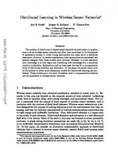
Figure 1: Two lists of candidate target types for a T 80 tank from two SAR sensors. Figure 1 illustrates two lists of candidate target types for a T 80 tank from two SAR sensors. One of the SAR sensors confuses the T 80 tank with an M 1A1 tank in list (b). Hence, the low quality sensor data
cannot be used directly for high-level plans and has to be delivered to other nodes for fusion in the system. If sensor a detects a target TK on the ground, it will generate an event ei about target TK . Formally, an event ei about target TK can be denoted as a tuple hsender, identity, location, timestamp, T T L, pedigreei, where • sender is the ID of the sensor that detects the target. In practice, the ID could be a random number chosen in a range large enough so that any two sensors will have different IDs. 1 • identity is the decision about the target from the sensor. In our approach, it refers to a multiple hypotheses decision from SAR sensors. • location is the location of the target TK being detected, denoted as hxK , yK , zK i. • timestamp is the time that the target is detected by the sensor. The location and timestamp of a target are mainly used in the data association process to determine if two events are referring to the same target. 2 • TTL (time-to-live) is the maximal number of hops allowed for the event propagation in the sensor system. • pedigree is the list of nodes event ei has visited, denoted as L. Note that pedigree is used to avoid cycles during event propagation.
a
ei
d
ej
b
e
ej
ek
ei
c
Figure 2: An example of data flows in the sensor system, where ei , ej , and ek are three relevant events from sensors a, d, and e and all of them refer to target TK . The process of sensor data delivery can be briefly described as follows. When sensor a receives or generates an event ei about TK , it first tries to fuse ei with its previous events about target TK using data fusion techniques such as Dempster-Shafer theory. If the confidence of fused events meets a threshold, sensor node a will stop the propagation of event ei and become a sink node for relevant events of TK . Otherwise, sensor a will choose 1 One advantage of random numbers is that they scale well to large numbers of autonomous sensors which may dynamically enter and leave the sensor system. 2 The discussion of distributed data association in sensor systems is outside of the scope of this paper. Readers may refer to [18, 19] for more information.
one of its neighbors to continue the delivery unless its TTL is zero. Figure 2 shows an example of data flows in the system. The solid lines correspond to directed communication channels between sensor nodes. The arrows in dashed lines represent information flows of relevant events ei , ej , and ej for target TK . As shown in Figure 2, the three events are fused at node c.
3
Adaptive Decision Fusion
Commonly used frameworks for multiple hypothesis decision fusion are Bayesian inference method and Dempster-Shafer theory. Dempster-Shafer theory produces identical results as Bayesian inference method for multisensor decision fusion when the hypotheses about individual target’s identity declarations are singletons and mutually exclusive [20, 21, 22]. However, Bayesian inference method cannot apply to decision fusion in our scenario, as most tactical sensors are incapable of assigning all confidences to each target type. For example, in Figure 1, the nonzero confidence assigned to CLUTTER is not mutually exclusive with other target types. On the contrary, Dempster-Shafer theory allows confidences to be assigned to sets of propositions rather than to just N mutually exclusion propositions. Therefore, we choose Dempster-Shafer theory as our underlying reasoning framework for decision fusion.
3.1
Dempster-Shafer theory
We now introduce the key concepts of the DempsterShafer theory. Let V = {v1 , v2 , . . . , vn } be the set of possible vehicle types, where vi , 1 ≤ i ≤ n, is the possible type of vehicles a SAR sensor can recognize. In practice, a SAR sensor will report confidence levels for around three dozen entities. The SAR sensor we simulate will report confidence levels for a dozen entities (see Figure 1). A frame of discernment Θ = {v1 , v2 , . . . , vn } is the set of hypotheses under consideration and vi ∈ V . Definition 1 Let Θ be a frame of discernment. A basic probability assignment (bpa) is aP function m : 2Θ 7→ ˆ = 1. [0, 1] where (1) m(φ) = 0, and (2) A⊂Θ m(A) ˆ In this paper we consider a common frame of discernment for all SAR sensor outputs. The frame of discernment Θ is {T 80, T 72M, M 1, M 1A1, M 1A2, 2S6, ZSU 23, M 977, M 35, AV EN GER, HM M W V, SA9}. In our scenario, the basic probability assignment can be defined as follows: (1) for any target type vi ∈ V , m({vi }) = c(vi ), where c(vi ) is the confidence level of vi in the table; (2) for any Aˆ ⊆ Θ and Aˆ ∈ / V, ˆ = 0; (3) m(Θ) = c(CLU T T ER), where we m(A) assign the confidence of CLUTTER to the set of all possible target types. ˆ is For a subset Aˆ of Θ, the belief function Bel(A) defined as the sum of the beliefs committed to the posˆ For individual members of Θ, Bel and sibilities in A. m are equal. Thus
Bel({T 80}) = m({T 80}) Bel({T 72M }) = m({T 72M }) A subset Aˆ of a frame Θ is called a focal element of ˆ > 0. Given two a belief function Bel over Θ if m(A) belief functions over the same frame of discernment but based on distinct bodies of evidence, Dempster’s rule of combination enables us to compute a new belief function based on the combined evidence. For every ˆ to subset Aˆ of Θ, Dempster’s rule defines m1 ⊕ m2 (A) be the sum of all products of the form m1 (X)m2 (Y ), where X and Y run over all subsets whose intersection ˆ is A. Definition 2 (Dempster’s rule of combination) Let Bel1 and Bel2 be belief functions over Θ, with basic probability assignments m1 and m2 , and focal elements Aˆ1 , . . . , Aˆk , and Bˆ1 , . . . , Bˆl , respectively. Suppose P ˆ ˆ i,j,Aˆi ∩Bˆj =φ m1 (Ai )m2 (Bj ) < 1 Then the function m : 2Θ 7→ [0, 1] that is defined by m(φ) = 0, and P ˆ = m(A)
ˆ i,j,Aˆi ∩Bˆj =A
1−
P
m1 (Aˆi )m2 (Bˆj ) m1 (Aˆi )m2 (Bˆj )
(1)
i,j,Aˆi ∩Bˆj =φ
for all non-empty Aˆ ⊂ Θ is a basic probability assignment [23]. Bel, the belief function given by m, is called the orthogonal sum of Bel1 and Bel2 . It is written as Bel = Bel1 ⊕ Bel2 . Note that Dempster’s rule of combination is associative and commutative. This means that the processes of combining evidence from multiple sensors are independent of the order in which the sensor outputs are combined. For any vi ∈ V , m({vi }) can be simplified as m1 ({vi })m2 ({vi }) + m1 ({vi })m2 (Θ) + m2 ({vi })m1 (Θ) P 1 − vj ∈V m1 ({vj })(1 − m2 ({vj }) − m2 (Θ)) (2) Similarly, we can compute m(Θ) as m1 (Θ)m2 (Θ) m ({v 1 j })(1 − m2 ({vj }) − m2 (Θ)) vj ∈V (3) When a sensor fuses the data from multiple sensors, it needs to determine if it should stop the data propagation. The key challenge here is how to derive the confidence for a target from the fused sensor data. Next we define a rule which works for the SAR sensor data in our scenario. m(Θ) =
1−
P
Definition 3 Let m be the basic probability assignment for the fused sensor data of target TK , the confidence of TK is defined as C(TK ) = maxvi ∈V m({vi }) + m(Θ)
(4)
USSR T80 USSR T72M US M1 US M1A1 US M1A2 USSR 2S6 USSR ZSU23 US M977 US M35 US AVENGER US HMMWV USSR SA9 CLUTTER
0.4 0.3 0.05 0.05 0.05 0.02 0.03 0.001 0.001 0.001 0.001 0.001 0.095
(a)
USSR T80 USSR T72M US M1 US M1A1 US M1A2 USSR 2S6 USSR ZSU23 US M977 US M35 US AVENGER US HMMWV USSR SA9 CLUTTER
0.05 0.05 0.20 0.28 0.27 0.02 0.03 0.001 0.001 0.001 0.001 0.001 0.105
USSR T80 USSR T72M US M1 US M1A1 US M1A2 USSR 2S6 USSR ZSU23 US M977 US M35 US AVENGER US HMMWV USSR SA9 CLUTTER
0.25 0.19 0.13 0.17 0.17 0.02 0.03 0.0 0.0 0.0 0.0 0.0 0.04
(b)
Figure 3: The fused confidence levels for for a ground target T 80 tank using Dempster-Shafer theory. Figure (a) and (b) show the two SAR sensor reports and the belief function for the fused sensor reports. Figure 3 shows an example of fused confidence levels for a ground target T 80 tank. The confidence of the T 80 tank is m({T 80}) + m(Θ) = 0.29. Note that, the value of C(TK ) is different from c(vi ), where C(TK ) refers to the plausibility to a target type and c(vi ) is the support to the target type vi . For the same (fused) sensor report, we have C(TK ) ≥ c(vi ) when vi is the target type with highest confidence level. Moreover, we can see the value of C(TK ) does not increase monotonically in the fusion process as the sensor reports sometimes provide conflicting evidence defined on the same frame of discernment. In Figure 3, we can find that the first sensor recognizes the true identity of the target (Figure 3 (a)), while the second one misclassifies it as an M 1A1 tank (Figure 3 (b)). Definition 4 Given a set of sensor reports from sensors {s1 , . . . , sL }, the combined belief for fused sensor reports can be denoted as m = m1 ⊕ . . . ⊕ mL
(5)
where ⊕ is the operator in Dempster’s rule of combination. Given a threshold level, e.g., ω, a sensor will determine the number of sensor reports that needs to be fused. The number is dynamically changing and adaptive to the threshold level and the specific type of the ground target. For example, it may need four sensor reports for a T 80 tank, but for a military truck HMMWV, it will require seven or eight sensor reports. The following definition describes the rule for adaptive decision fusion in a distributed sensor system. Definition 5 For any incoming event ei for target TK , a sensor will stop the propagation of ei if and only if the confidence of fused sensor data (including ei ) is greater than the threshold ω, denoted as C(TK ) > ω. Once a sensor finds the confidence of target TK is above the given threshold ω, the sensor will pass the information to the team coordination layer of the sensor system. Specifically, it will create an information token about target TK when it successfully fused the relevant sensor data for target TK with high confidence,
e.g., C(TK ) > ω. Information tokens are then used for high-level team coordination such as task and resource allocation [5]. For example, the system will autonomously allocate the task of attacking the target to a nearby UAV that possesses the required type of munitions.
3.2
Weighted Majority Algorithm
In Section 3.1, we provide a theoretical framework for uncertain sensor data fusion using Dempster-Shafer theory. In practice, the data from different sensors may not be equally reliable due to sensor malfunction or severe weather conditions. Therefore, it is important to take this into consideration during the fusion process and qualify the performance degradation of fusion results. Next we introduce the weighted majority algorithm (WMA) and its variant continuous weight majority algorithm (WMC). We also provide a novel learning algorithm for determining the quality of sensor data in the fusion process. The weighted majority algorithm (WMA) deals with how to make an improving series of predictions based on a set of advisors [16]. The first idea is to assign weights to the advisors, e.g., wi , and to make a prediction based on the weighted sum of the ratings provided by them. The second idea is to tune the weights after an unsuccessful prediction so that the relative weight assigned to the successful advisors is increased and the relative weight assigned to the unsuccessful advisors is decreased. WMA aims to design a master algorithm that applies to the combination of evidence without regard to the reasoning on which the individual ratings might be based. To motivate our approach, we describe a variant of WMA called WMA Continuous (WMC) [16]. WMC allows the predictions of the algorithms to be chosen from the interval [0, 1], instead of being binary. The term trial refers to an update step. We assume that the master algorithm is applied to a pool of n algorithms, letting xji denote the prediction of the ith algorithm of the pool in trial j. Let λj denote the prediction of the
master algorithm in trial j, ρj denote the result of trial j and w1j , . . . , wnj denote the weights at the beginning (j+1) (j+1) of trial j. Consequently, w1 , . . . , wn denote the weights after the trial j. All initial weights wi1 are positive. Let sj =
Pn i=1
wij .
Prediction: The prediction of the master algorithm is Pn j j w x λj = i=1sj i i Update: For each algorithm in the pool, the weight wij is multiplied by a factor θ that depends on β, xji , and ρj . (j+1)
wi
= θwij
where m0 is the weighted average of belief functions . . . m0L and m0i is the updated belief function, 1 ≤ i ≤ L. Note that, when we consider the quality of sensor data in the fusion process, the confidence for target TK needs to be revised as m01
C(TK ) = maxvi ∈V m0 ({vi }) + m0 (Θ).
where θ can be any factor that satisfies j
The weight scheme can effectively mitigate the conflict between evidences, as two sensors will not be P trusted equally anymore. Note that we use L wi / i=1 wi instead of wi to adjust the sensor data, where 0 ≤ wi ≤ 1. 3 Similarly, we can give the prediction and updating rules for the reliability of each sensor during the process of decision fusion. Prediction: The total belief of sensor s for target TK is m0 = m01 ⊕ . . . ⊕ m0L (6)
Update: The weight of sensor si will be updated as follows.
j
β |xi −ρ | ≤ θ ≤ 1 − (1 − β)|xji − ρj | and 0 < β < 1.
3.3
wi0 = θwi
Quality of Information
We adapt the algorithm to predict the reliability of a given sensor based on a set of reports from the sensor. Each fusion node maintains a weight wi for each of the other sensors whose reports need to be fused. This weight estimates how reliable the given sensor is. However, applying the classical WMA for sensor systems presents a technical challenge, because sensor reports are not scalars, but rather belief functions. Therefore, our approach extends WMA to accommodate belief functions. Basically, our approach computes the difference between a prediction of fused sensor reports and each sensor report using the notion of conflict in Dempster-Shafer theory and accordingly updates the weight for each sensor. Suppose sensor s wishes to evaluate the confidence of fused sensor reports from sensors {s1 , . . . , sL }. The assumption here is that we should trust the majority of sensor outputs. Let s assign a weight wi to sensor si . The weight wi is initialized to 1 if s gets the data from si for the first time. Definition 6 Given a sensor si ’s probability mass function mi , its corresponding reliability factor (or weight) wi , the updated belief function can be defined as 0
mi (A) = wi mi (A)/
L X
wi
i=1
0
(7)
mi (Θ) = wi mi (Θ)/
L X i=1
where A ⊂ Θ and A 6= Θ .
wi + 1 − wi /
L X i=1
wi
In weighted majority algorithm, θ can be any value chosen between β ρ and 1 − (1 − β)ρ. For simplicity, we choose the upper bound as the value of θ. θ = 1 − (1 − β)φ.
(8)
Here φ is the conflict between the prediction of fused sensor data and each sensor report in Dempster-Shafer theory. For a given sensor report from sensor si , φ is defined as φ=
X
m0 ({vj })(1 − mi ({vj }) − mi (Θ))
(9)
vj ∈V
where vj is defined as maxvj ∈V m0 ({vj }) and m0 is the basic probability assignment for the fused sensor data. The above formula can be simplified as follows if β = 0.5. θ =1−
φ 2
(10)
Equation 10 indicates that the value of θ relies on the conflict between the prediction m0 and a sensor report. If the conflict φ is large, θ will be small. Correspondingly, the weight of the sensor is reduced to a low level. Algorithm 1 describes the learning algorithm used by each sensor to adjust the weights of other sensors during the fusion process. We can find that the effect of the sensor is minimized in the fusion process when it returns unreliable sensor reports. 3 According to [24], the use of quality of information for decision fusion also solves the limitation of Dempster’s rule of combination for two totally conflicting events.
s1 USSR T80 USSR T72M US M1 US M1A1 US M1A2 USSR 2S6 USSR ZSU23 US M977 US M35 US AVENGER US HMMWV USSR SA9 CLUTTER
0.4 0.3 0.05 0.05 0.05 0.02 0.03 0.001 0.001 0.001 0.001 0.001 0.095
s2 0.05 0.05 0.20 0.28 0.27 0.02 0.03 0.001 0.001 0.001 0.001 0.001 0.095
Target #1 s3 s4 0.4 0.3 0.05 0.05 0.05 0.02 0.03 0.001 0.001 0.001 0.001 0.001 0.095
s5
0.3 0.4 0.05 0.05 0.05 0.02 0.03 0.001 0.001 0.001 0.001 0.001 0.095
0.4 0.3 0.05 0.05 0.05 0.02 0.03 0.001 0.001 0.001 0.001 0.001 0.095
s1
s2
0.3 0.4 0.05 0.05 0.05 0.02 0.03 0.001 0.001 0.001 0.001 0.001 0.095
0.4 0.3 0.05 0.05 0.05 0.02 0.03 0.001 0.001 0.001 0.001 0.001 0.095
Target #2 s3 s4 0.4 0.3 0.05 0.05 0.05 0.02 0.03 0.001 0.001 0.001 0.001 0.001 0.095
0.05 0.05 0.20 0.28 0.27 0.02 0.03 0.001 0.001 0.001 0.001 0.001 0.095
s5 0.4 0.3 0.05 0.05 0.05 0.02 0.03 0.001 0.001 0.001 0.001 0.001 0.095
Figure 4: The sensor outputs for two ground targets T80 tanks, #1 and #2. Here we consider five sensors s1 , . . . , s5 and each column in the figure refers to the decision from a SAR sensor.
4
Experiments
In this section, we first introduce a modeling and simulation environment, OTBSAF (OneSAF Testbed Baseline) 4 [25]. And then we show a simple example of adaptive decision fusion rules and the learning algorithm for quality of information.
4.1
OTBSAF System
OTBSAF models common military vehicles, aircraft, and sensors, and simulates uncertainty for entities’ individual and doctrinal behaviors in the battlefield. We extend OTBSAF and integrate it with our RETSINA multiagent system. One of our contributions to OTBSAF is to add three simulated mounted sensors, SARSim, EOSim, and GMTISim, to the simulation environment. The SARSim simulates an automatic target recognition (ATR) system that receives its input from a synthetic aperture radar (SAR) that is operating in spotlight-mode. In spotlight-mode, a SAR scans an area of terrain, and the ATR will attempt to recognize any stationary object within the bounds of that scanned area. The output from the SARSim is a list of candidate target types (e.g., M1 tank, T80 4 http://www.onesaf.org/
Tank, etc.) with different confidence levels. While a real SAR/ATR system will report confidence levels for around three dozen entities, SARSim will report for a dozen entities. The GMTISim simulates a ground moving target indicator (GMTI) radar, which focuses a radar beam on one spot, and if it detects a moving target there with its ATR system, a motion tracker mechanism follows the movement of the target. While very similar in output and behavior to the SARSim, it is complementary, because it only recognizes entities that are moving, while the SARSim only recognizes entities that are stationary. The EOSim simulates an electro-optical sensor that detects targets at distances and in conditions in which they would be detectable in the ultraviolet, visible, and infrared light spectra. Here we only consider the sensor data from SARSim. We assume there are multiple T 80 tanks on the ground and a team of UAVs are scheduled to scan the area.
4.2
Adaptive Decision Fusion
In the first example, we study the dynamics of the confidence for two T 80 tanks for a series of sensor reports from sensors {s1 , s2 , . . . , s5 }. 0.7 0.6 0.5 Confidence
Algorithm 1 Learning the quality of sensor data by sensor s 1: Initialize sensor si ’s weight to 1 if si returns the data to sensor s for the first time 2: Let {s1 , . . . , sL } be the sensors which return reports to sensor s for target TK 3: Sensor s generates a prediction as specified in Equation 6 4: for each sensor si do 5: Sensor s computes the prediction from the report of si 6: Sensor s updates the weight wi according to Equation 8 7: end for
0.4 0.3 0.2 0.1 0 1
2
3
4
5
Number of reports Target #1
Target #2
Figure 5: An example of the dynamics of the fused sensor data confidence for two T 80 tanks.
Figure 5 shows the confidence for two targets #1 and #2 on the ground, where X-axis shows the the number of sensor reports fused to get the confidence, Y-axis describes the confidence of fused reports. We can find that, for both targets, their confidence levels do not increase monotonically. For example, the confidence of target #1 drops from 0.49 to 0.28 after fusing the first two sensor reports. The reason is that the data from sensor s2 misclassifies the target as an M 1A1 tank. Moreover, the confidence levels for both targets reach a relatively high level. If we set the threshold ω as 0.6, the sensor s which fuses these sensor reports can now recognize the type of target and initialize of a plan if necessary.
4.3
Learning the Quality of Sensor Data
In the second example, we illustrate the change of sensor reliability during the fusion process. Here we assume that sensor s receives the reports for target #1 and #2 from the same set of sensors.
5
Conclusions
In this paper we present a novel approach to reasoning about uncertain and noisy sensor data in distributed autonomous sensor systems. We incorporate data reliability into uncertain sensor data modeling within the framework of Dempster-Shafer theory, where each sensor learns reliabilities of other sensors using a novel application of the weighted majority algorithm. One drawback of our approach is that it is based on a degree of consensus among various sensor sources. This may not work occasionally when the majority of sensors are unreliable and they provide conflicting evidence. In future work, we plan to explore the limitations of our approach. One way to address this drawback is to introduce some context information into the system, such as the expert knowledge in the sensor systems domain [26, 27]. We also would like to investigate the effectiveness of our approach with large amounts of sensor data from various sensors and its effects on high-level information fusion, such as force structure recognition and intent inference [28, 29].
Acknowledgments 1.2
The authors would like to thank Joseph Giampapa, Sean Owens, Robin Glinton, Young-Woo Seo, Charles Grindle, and Dr. Michael Lewis for their contribution to the system development and their helpful comments. The authors would also like to thank our partners at Northrop-Grumman for their assistance in developing some of the external sensor simulators. This research was supported by AFOSR under grants F49640-01-10542. and by AFRL/MNK grant No. F08630-03-10005.
Sensor Reliability
1 0.8 0.6 0.4 0.2 0 1 Sensor s1
Sensor s2
2 Sensor s3
3 Sensor s4
Sensor s5
Figure 6: The sensor reliability after one and two rounds of sensor reports. As we discussed in Section 3.3, we use a weight to denote the reliability of each sensor in the fusion process. The weight is initialized as one and updated according to the weighted majority algorithm. Figure 6 shows the sensor reliability after sensor s receives the two rounds of sensor reports, one for target #1 and another for target #2 when β = 0.5. From Figure 6 we can see that sensor s2 returns low quality of sensor data. Consequently, sensor s decreases its reliability (or weight w2 ), so the effect of low quality data is minimized in the fusion process. Also, in the WMC version of weighted majority algorithm, the weight for each sensor wi may keep decreasing, since there is always a non-zero conflict between a single sensor report and the fused sensor data. In order P to avoid this problem, we use wi / P wi instead of wi in the fused process. P Note that wi / wi may be greater than wi when wi < 1.
References [1] Chee-Yee Chong and Srikanta P. Kumar. Sensor networks: Evolution, opportunities, and challenges. Proceedings of the IEEE, 91(8):1247–1256, 2003. [2] Deborah Estrin, Ramesh Govindan amd John Heidemann, and Satish Kumar. Next century challenges: Scalable coordination in sensor networks. In MobiCom, pages 263–270, 1999. [3] Victor Lesser, Charles Ortiz, and Miland Tambe, editors. Distributed Sensor Networks: A Multiagent Perspective. Kluwer Academic Publishers, 2003. [4] Feng Zhao and Leonidas Guibas. Wireless Sensor Networks: An Information Processing Approach. Morgan Kaufmann Publishers, 2004. [5] Paul Scerri, Yang Xu, Elizabeth Liao, Justin Lai, and Katia Sycara. Scaling teamwork to very large teams. In AAMAS, pages 888–895, 2004.
[6] Robin R. Murphy. National science foundation summer field institute for rescue robots for research and response. AI Magazine, 25(2):133–136, 2004.
[19] James Manyika and Hugh Durrant-Whyte. Data Fusion and Sensor Management: A Decentralized Information-Theoretic Approach. Ellis Horwood, 1994.
[7] H. Van Dyke Parunak, Sven A. Brueckner, and James J. Odell. Swarming coordination of multiple UAV’s for collaborative sensing. In Proceedings of the Second AIAA Unmanned Unlimited Systems Technologies and Operations Aerospace Land and Sea Conference and Workshop, 2003.
[20] Authur P. Dempster. A generalization of bayesian inference. Journal of the Royal Statistical Society, 1968.
[8] Milind Tambe. Towards flexible teamwork. Journal of Artificial Intelligence Research, 7:83–124, 1997. [9] David L. Hall and James Llinas. An introduction to multisensor data fusion. In Proceedings of the IEEE, pages 6–23, 1997. [10] David L. Hall and Sonya A. H. McMullen. Mathematical Techniques in Multisensor Data Fusion. Artech House Publishers, second edition, 2004. [11] Zeineddine Chair and Pramod K. Varshney. Optimal data fusion in multiple sensor detection systems. IEEE Transactions on Aerospace and Electronic Systems, 22(1):98–101, 1986. [12] Stelios C.A. Thomopoulos, R. Viswanathan, and D. C. Bougoulias. Optimal decision fusion in multiple sensor systems. IEEE Transactions on Aerospace and Electronic Systems, 23(5):644–653, 1987. [13] Stelios C.A. Thomopoulos. Theories in distributed decision fusion: Comparison and generalization. In Proceedings of the SPIE, pages 623– 634, 1991. [14] Ruixin Niu, Pramod K. Varshney, M. Moore, and Dale Klamer. Decision fusion in a wireless sensor network with a large number of sensors. In Proceedings of the Seventh International Conference on Information Fusion, 2004. [15] Galina L. Rogova and Vincent Nimier. Reliability in information fusion: Literature survey. In Proceedings of the Seventh International Conference on Information Fusion, pages 1158–1165, 2004. [16] Nick Littlestone and Manfred K. Warmuth. The weighted majority algorithm. Information and Computation, 108(2):212–261, 1994. [17] Allison Ryan, Marco Zennaro, Adam Howell, Raja Sengupta, and J. Karl Hedrick. An overview of emerging results in cooperative UAV control. In Proceedings of 43rd IEEE Conference on Decision and Control, 2004. [18] Erik Blasch and Lang Hong. Data association through fusion of target track and identification sets. In Proceedings of the Third International Conference on Information Fusion, 2000.
[21] John J. Sudano. Equivalence between belief theories and naive bayesian fusion for systems with independent evidential data: Part I, the theory. In Proceedings of the Sixth International Conference on Information Fusion, pages 1239–1243, 2003. [22] John J. Sudano. Equivalence between belief theories and naive bayesian fusion for systems with independent evidential data: Part II, the example. In Proceedings of the Sixth International Conference on Information Fusion, pages 1357–1364, 2003. [23] Glenn Shafer. A Mathematical Theory of Evidence. Princeton University Press, Princeton, NJ, 1976. [24] Rolf Haenni. Shedding new light on Zadeh’s criticism of dempster’s rule of combination. In Proceedings of the Eighth International Conference on Information Fusion, 2005. [25] Joe Giampapa, Katia Sycara, Sean Owens, Robin Glinton, Young-Woo Seo, Bin Yu, Charles E. Grindle, Yang Xu, and Michael Lewis. An agentbased C4ISR testbed. In Proceedings of the Eighth International Conference on Information Fusion, 2005. [26] Subrata Das and David Lawless. Trustworthy situation assessment via belief networks. In Proceedings of the Fifth International Conference on Information Fusion, pages 543–549, 2002. [27] Subrata Das and David Lawless. Truth maintenance system with probabilistic constraints for enhanced level two fusion. In Proceedings of the Eighth International Conference on Information Fusion, 2005. [28] Robin Glinton, Joe Giampapa, Sean Owens, Katia Sycara, Charles Grindle, and Mike Lewis. Intent inferencing using an artificial potential field model of environmental influences. In Proceedings of the Eighth International Conference on Information Fusion, 2005. [29] Bin Yu, Joe Giampapa, Sean Owens, and Katia Sycara. An evidential model of multisensor decision fusion for force aggregation and classification. In Proceedings of the Eighth International Conference on Information Fusion, 2005.