Progress In Electromagnetics Research M, Vol. 37, 175–182, 2014
A Fast EPILE+FBSA Method Combined with Adaptive Cross Approximation for the Scattering from a Target above a Large Ocean-Like Surface Gildas Kubick´ e1, * , Christophe Bourlier2 , Sami Bellez2 , and Hongkun Li2
Abstract—The rigorous evaluation of the NRCS (Normalized Radar Cross Section) of an object above a one-dimensional sea surface (2D case) needs to numerically solve a set of discretized integral equations involving a large number of unknowns. Thus, the direct solution of the impedance matrix equation via LU decomposition becomes the most expensive step in the MoM (Method of Moments) procedure. So, in order to minimize the computation cost, the iterative domain decomposition method called EPILE (Extended Propagation-Inside-Layer Expansion) was used and then was combined with the FBSA (Forward-Backward with Spectral Acceleration) to calculate the local interactions on the rough sea surface. The resulting fast method is called EPILE+FBSA. In this paper, we take advantage of the rank-deficient nature of the coupling matrices, corresponding to the object-surface interactions, to further reduce the complexity of the method by using the ACA (Adaptive Cross Approximation). Thus, the coupling matrices are strongly compressed without a loss of accuracy and the memory requirement is then strongly reduced. For a cylinder above a rough sea surface, the results show the efficiency of the accelerated EPILE+FBSA+ACA method.
1. INTRODUCTION The study of scattering from an object above a rough surface is a subject of great interest. The applications of such research concern many areas such as remote sensing, radar surveillance, optics and acoustics. Here, we focus on the scattering from an object above a random rough sea surface. A way to solve rigorously this scattering problem is to use the well-known Method of Moments (MoM) [1]. Nevertheless, since the number of unknowns is huge, a brute force MoM (direct LU inversion of the impedance matrix) cannot be applied and then accelerations are needed to reduce the memory requirement and the computing time. For a 2D scattering problem (problem geometry invariant with respect to one direction), a review is presented in [2]. Then, the EPILE (Extended Propagation-InsideLayer Expansion) method based on a domain decomposition, is a good candidate for iteratively solving the MoM impedance matrix equation. Initially, this method was developed to the scattering from a stack of two one-dimensional interfaces (the upper surface is only illuminated) separating homogeneous media [3] and, was generalized to the case of two illuminated scatterers [4, 5]. The main advantage of EPILE is that it avoids the direct solution of the whole MoM matrix equation by using the partitioned inverse matrix formulas and an iterative scheme. The two first steps are dedicated to handling the initial current densities and two other steps, repeated in an iterative process, to account for the current densities due to the coupling interactions between the two scatterers. Furthermore, the EPILE method was accelerated by combining it with FBSA (Forward-Backward Spectral-Acceleration which is valid for Received 25 May 2014, Accepted 22 July 2014, Scheduled 30 July 2014 * Corresponding author: Gildas Kubick´ e (
[email protected]). 1 DGA/DT/MI (Direction G´ en´ erale de l’Armement — Direction Technique — Maˆıtrise de l’Information), CGN1 Division, France. 2 IETR (Institut d’Electronique et des T´ el´ ecommunications de Rennes) Laboratory, LUNAM Universit´ e, Universit´ e de Nantes, France.
176
Kubick´ e et al.
a single surface) [6] for the computation of the local interactions (which evaluate the current density) on the rough surface (sampled into N2 points), whereas the current density on the object (sampled into N1 points) were computed from a direct LU inversion [4]. The complexity of the resulting method, EPILE+FBSA, is then related to the calculations of the: • Local interactions on the object (from a direct LU inversion): O(N13 ) multiplications and O(N12 ) terms for the memory requirements. • Local interactions on the surface (from FBSA): O(PFB N2 Ns ) multiplications and O(N2 Ns ) terms for the memory requirements, in which PFB is the order of the iterative scheme of the ForwardBackward method and Ns is the integer part of xds /∆x2 ; xds being the strong interaction distance for the Spectral Acceleration and ∆x2 the sampling step on the rough surface. • Matrix-vector products for the coupling steps: O(N2 N1 ) multiplications and O(N2 N1 ) terms for the memory requirements. Since the number of unknowns on the rough surface is much greater than that on the object, the acceleration was focused on the computation of the current density on the rough surface. Then, one of the most expensive step (in computing time and memory requirements) is related to the matrix-vector products in the coupling steps. One can notice that the coupling matrices are rank-deficient since only well-separated MoM interactions are involved. Thus, in order to accelerate the matrix-vector products involved in the coupling steps, a recent algebraic method called Adaptive Cross Approximation (ACA) is applied to compress the coupling matrices. This method, developed in 2000 by Bebendorf [7, 8], was then applied to electromagnetics [9–13] and can be seen as a truncated and partially pivoted Gaussian elimination [7]. In this paper, the ACA method is hybridized with EPILE+FBSA, permitting to solve a problem with a huge number of unknowns thanks to a much smaller storage requirement and computing time than those from a direct LU inversion. The bistatic NRCS is computed for a wide frequency band (from f = 2 GHz to f = 20 GHz). To describe the sea surface height (its distribution is assumed to be Gaussian), the Elfouhaily et al. [14] roughness spectrum is applied. It was shown in [2] that to include all the surface roughnesses, the minimum surface length must satisfy Lmin ≈ 1.6u210 where Lmin is expressed in meters and u10 in m/s. Then, by considering a sampling step of λ0 /10 and u10 = 10 m/s at f = 15 GHz (λ0 = 2 cm), N2 = 80, 000 and N1 ≈ 1600 (cylinder of radius of 0.5 m). In addition, since the incident Thorsos [15] tapered wave is used to reduce the edges effect, the surface length must be multiplied approximately by 2 in order to take into account the whole statistics of the roughness, and then N2 = 160, 000. This realistic maritime scenario can be simulated from EPILE+FBSA+ACA on a standard personal computer. The paper is organized as follows. The hybridization of EPILE+FBSA with ACA is presented in Section 2. A brief summary of EPILE+FBSA is addressed, then the ACA is applied to compress the coupling matrices for accelerating the coupling steps of EPILE. Section 3 presents results of the NRCS and the last section gives concluding remarks. 2. HYBRIDIZATION OF ACA WITH EPILE+FBSA 2.1. EPILE Combined with FBSA Let us consider two scatterers (with homogeneous media): for example an object (first scatterer) and a rough surface (second scatterer), embedded in an homogeneous medium and illuminated by an incident wave (see Figure 1). The use of the integral equations discretized by the MoM leads to the linear ¯ = b, in which Z ¯ is the impedance matrix of the scene made up of the two scatterers, system ZX b is the incident field, and X is the current density on both scatterers (the field and/or its normal derivative on the surfaces). The EPILE method was developed in order to solve such a linear system efficiently and rigorously. Indeed, by inverting by block the impedance matrix, it can be shown after some mathematical manipulations that the current X1 on the surface S1 of the scatterer 1 is [3–5] X1 =
p=P EPILE X p=0
(p)
Y1 ,
(1)
Progress In Electromagnetics Research M, Vol. 37, 2014
177
Cylinder
θi
(εr0, Ω0)
θs
(εr1, Ω1) S1
S2
z1 >0
x1 (εr2, Ω2) Ocean-like surface
Figure 1. Illustration of the problem: scattering by an object above a rough surface. The media {Ω0 , Ω1 , Ω2 } of permittivities {²r0 , ²r1 , ²r2 } are assumed to be homogeneous, and the scatterers geometries are invariant along the direction normal to the figure. in which
(
³ ´ (0) ¯ −1 b1 − Z ¯ 21 Z ¯ −1 b2 Y1 = Z for p = 0 1 2 . (p) ¯ c,1 Y(p−1) Y1 = M for p > 0 1
(2)
¯ c,1 being the characteristic matrix of the scene (the two scatterers) defined as M ¯ c,1 = Z ¯ −1 Z ¯ 21 Z ¯ −1 Z ¯ 12 , M 1 2 b1 the incident field illuminating the scatterer 1 (from the transmitter) and b2 the incident field ¯ 1 and Z ¯ 2 are the local impedance sub-matrices illuminating the scatterer 2 (from the transmitter). Z ¯ 12 and Z ¯ 21 are the coupling sub-matrices between of scatterer 1 and scatterer 2, respectively, whereas Z the two scatterers. The mathematical expressions of these matrices can be found in [2]. In Eq. (1), the sum is truncated at the order PEPILE obtained from a convergence criterion. By substituting subscripts {1, 2, 12, 21} for subscripts {2, 1, 21, 12} in Equations (1) and (2), the unknowns X2 on the surface S2 can be found. ¯ −1 accounts for the local interactions on the surface S1 , so Y(0) (zeroth order term) corresponds Z 1 1 to the current on the surface of scatterer 1 when it is illuminated by the direct incident field (b1 ) and ¯ 21 Z ¯ −1 b2 ). Indeed, Z ¯ −1 accounts for the local interactions the direct scattered field by the surface S2 (−Z 2 2 ¯ on the lower surface, and Z21 propagates the field on the surface S2 toward scatterer 1. For the first(1) ¯ c,1 Y(0) , Z ¯ 12 propagates the current on the surface S1 , Y(0) , toward scatterer order term, Y1 = M 1 1 ¯ −1 accounts for the local interactions on S2 , and Z ¯ 21 re-propagates the resulting contribution 2, Z 2 ¯ −1 updates the current values on S1 . Thus the characteristic matrix M ¯ c,1 toward scatterer 1; finally, Z 1 propagates the field between the two scatterers in a back and forth manner. In conclusion, the order PEPILE of EPILE method, corresponds to the number of back and forths between the two scatterers. ¯ = b is Then, one of the advantages of EPILE is that the resolution of the linear system ZX reduced to an iterative scheme, which involves the inverse of the impedance matrix of each scatterer. Consequently, if one of the scatterers is a rough surface, the computation of the local interactions ¯ 2 and computation of the matrix-vector product Z ¯ −1 u, where u is a vector) can be done (inversion of Z 2 by using fast numerical method that already exists for scattering from a single rough surface (without the object). So, the FBSA method [6] was used to accelerate this step [4, 5]. 2.2. EPILE+FBSA Combined with ACA As stated in the introduction of the paper, one of the most expensive step remains the matrix-vector ¯ 12 u and Z ¯ 21 u of complexity O(N1 N2 ) (also for the memory requirement). To reduce this products Z complexity and the memory requirement, the ACA algorithm is applied. ¯ of size M × N by a The outline of the ACA algorithm is to approximate a given dense matrix A ˜ (of size M × N too) obtained from a matrix product: matrix A ˜ =U ¯ V. ¯ A
(3)
¯ and V ¯ are two dense matrices of sizes M × k and k × N , respectively, k being the effective where U ¯ The two matrices U ¯ and V ¯ are constructed by the help of an iterative scheme, rank of the matrix A. which can be seen as a rank-revealing LU decomposition [7, 10], which is stopped when the convergence
178
Kubick´ e et al.
¯ and V, ¯ it is reached for a given tolerance threshold ². It is very important to note that to construct U ¯ is not necessary to calculate all the elements of the matrix A to be compressed (unlike a Singular Value Decomposition, SVD). Then, the resulting memory requirement is (M + N )k instead of M × N . For M = N , the compression is efficient if 2k ¿ N . In addition, the complexity of the matrix-vector product ¯ = U( ¯ Vu) ¯ Au also requires (M + N )k multiplications instead of M N . We define the compression ratio as (M + N )k . (4) τ =1− MN If k ¿ (M, N ), then τ is close to 1 (100% of compression), whereas if τ = 0 (case for which M = N = 2k), the compression is not efficient, and if k = M or k = N then τ < 0 and ACA implies a bigger storage requirement than that without ACA. The resulting complexity of EPILE+FBSA+ACA, for a given iteration of EPILE, is O([2 − τ12 − τ21 ]N1 N2 ) + O(PFB N2 Ns ) + O(N12 ), where τ12 and τ21 are the compression ratio of the coupling ¯ 12 and Z ¯ 21 , respectively. As already discussed in the literature, the compression ratio of matrices Z a coupling matrix (off-diagonal block-block or region-region sub-matrix) increases as the interaction distance increases: the farther the interactions are, the weaker the coupling is and the more efficient the compression from ACA is [12]. Then, ACA is obviously not efficient for (self-) impedance matrices ¯ 11 and Z ¯ 22 . (local interactions computation), like Z A way to solve this issue is to split each surface into sub-regions: the resulting self-impedance matrix can be then expressed into diagonal block matrices (which contain the self-coupling terms) and off-diagonal block-block matrices (which take into account the coupling between each sub-regions of the surface) which can be compressible when the regions are spaced some distance apart [12]. Besides, this can be done in a recursive scheme (each subregion can be split into many subregions to exhibit smaller off-diagonal blocks to compress) with a Multi-Level ACA [13], or also with the formalism of ¯ 11 and Z ¯ 22 since H-matrix theory [16, 17]. This is not applied here for the two impedance matrices Z ¯ Z11 is quite small (for an object of small or moderate size) and applying MLACA or H-matrix theory ¯ 22 , the FBSA is already used which provides a can be more expensive than a direct inversion; and for Z ¯2 low complexity: only O(PFB N2 Ns ) for the computation of the local interactions on S2 (inversion of Z −1 ¯ u, where u is a vector). and computation of the matrix-vector product Z 2 3. NUMERICAL RESULTS Since the sea surface is highly conductive for microwave frequencies, the impedance (or Leontovich) boundary condition (IBC) is applied. The object is assumed to be a perfectly-conducting circular cylinder. The simulation parameters are listed in Table 1 (problem depicted in Figure 1). The origin of the coordinate system is located at the mean surface level (vertical position) and at the center of the sea surface (horizontal position). The choice for all the parameters (EPILE order PEPILE , FB order PFB , strong interaction distance for SA) of EPILE-FBSA was already studied for an object above a rough sea surface [5]: they are reported in Table 1. Figures 2, 3 and 4 plot the CPU time, the compression ratios τ12 and τ21 and the memory requirement versus the frequency f , respectively. The labels in the legends mean: • • • •
“LU”: the NRCS is computed from a direct LU inversion of the impedance matrix. “EPILE+FBSA”: the NRCS is computed from EPILE+FBSA. “EPILE+FBSA+ACA”: the NRCS is computed from EPILE+FBSA+ACA. “No filling matrices” means that the CPU time for the matrix filling is not counted when using EPILE+FBSA+ACA method.
The simulations ran on a workstation HPZ800 (dual processor 2.67 GHz (12-core) with 32 GB RAM) and with the MatLab software. NRCS calculation from a direct LU inversion is stopped when the memory requirement exceeds 12 GB. As the frequency increases, Figure 2 shows that the CPU time increases significantly with LU, whereas with EPILE+FBSA and EPILE+FBSA+ACA it increases slower. In addition, as shown in Figure 3, the compression ratio increases with f . ACA allows to reduce both the CPU time and the
Progress In Electromagnetics Research M, Vol. 37, 2014
179
Table 1. Simulation parameters (problem depicted in Figure 1). The object is a perfectly-conducting circular cylinder of radius 0.5 m and the sea surface obeys the IBC approximation. λ0 is the wavelength and Lc is the correlation length of the sea surface (in meters). Wind speed u10 [m/s] Surface length L2 [m] Frequency f [GHz] Sampling step ∆x2 [λ0 ] Incidence angle θi [o ] Object coordinates (x1 , z1 ) [m] Thorsos wave parameter g [m] Polarization EPILE order PEPILE FB order PFB Strong interaction distance for SA [m] ACA convergence threshold 20
90
LU EPILE+FBSA EPILE+FBSA+ACA No filling matrices
18
Compression ratio [%]
16 14 CPU time [mn]
5 120 [2; 20] 0.1 0 (0, 3) L2 /6 = 20 TE 6 5 0.03Lc = 0.0046u2.04 10 0.001
12 10 8 6 4
88
86
84 Matrix Z
2 0 2
Matrix Z
4
6
8
10 12 14 Frequency [GHz]
16
18
20
Figure 2. CPU time (in minutes) versus the frequency f . The simulation parameters are listed in Table 1.
82 2
4
6
8
10 12 14 Frequency [GHz]
16
18
12 21
20
Figure 3. Compression ratios τ12 and τ21 versus f. The simulation parameters are listed in Table 1.
memory requirement as depicted in Figure 4. This figure clearly shows the difficulty to calculate the NRCS with a direct LU inversion when the frequency increases. ¯ 21 (propagation from the surface to the object) It is important to note that the coupling matrix Z is the sum of two matrices (linear combination of boundary conditions with IBC): one is related to the Neumann boundary condition and the other one is related to Dirichlet boundary condition. Then, the compression is applied on this sum of submatrices. As illustratred on Figure 3, the use of IBC does not reduce the compression ratio since τ21 ≈ τ12 for any frequency. Since the coupling matrices (and the impedance matrices too) are independent of the incident wave, the compressed coupling matrices can be stored and then, it does not need to re-calculate them for different incidence angles θi . Thus, the ACA compression is very interesting for a monostatic configuration involving many incidence angles since the compression from ACA is made only one time,
180
Kubick´ e et al. 1
Memory requrement [GB]
10
0
10
"1
10
LU EPILE+FBSA EPILE+FBSA+ACA
"2
10
2
4
6
8
10 12 14 Frequency [GHz]
16
18
20
Figure 4. Memory requirement versus f . The simulation parameters are listed in Table 1. 5 0
NRCS [dB]
-5 -10 -15 -20 -25
LU EPILE 3+FBSA (0.0085) EPILE 3+FBSA+ACA (0.0091) EPILE -1+FBSA (0.2530)
-30 -35 -40 -90
-75
-60
-45
-30
-15
0
15
30
45
60
75
90
Scattering angle θ [°] s
Figure 5. NRCS versus the scattering angles θs for f = 6 GHz. The simulations parameters are listed in Table 1. PEPILE = −1 refers to the case when the coupling between the object and the surface is ignored. and the matrix-vector products are then accelerated (since compressed coupling matrices are involved) for each incident angle. In Figure 2, for a frequency f = 14 GHz (57,466 unknowns), when the CPU time for the matrix filling is not counted when using EPILE+FBSA+ACA method, the computing time is of the order of 5 minutes. Figure 5 plots the bistatic NRCS versus the scattering angles θs for f = 6 GHz (other parameters are listed in Table 1). In the legend, the first number is the EPILE convergence order PEPILE = 3, obtained when the RRE (Relative Residual Error) is smaller than 0.01. The RRE is defined as ²=
normθs (NRCSMETHOD − NRCSLU ) , normθs (NRCSLU )
(5)
where norm stands for the norm two. It corresponds to the second number in the legend. Figure 6 plots the bistatic NRCS versus the scattering angles θs for f = 6 GHz. Other parameters are listed in Table 1 except θi = 45o , TM polarization, PEPILE = 2 and PFB = 2. Figures 5 and 6 show that the curves perfectly match in cases of both TE and TM polarization, meaning that ² < 0.01 and ²ACA < 0.001 (ACA convergence threshold) are good values. The order PEPILE = −1 corresponds to the case, for which the coupling is not included between the surface and the object (both scatterers are considered as in free space). The comparisons show that the coupling must be accounted for. Figure 7 illustrates this by plotting the NRCS ratio which corresponds to the
Progress In Electromagnetics Research M, Vol. 37, 2014
181
5 LU EPILE 2+FBSA (0.0068) EPILE 2+FBSA+ACA (0.0072) EPILE -1+FBSA (0.3949)
0
NRCS [dB]
-5 -10 -15 -20 -25 -30 -35
-40 -90 -75
-60
-45
-30
-15
0
15
30
45
60
75
90
Scattering angle θ s [°]
Figure 6. NRCS versus the scattering angles θs for f = 6 GHz. The simulations parameters are listed in Table 1 except θi = 45o , TM polarization, PEPILE = 2 and PFB = 2. PEPILE = −1 refers to the case when the coupling between the object and the surface is ignored. 4
NRCS ratio [dB]
3 2 1 0 -1 -2 -3
EPILE 2+FBSA (0.0068) EPILE 2+FBSA+ACA (0.0072) EPILE -1+FBSA (0.3949)
-4 -90 -75
-60
-45
-30
-15
0
15
30
45
60
75
90
Scattering angle θ [°] s
Figure 7. NRCS ratio (with the reference method: direct LU inversion) versus the scattering angles θs for f = 6 GHz. Same parameters as in Figure 6. ratio between the NRCS under test (in linear scale) and the NRCS (in linear scale) of the reference (direct LU inversion) given in dB. One can see that the local error is much stronger without coupling (for PEPILE = −1) than with the coupling of EPILE. Moreover, the impact due to the use of ACA is not very sensitive: the two curves EPILE2+FBSA and EPILE2+FBSA+ACA match well. One can also notice that the ratio with EPILE (with and without ACA) is locally strong when the NRCS is very low while the ratio is very low around the specular direction θs = 45o for which the NRCS is highest. 4. CONCLUSION For an object above a rough surface, the domain decomposition EPILE method has already proven its efficiency by allowing to apply the fast FBSA method to compute the local interactions on the rough sea surface for a large problem, in which two coupled scatterers are involved. In this paper, the EPILE+FBSA method is accelerated by using the ACA thanks to the rank-deficient nature of the coupling matrices involved in EPILE. Indeed, the ACA method permits to strongly compress them without a loss of accuracy and the memory requirement is then strongly reduced. Then, realistic maritime scenario (with a huge number of unknowns) can be simulated from EPILE+FBSA+ACA on a standard personal computer. Finally, the results show the efficiency and accuracy of the proposed method EPILE+FBSA+ACA for a cylinder above an ocean-like surface.
182
Kubick´ e et al.
REFERENCES 1. Harrington, R. F., Field Computation by Moment Method, Macmillan, New York, 1968. 2. Bourlier, C., N. Pinel, and G. Kubick´e, Method of Moments for 2D Scattering Problems. Basic Concepts and Applications, FOCUS SERIES in WAVES, Ed. WILEY-ISTE, 2013. 3. D´echamps, N., N. De Beaucoudrey, C. Bourlier, and S. Toutain, “Fast numerical method for electromagnetic scattering by rough layered interfaces: Propagation-inside-layer expansion method,” Journal of the Optical Society of America A, Vol. 23, No. 2, 359–369, 2006. 4. Kubick´e, G., C. Bourlier, and J. Saillard, “Scattering by an object above a randomly rough surface from a fast numerical method: Extended PILE method combined with FB-SA,” Waves in Random and Complex Media, Vol. 18, No. 3, 495–519, 2008. 5. Kubick´e, G., C. Bourlier, and J. Saillard, “Scattering from canonical objects above a sea-like onedimensional rough surface from a rigorous fast method,” Waves in Random and Complex Media, Vol. 20, No. 1, 156–178, 2010. 6. Chou, H. T. and J. T. Johnson, “A novel acceleration algorithm for the computation of scattering from rough surfaces with the forward-backward method,” Radio Science, Vol. 33, No. 5, 1277–1287, 1998. 7. Bebendorf, M., “Approximation of boundary element matrices,” Numerische Mathematik, Vol. 86, No. 4, 565–589, 2000. 8. Bebendorf, M. and S. Rjasanow, “Adaptive low-rank approximation of collocation matrices,” Computing, Vol. 70, No. 1, 1–24, 2003. 9. Kurz, S., O. Rain, and S. Rjasanow, “The adaptive cross-approximation technique for the 3-D boundary element method,” IEEE Transactions on Magnetics, Vol. 38, No. 2, 421–424, 2002. 10. Zhao, K., M. N. Vouvakis, and J.-F. Lee, “The adaptive cross approximation algorithm for accelerated method of moments computation of EMC problems,” IEEE Transactions on Electromagnetic Compatibility, Vol. 47, No. 4, 763–773, 2005. 11. Shaeffer, J., “LU factorization and solve of low rank electrically large MoM problems for monostatic scattering using the adaptive cross approximation for problem sizes to 1 025 101 unknowns on a PC workstation,” Proc. IEEE Antennas Propag. Soc. Int. Symp., 1273–1276, Sep. 9–15, 2007. 12. Shaeffer, J., “Direct solve of electrically large integral equations for problem sizes to 1M unknowns,” IEEE Transactions on Antennas and Propagation, Vol. 56, No. 8, 2306–2313, 2008. 13. Tamayo, J. M., A. Heldring, and J. M. Rius, “Multilevel adaptive cross approximation (MLACA),” IEEE Transactions on Antennas and Propagation, Vol. 59, No. 12, 4600–4608, 2011. 14. Elfouhaily, T., B. Chapron, K. Katsaros, and D. Vandermark, “A unified directional spectrum for long and short wind-driven waves,” Journal of Geophysical Research, Vol. 102, No. C7, 781–796, 1997. 15. Thorsos, E. I., “The validity of the Kirchhoff approximation for rough surface scattering using a Gaussian roughness spectrum,” Journal of the Acoustical Society of America, No. 83, 78–92, 1988. 16. Hackbusch, W., “A sparse matrix arithmetic based on H-matrices. Part I. Introduction to Hmatrices,” Computing, Vol. 62, No. 2, 89–108, 1999. 17. Grasedyck, L. and W. Hackbusch, “Construction and arithmetics of H-matrices,” Computing, Vol. 70, No. 4, 295–344, 2003.