ON APPLICABILITY OF THE -APPROXIMATION OF THE SURFACE HARMONICS METHOD FOR COMPUTING RBMK-TYPE REACTOR N.I. Laletin, A.A. Kovalishin RRC “Kurchatov Institute” 123182Kurchatov sq., Moscow, Russia
[email protected]
ABSTRACT Results of studies on applicability of some approximations of the Surface Harmonics Methods (SHM) for computing RBMK-type reactors are presented. This paper falls within a series of researches devoted to the analysis of different aspects of the Surface Harmonics Method (SHM) application. This method is aimed at development of computational instruments comparable with referent ones in respect of precision (methodical error is of the order of uncertain information about micro-sections) being at the same time as fast as the existing engineer codes. This paper uses two benchmarks for the cores of RBMK-type reactors in order to show that: 1. The -approximation of the SHM is sufficient for excluding the main part of errors except those connected with cells homogenization, even in case of significant unevenness of neutron fields. 2. Rougher approaches, recently used for calculations of RBMK-type reactors, are very sensitive to the form of field being characterized by significant errors in case of uneven fields. 1.INTRODUCTION Existing mathematical models that describe the behavior of nuclear reactors (including RBMK) imply some artificial adjustment parameters obtained from experiments and tests provided by operating reactors. But such approach seems to be applicable for calculating ordinary situations only being quite unacceptable for computing emergency situations. Indeed, using appropriate 1
correction parameters in the model, we get some interpolation mechanism based on minimization of resulting error with rather broad, but nevertheless, restricted area of application. When trying to simulate emergency situation one cannot be sure that the use of experimental adjustments will result in compensation of errors to the same extent as in calculations of ordinary situations (there simply cannot be sufficient experimental database for emergency situations). The calculation of emergency processes requires a mathematical model free from adjustment parameters. At the same time the accuracy of ordinary situations calculation should be satisfactory for practical purposes. Thus it is necessary to point out all sources of computational error sequentially and then minimize all parts separately but not by compensating errors caused by various factors. The analysis of sources and parts of general computational error in reactor calculations was given in paper1. Following this paper one can point out error items: 1.There is error stipulated by uncertainty regarding knowledge of micro-constants. 2.There are methodical errors that arises during preparation of the group characteristics. 3. There are errors of cell calculations (including homogenization, transition to the diffusion approximation, simplification of power dependence, etc.) 4. There are errors of reactor core calculations. The main goal of presented paper is to study the part of error in calculations of RBMK-type reactors that does not include inaccuracy associated with cell homogenization. We formulate two benchmarks with cores prototyping real RBMK, but with two group sections, obtained as a result of averaging the neutron distribution in cells. The last ones have been received by means of standard calculations, realized by the code WIMS-D4. Hereon, taking characteristics of RBMK cells into consideration, we can take a fine mesh solution in diffusion approximation as a reference one. Then specified problems have been studied using different SHM2,3 approximations. Thus such calculations allow one to value mainly the main mesh size correction and account higher harmonics. Estimation of errors from rough assumptions on cell vicinity and from contribution of nondiagonality of the diffusion coefficient matrixes, appearing in the SHM, is less obtainable. Thus, the same aspects of the SHM as in REF4 for VVER calculations are studied in this paper. However, since features of the VVER and RBMK cores are quite different previous papers do not cover the subject of the current research. As soon as rougher approaches can be applied simultaneously with initial SHM approximations, obtained results can explicitly show inaccuracy of the former.
2
Calculations presented in this paper were made by means of self-developed code SHMQUADRO, but here we provide neither verification, nor validation of this code. The main target here is to study some aspects of the SHM in respect to the RBMK calculations. Note that although RBMK cells were assumed to be homogeneous in this case, the SHM finitedifference equations were obtained without assumption of homogeneous structure of cells and applicability of diffusion approximation. In this work the assumption of homogeneous structure of cells and diffusion approximation are considered within particular case. Such selection of problem is stipulated partly by the intention to separate different parts of total error and partly by the fact that for reactor constructed by homogeneous cells it is possible to obtain exact solution of the diffusion equation. The choice of two-dimensional core instead of three-dimensional one was justified by the problem of big time expenditures when calculating large dimension case and obtaining reference solution. 2.TWO-DIMENSIONAL CALCULATIONS OF THE RBMK CORES The descriptions of two model problems for RBMK and corresponding results obtained in different ways are presented. Description of the finite-difference equations of and approximations of the SHM used in calculations is given in Appendix. Figure 1 shows the map of two RBMK cores. Map for problem N1 corresponds to simplified load of the 4th block of Kursk nuclear power plant as of January 31, 1996. In problem N2 two additional absorbers (AA) were incorporated instead of working channels marked on Figure 1. All cells were considered to be homogeneous. Two-group constants obtained by WIMS for cells of the RBMK were data inputs. The following assumptions have been made for reference solution due to a large dimensionality of the problem: only five types of cells were considered, all fuel cells were supposed to be the same, absorbers of SCP were totally submerged, height buckling Bz2 , matrixes of diffusion coefficients for all types of cells were chosen to be similar. Condition implied zero neutron flux on the external side of reflector was also imposed. Twogroup cell constants are presented in Table I. Table I. Two-group constants for the RBMK test problems.
D1 D2 Σa1 Σa2 Σ1→2 νΣ1 νΣ2
1 1.1017726 0.7998723 0.0011394 0.0041830 0.0044362 0.0006032 0.0057731
2 1.10177267 0.79987234 0.00007333 0.00197129 0.00741269 0.00 0.00
3 1.10177267 0.79987234 0.00077380 0.00470222 0.00639794 0.00 0.00
3
4 1.10177267 0.79987234 0.00287383 0.00472534 0.00406582 0.00 0.00
5 1.10177267 0.79987234 0.00000813 0.00037324 0.00392153 0.00 0.00
3.REFERENCE SOLUTION The fine-mesh solution of two-group diffusion equation was taken as the reference solution. For this purpose calculations with various mesh sizes were made. Equations used for the first and the second groups correspondingly were the following:
4 H2 4 H2
4
D01D 1j
∑D j =1 4
+D
1 j
D02 D 2j
∑D j =1
1 0
2 0
+ D 2j
(Φ
1 0
(Φ
2 0
)
1 2 − Φ1j + ( Σ1a,0 + Σ s 0→ )Φ10 =
)
−Φ + Σ Φ = Σ 2 j
2 a,0
2 0
1→ 2 s0
1 (ν f Σ f 10 Φ10 + ν f Σ f 20Φ20 ) K eff .
(1)
Φ
1 0
.Here H - is a mesh size. When H decreases to zero solutions of equations (1) go to the precise solution of diffusion differential equation. For a problem N1 three calculations with different mesh sizes were carried out, namely H = 4.167 (36 points on a cell), H = 3.125 (64 points on a cell) and H = 2.5 (100 points on a cell). Results of the last calculation were adopted to be the reference. For problem N2 results of calculation with mesh size H = 4.167 (36 points on a cell) were adopted to be the reference. Difference in selection of mesh sizes for various problems will be clear from the analysis of results. 4.RESULTS OF CALCULATIONS In tables 2 and 3 some results of the solution of the test problems obtained by various ways are presented. Table II. Results of calculations of the test problem RBMK N 1
Keff. δKeff. , % Kr δKr. , % Max[dQ], % Max[Q] N{max[Q]} Min[Q] N{min[Q]} %
H=4.167 cm. 0.99088 --------3.071 ----------------3.071 1280 0.223 2272-
H=25.0 cm. 1.02219 3.16 2.722 -11.3 -44.2 2.722 1280 0.211 2272
4
SHM 1.00438 1.36 2.928 -4.7 -19.5 2.928 1280 0.228 2272
SHM 0.99117 0.03 3.072 0.03 3.9 3.072 1280 0.227 2272
Table III. Results of calculations of the test problem RBMK N 2 H=2.5 cm
H=3.125cm.
H=4.167 cm.
H=25.0 cm. SHM 1.02319 1.00675 2.89 1.23 2.819 5.590 -66.0 -32.7 323. 116.5 2.819 5.590 2361 2361 0.159 0.088 190 190
0.99446 Keff. 0.99463 0.99495 -----0.017 0.049 δKeff. , % 8.302 8.281 8.173 Kr -------0.26 -1.55 δKr. , % -------0.3 4.33 max[dQ], % 8.302 8.281 8.173 max[Q] 2361 2361 2361 N{max[Q]} 0.044 0.044 0.046 Min[Q] 190 190 190 N{min[Q]} Denotations in tables II and III: δKeff - deviation of Keff from results of reference calculation; Kr - irregularity coefficient; δKr. - deviation of Kr from results of reference calculation; Max [dQ] - maximum deviation of power density from results of reference calculation; Max [Q] - maximum power density in channel; N {max [Q]} - number of channels with maximum power density; Min [Q] - minimum power density in channel; N {min [Q]} - number of channels with minimum power density;
SHM 0.99535 0.08 8.274 -0.34 2.3 8.274 2361 0.044 190
The columns H = XX designate calculation provided on the scheme (1) with a corresponding mesh size. The columns , correspond to the SHM calculations under approximation of 3 test functions (five-point finite-difference equation) and with 8 test functions (nine-point finitedifference equation). See Appendix for approximate obtaining nine finite-difference equations from the system of equations under -SHM approximation. Note that calculation "H = 25.0 cm." corresponds to codes, broadly used nowadays for RBMK calculations, namely those of BOKR, STEPAN5 type (in their most simplified version). The calculation in this case approximately corresponds to the schemes with corrections of Askew type, etc. The problems N 1 and N 2 differ as one of them (N 2) has rather uniformed fields corresponding to the ordinary condition with factor Kr = 2.7 for calculation with H = 25.0 (calculation under the scheme BOKR). In the second problem field is hardly uneven with Kr = 8.3 for calculation with H = 2.5 cm. This cannot be the case for the ordinary operating reactor but being quite probable for emergency processes. The view of power density distribution for various problems obtained on the various schemes is shown on Figure 25. In the problem with unified field (N1) difference between the most precise solution with H=4.167 cm and that with H=25.0 cm totals 3% in Keff and 11% in irregularity coefficient. However fields of power distribution differ insignificantly in their microstructure (see Figure 4 and 5).
5
5 5 5 5 5 5 5 5 5 5
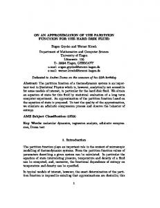
5555555555 55555555555555555555 555555555555555555555555 5555555555555555555555555555 55555555511111111111111555555555 5555555111413141114131411115555555 555555111111111111111111111111555555 55555141114111411141114111411141155555 5555511111111111111111111111111111155555 555551413141314131413141314131413141155555 55555111111111111111111111111111111111155555 5555514111411121114111411141112111411141155555 555551111111111111111111111111111111111111155555 555514111413141114131411141314111413141114115555 55551111111111111111111111111111111111111111115555 55554111411141114111411141114111411141114111415555 5555111111111111111111111111111111111111111111115555 5555131413141314131413141314131413141314131413115555 555511111111111111111111111111111111111111111111115555 555511411121114111411141112111411141114111211141115555 555511111111111111111111111111111111111111111111115555 555141314111413141114131411141314111413141314131411555 555111111111111111111111111111111111111111111111111555 5551114111411141114111411141114111411141114111411115555 5551111111111111111111111111111111111111111111111115555 5551413141314131413141314131413141314131413141314115555 5551111111111111111111111111111111111111111111111115555 5551114111411141112111411141114111211141114111411315555 5551111111111111111111111111111111111111111111111115555 5551413141114131413141314111413141114131411141314115555 5551111111111111111111111111111111111111111111111115555 5551114111411141114111411141114111411141114111411115555 5551111111111111111111111111111111111111111111111115555 555141114131413141314131413141314131413141314131411555 555111111111111111111111111111111111111111111111111555 555511411121114131411141112111411141114111211141115555 555511311111111111111111111111111111111111111111115555 555511114111413141114131411141314111413141114131415555 5555111111111111111111111111111111111111111111115555 5555141114111411141114111411141114111411141114115555 55551111111111111111111111111111111111111111115555 55551141314131413141314131413141314131413141315555 555511111111111111111111111111111111111111115555 555551141114111211141114111411121314111411155555 5555511111111111111111111111111111111111155555 55555114131413141314111413141114131411155555 555551111111111111111111111111111111155555 5555511411141114111411141114111411155555 55555111111111111111111111111111155555 555555111314111413141114131411555555 5555555111111111111111111115555555 55555555511111111111111555555555 5555555555555555555555555555 555555555555555555555555 55555555555555555555 5555555555
Figure 1. Map of RBMK assembly for problem N 2. Denotations: 1-fuel channel, 2-channel with water, 3- additional absorbers, 4-SCP channel, 5-reflector. For problem N 1 marked fuel channels are substituted by channels with additional absorbers.
6
Figure 2. Power distribution field for calculations with mesh size H=2.50 cm. for the problem N2
Figure 3. Power distribution field for calculations with mesh size H=25.0 cm. for the problem N2
7
Figure 4. Power distribution field for calculations with mesh size H=4.167 cm. for the problem N1
Figure 5. Power distribution field for calculations with mesh size H=25,0 cm. for the problem N1
8
The maximum error in power distribution here is 44%. Some refinement appears when using the scheme (see Table 3). The coincidence of the scheme with the reference solution is rather good coming to 0.03% in both Keff and Kr. The maximum error in power distribution is about 4%. Note that all applied schemes give identical numbers to channels where power distributions for cores (the numbering of channels on Figure 1 is conducted on rows from left to right, top-down) is maximal and minimal in zone. In a problem with abnormally uneven field (problem N 2) difference between results of the most precise calculation with H = 2.5 cm and calculation with H = 25.0 cm amounts to about 3% in Keff as well as in the previous case. But the irregular coefficient Kr is 3 times underestimated (!) comparing with the reference solution. The fields of power density distributions in these calculations differ in their microstructure significantly (see Fig.2 and Fig.3). The maximum error in power density distributions totals 320%. Some refinement is obtained when using scheme (see Table II). The coincidence of the scheme and the reference solution is rather good being nearly 0.08% in Keff and 0.3% in Kr similar to the previous case. Maximum error in power distribution here is about 2%. Note that all schemes applied provide the same numbers of channels where power density on a core is maximal and minimal (the numbering of channels on Fig.1 is from left to right, top-down). 5.ANALYSIS OF OBTAINED RESULTS Despite tests in this paper are simplified, one can draw some useful practical conclusions basing on obtained results. First, it is possible to evaluate part of general computational error associated with the use of finite-difference equation instead of differential diffusion one. Note that this part of total computational error can be evaluated and eliminated in the easiest way comparing to errors mentioned above. First of all we are interested in the error associated with the use of the scheme (1) with the mesh size 25.0 cm in reactor calculations as this particular algorithm underlies the majority of codes recently used for emergency and simulator calculations. For rather uniform fields the use of equation (1) with a mesh size equal to the cell size in calculations instead of diffusion differential equation leads to ~11% error in factor Kr. In case of simulating ordinary situations, where adjustments that bring the model closer to reality are applied, such error seems to be quite acceptable. For hardly uneven fields usual in emergency processes, the use of the scheme (1) with H = 25.0 cm resulted in 3-times underestimation of Kr factor. Analyzing results obtained by application of the SHM, notice that in both cases under consideration the accuracy of obtained results is rather high for -approximation and calculations times are less reference ones approximate by 10 3 times. Note also that the SHM
9
requires neither homogeneous structure of cells, nor diffusion approximation to hold when real object calculations. For calculations of emergency processes it is necessary to create a reactor model, in which all parts of the methodical error are minimized separately. As far as the application of methods for zone computation is concerned, nodal approaches widely used for calculations of PWR cores seem to be unsuitable due to pronounced heterogeneous structure of RBMK cells. ACKNOWLEDGEMENT This work was supported in partly in frame of the RFFI grant 98.0100527. REFERENCES 1. N.I.Laletin, “About some problems of the nuclear energetic. Analysis of a neutron-physics tools”, VANT, ser. PTNR, 4, p.3, 1994. 2. N.I.Laletin,A.V.Elshin, "The developing of finite-difference eqations for heterogeneous reactors.2.Square,Hexagonal cells and "double" lattice".BF"-3458/5(1981) 3. N.I.Laletin In "Theoretical Investigations of the Physical Properties of VVER-type Uranium-Water Lattices",Final Report of TIC,407-454,Budapest(1994) N.I.Laletin, N.V.Sultanov,V.F.Boyariniov."Surface Harmonic and Surface PseudoSources Methods."-Proceedings of International Conference on the Physics of Reactors,v.2,pp.XII-39-XII-48,April 23-27, Marsille, France, 1990. 4. N.I.Laletin, A.A.Kovalishin “The Influence of the Higer Surface Harmonics Method by Calculations RBMK and VVER Lattices”, Proc. Inter. Conf. PHYSOR-96, v1, A-249-A249, Mito, Japan, 1996. 5. M.N.Babitchev, et all., “The STEPAN code for RBMK reactor calculation”, Rep. IAE5660/5, Kurchatov Institute,1993 6. N.I.Laletin, A.A.Kovalishin, In proc. Int. Conf.“MEPI-VOLGA-97”,p.211, 1997 APPENDIX System of the equations for -approximation of the SHM was presented2. In that work there is the approximated nine-point equation too, that was obtained from initial system using some additional assumptions. These assumptions are suitable well for RBMK-type reactor cores, what was shown in Ref 6. This equation with some changes of notifications is following. ! ! ! ! Λ 1 Φ − k 2 Φ + C n (Φ ) = 0 Used notifications are here
10
(A1)
! 1 Λ 1Φ 0 = 2 H A1);
!
4
∑ (Φ
! − Φ 0 ) -the simplest finite-difference analogue for Laplace operator; (see Fig.
k
k =1
! ! Φ = (S 0 − S 1 )I 0 ! I n -the current that corresponds of a inflow rule Wn (see Fig.A2) k 2 = S 1 (S 0 − S 1 ) −1 ! С n -corrections from higher trial functions; ! С n =0,
for n=3
[
]
(
)
! ! ! ! 2 1 С n = Λ 2 Φ − Λ 1Φ − Λ 2 k 2 Φ , 3 12
( )
! ! 1 ! H2 Λ2 Φ , Cn = C4 − 2 24
for n=4
for n=8
[S n ]gg ' = ∫ W (r!s )Φ gg ' (r!s )dr!s Γ
! Λ 2Φ 0 =
1 2H 2
4
!
∑ (Φ k =5
k
! − Φ 0 ) -the second finite-difference analogue for Laplace operator; (see Fig.
A1) ! rs -is surface cell coordinate, ! Φ gg ' (rs ) -flux that corresponds of In,g’-current
11
Presented here calculations are carried out with Eq. A.1. It was shown in Ref6 that deviations in power density approximately equal 1% for two calculations: 1. With use the initial system equations; 2. With use the equation A.1. Note also, that with following iteration scheme ! ! ! ! Λ 1Φ ( k ) − k 2 Φ ( k ) + C n (Φ ( k −1) ) = 0
(A2)
! one can to recalculate С n during a calculation 2-3 times only. As result there are significant decreasing of a calculation time.
6
2
5
3
0
1
7
4
8
c
b 0
d
a
Fig. A1. The cell block
1
1
rs
W0
rs
W4
-1 1
-1 1
rs
W1 -1 1
rs
W2
rs
W5 -1 1
rs
W6
-1 1
-1 1
rs
W3 -1
rs
W7 -1
a
b
c
d
a
a
b
Fig.A2. The weight surface functions
12
c
d
a