ACKNOWLEDGEMENTS. The authors wish to extend warm feelings of gratitude to Prof. Harry Dym of the Weizmann Institute in Israel, who undertook a careful ...
ON THE HANKEL-NORM APPROXIMATION OF UPPER-TRIANGULAR OPERATORS AND MATRICES P. Dewilde and A.-J. van der Veen
2
3
A matrix T = Tij ∞ i,j=−∞ , which consists of a doubly indexed collection fT ij g of operators, is said to be upper when Tij = 0 for i > j. We consider the case where the Tij are finite matrices and the operator T is bounded, and such that the Tij are generated by a strictly stable, non-stationary but linear dynamical state space model or colligation. For such a model, we consider model reduction, which is a procedure to obtain optimal approximating models of lower system order. Our approximation theory uses a norm which generalizes the Hankel norm of classical stationary linear dynamical systems. We obtain a parametrization of all solutions of the model order reduction problem in terms of a fractional representation based on a non-stationary J-unitary operator constructed from the data. In addition, we derive a state space model for the so-called maximum entropy approximant. In the stationary case, the problem was solved by Adamyan, Arov and Krein in their paper on Schur-Takagi interpolation. Our approach extends that theory to cover general, non-Toeplitz upper operators.
1. INTRODUCTION Approximating a matrix with one of low complexity is an important problem in linear algebra. In one special case where it has been approached successfully, the matrix —say A— is close to a matrix of low rank. A singular value decomposition (SVD) of A will yield a diagonal matrix of singular values, many of which are close to zero and can be neglected, i.e., set equal to zero. One can show (see e.g., [1]) that the so obtained approximation is optimal, both in Euclidean operator norm and in Frobenius norm. The SVD has been used by Adamjan, Arov and Krein (AAK) [2] to obtain another kind of approximation in the context of complex function theory, in relation with the approximation of infinite-size Hankel matrices. This problem arises as follows. In classical model reduction theory, one is given a transfer function T(z) belonging to H ∞ of the unit circle, T(z) = t0 + t1 z + t2 z2 + 1 1 1 . Associated to T(z) are its transfer operator, 2
T=
6 6 6 6 6 6 6 6 6 6 4
..
.
.. .. . . t0 t1 t2 t3 t0 t1 t2 t0 t1 0 t0
‘Integral Equations and Operator Theory’, 17(1):1-45, 1993.
3 111
111
..
.
7 7 7 7 7 7 7 7 7 7 5
(a Toeplitz matrix), which maps an `2 -sequence u boundedly to an output sequence y via y = uT, and its Hankel operator 2 3 t1 t2 t3 1 1 1 6 7 6 t2 t3 7 6 7 HT = 6 7 . .. 6 t3 7 . 4 5 .. . (For historical reasons, we use mostly a prefix notation such as uT for the application of a function or operator T to an argument u.) Kronecker [3] has shown that the model order of T(z) —the minimal number of states needed in a state space realization of T, or the number of poles of T(z)— is equal to the rank of HT and finite if and only if the system has a rational transfer function. However, the rank of a matrix or operator is not a well conditioned quantity in the presence of numerical inaccuracies. An SVD on the Hankel operator (if it exists) will determine the so-called ‘numerical rank’. The approximating matrix (in Hilbert-Schmidt norm) resulting from setting the neglectable singular values equal to zero is not of Hankel-type anymore: the approximant does not correspond to a linear timeinvariant system. AAK showed that there is a Hankel matrix of low rank nearby, namely such that the Euclidean norm difference between the original Hankel operator and the approximant is equal to the value of the largest neglected singular value. This approximation can be called the optimal reduced system in Hankel norm. ˆ Corresponding to the approximating Hankel operator there is a transfer function T(z) — often called its symbol — with degree equal to the number of singular values (multiplicities counted) that have ˆ approximates T(z) in a certain sense. If γ is the value of the largest neglected not been neglected. T(z) ˆ k2 ≤ γ . However, there is a much stronger result. One singular value, then it is known that kT(z) − T(z) may introduce a norm on transfer functions in H∞ via the Hankel operator and write k
T kH =
k
HT k .
The approximant Tˆ then surely has the property k T − Tˆ kH ≤ γ . The Hankel norm is considerably stronger than the L2 -norm [4]. Nehari’s theorem [5] provides the connection between the Hankel | norm and the space L∞ on the unit circle of C. Let h(z) be a function on the unit circle belonging to L∞ and such that its Fourier coefficients with non-negative index vanish (a strictly conjugate analytic function), then it is not hard to see that k
T(z) + h(z) k∞ ≥
k
T kH .
Nehari’s theorem asserts that the infimum of k T(z) + h(z) k∞ over all qualifying h(z) is precisely k T kH. Related to the Hankel approximation problem, and discussed in [2], is the Schur-Takagi interpolation problem. Suppose that a number of complex values are given at a set of points in the interior of the unit disc of the complex plane, then this problem consists in finding a complex function (a) which interpolates these values at the given points (multiplicities counted), (b) which is meromorphic with at most k poles inside the unit disc, and (c) whose restriction to the unit circle (if necessary via a limiting procedure from inside the unit disc) belongs to L ∞ with minimal norm. It turns out that the Schur-Takagi problem can be seen as an extension problem whereby the ‘conjugate-analytic’ or anti-causal part of a function is given, and it is desired to extend it to a function which is meromorphic inside the unit disc with at most k poles, and belongs to L ∞ with minimal norm. It was remarked in Bultheel-Dewilde [6] and subsequently worked out by a number of authors (Glover [7], Kung-Lin [8], Genin-Kung [4]) that the procedure of AAK could be utilized to solve the problem 2
of optimal model-order reduction of a dynamical system, as outlined above. The computational problem with the general theory is that it involves an operator which maps a Hilbert space of (input) sequences to a Hilbert space of (output) sequences, and which is thus intrinsically non-finite. In [6] it was shown that the computations are finite if one puts oneself in the context of a system of finite (but possibly large) degree, i.e., an approximant to the original system of high order. It turns out that the resulting computations involve only the realization matrices fA, B, C, Dg of the approximating system and can be done with classical matrix calculus. They can also be done in a recursive fashion, see [9] as a pioneering paper in this respect. The recursive method is based on interpolation theory of Schur-Takagi type. In [10–16], the one-port and multiport lossless inverse scattering (LIS) problem was considered and a mathematical machinery involving reproducing kernel Hilbert spaces to solve it was set up. The connection with interpolation theory both in the global and the recursive variety was firmly established and the monograph [14] devoted to this aspect of the problem. In a parallel development, the state space theory for the interpolation problem was extensively studied in the book [17]. The great interest in this type of problems was kindled by one of its many applications: the robust control problem formulated by Zames in [18] and brought in the context of scattering and interpolation theory by Helton [19]. (We only give the very early references here, an immense literature exists in the field.) A special mention is due to the broadband matching problem [20] which provided the link between the circuit and system theory problems and the mathematical techniques around interpolation, reproducing kernels and lifting of a contractive operator. But then, what about approximating matrices the same way as system transfer functions? Or, put differently, is there an algebraic analogue to the analytic theories? In a recent series of papers [21, 22, 15, 16, 23, 24], such a theory was developed. The cornerstone of the theory is the definition of the W-transform (originally in [15]) which proves to be a perfect analogue to the classical z-transform. It turns out that classical interpolation problems of Schur or Nevanlinna-Pick type carry over almost effortlessly in the new algebraic context, provided the ‘point-evaluation’ concepts forced by the Wtransform are used. The W-transform has also been called the diagonal transform, because it treats diagonals of matrices as if they were scalars. A comprehensive treatment can be found in [23]. We shall adopt the notation of that paper. In the present paper, the aim is to extend the model reduction theory to the time-varying context, by considering bounded upper `2 -operators with matrix representation 2
T=
6 6 6 6 6 6 6 6 4
..
.
.. . T00
T01 T11
0
.. . T02 T12 T22
3
111
111
..
7 7 7 7 7 7 7 7 5
(1.1)
.
which are now no longer taken to be Toeplitz. The 00-entry in the matrix representation is distinguished by a surrounding square. T maps `2 -sequences u = [ 1 1 1 u0 u1 u2 1 1 1 ] into `2 -sequences y via y = uT, and is thus seen to be a causal operator: an entry yi only depends on entries u k for k ≤ i. The rows of T can be viewed as the impulse responses of the system. Tij is the transfer of the entry ui in an input sequence u to entry yj of the corresponding output sequence. The approximation theory in this paper draws heavily onto realization theory for such operators. This theory is an extension of time-invariant (Ho-Kalman) realization theory [25] and has been developed 3
u
u
-2
u
u0
-1
1
H -1
z
B0
A0
z z x
x
x-1
-2
D0
0
C0
(a)
y-2
y-1
z
z
z
z
H0
T=
00
H1
z x1
y1
y0
(b)
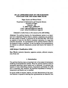
Figure 1. (a) Time-varying state realization, (b) Hankel matrices are (mirrored) submatrices of T. H0 is shaded.
since the 1950s. While most of the early work is on time-continuous linear systems and differential equations with time-varying coefficients (see e.g., [26] for a 1960 survey), time-discrete systems have gradually come into favor and are applicable to our context. Some important more recent approaches are the monograph by Feintuch/Saeks [27], in which a Hilbert resolution space setting is taken, and recent work by Kamen, Poolla and Khargonekar [28–30]. The realization theory as used in the present paper can be found in [24]. Some results are summarized below. We will be interested in systems T that admit a realization in the form of the recursion "
xk+1 = xk Ak + ukBk yk = xk Ck + uk Dk
Tk =
Ak Ck B k Dk
#
(1.2)
in which we will require the matrices fAk, Bk , Ck , Dk g to have finite (but not necessarily fixed) dimensions. Let Ak be of size dk × dk+1 , then the size of xk , i.e., the system order at point k, is equal to dk . See figure 1(a). The collection fAk, Bk , Ck , Dk g∞ −∞ is a realization of T if its entries Tij are given by 8 >
:
0, Di , Bi Ai+1 1 1 1 Aj−1 Cj ,
i>j i=j i < j.
(1.3)
Define a sequence of operators fHk g∞ −∞ with matrix representations 2
Hk =
6 6 6 6 6 4
Tk−1,k Tk−1,k+1 Tk−1,k+2 Tk−2,k Tk−2,k+1 .. . Tk−3,k .. .
111
3 7 7 7 7 7 5
.
(1.4)
We will call the Hk time-varying Hankel matrices of T, although they do not have the traditional Hankel structure unless T is a Toeplitz operator. Their matrix representations are mirrored submatrices of T (see figure 1(b)). Although we have lost the traditional anti-diagonal Hankel structure, a number of important properties are retained: 4
1. If fAk, Bk , Ck , Dk g is a realization of T, then Hk has a factorization 2 6 6
Hk = 6 6 4
Bk−1 Bk−2 Ak−1 Bk−3 Ak−2 Ak−1 .. .
3 7 7 7 [C k 7 5
AkCk+1
AkAk+1 Ck+2
] =:
111
C k Ok
.
(1.5)
and Ok can be regarded as time-varying controllability and observability operators. If the realization is minimal, then the rank of H k is equal to the system order at time k. Ck
2. Hk has shift-invariant properties. Denote by H ← k the operator Hk , with its first column deleted. Then 2
H← k
=
6 6 6 6 4
Bk−1 Bk−2 Ak−1 Bk−3 Ak−2 Ak−1 .. .
3 7 7 7A 7 k 5
[Ck+1
Ak+1 Ck+2
Ak+1 Ak+2 Ck+3
] =
111
Ck
AkOk+1 .
(1.6)
The shift-invariance property states that the row space of H← k is contained in the row space of Hk+1 . These two properties are sufficient to derive a minimal realization for T [24]. The construction consists mainly of the factorization of each Hk into minimal rank factors Ck and Ok . Once these have been determined, then the Bk and Ck are equal to the first (block)-column of Ck+1 and first row of Ok , whereas Ak can be determined by using the shift-invariance property. We will assume, throughout, that all Hk have finite rank (we will call such systems locally finite), so that the factorization is well defined. In this case, one can show that the rank of Hk is equal to the system order at point k of any minimal realization of T. Because the minimal system order of any realization is at each point k given by the rank of the Hankel matrix Hk at that point, a possible approximation scheme is to approximate each H k by one that is of lower rank (this could be done using the SVD). The approximation error could then very well be defined in terms of the individual Hankel matrix approximations as the supremum over these approximations. Because the Hankel matrices have many entries in common, it is not clear at once that such an approximation scheme is feasible: replacing one Hankel matrix by one of lower rank in a certain norm might make it impossible for the next Hankel matrix to find an optimal (in that norm) approximant such that the part that it has in common with the previous Hankel matrix will be approximated by the same matrix. This situation parallels what already occurs for linear time-invariant systems. The Hankel norm of an operator T can be defined at present as k
T kH = sup
k
Hk k .
(1.7)
k
(The definition which we will use in the paper appears in equation (2.5) below.) This definition is a generalization of the time-invariant Hankel norm and reduces to it if all H k are the same. Let Γ = diag(γi ) be an acceptable approximation tolerance, with γi > 0. If an operator Ta is such that −1 k Γ (T − Ta ) kH ≤ 1, then Ta is called a Hankel norm approximant of T, parameterized by Γ. We are interested in Hankel norm approximants of minimal system order. In this respect, we will prove the following theorem: 5
Theorem 1.1. Let T be a bounded operator which is strictly upper, strictly stable and locally finite, and let Γ be an invertible Hermitian diagonal operator. Let H k be the Hankel matrix of Γ −1T at time instant k. Suppose that the singular values of each H k decompose into two sets σ −,k and σ+,k , with lower bound of all σ −,k larger than 1, and upper bound of all σ +,k smaller than 1. Let Nk be equal to the number of singular values of H k which are larger than 1. Then there exists a strictly upper locally finite operator T a of system order at most N k at point k, such that −1 k Γ (T − Ta ) kH ≤ 1 . (The notion of strict stability is defined in section 2.1.) In fact, there is a collection of such T a . We will obtain a state space realization of a particular Ta as well (theorem 7.5). Theorem 8.8 gives a parametrization of all solutions. It is shown that no Hankel norm approximants of order lower than Nk exist. Finally, if all singular values of all H k are smaller than 1, Nehari’s theorem for time-varying systems is recovered. Such extensions have been described by Gohberg, Kaashoek and Woerdeman [31, 32].
2. PRELIMINARIES 2.1. Spaces The basic elements of our theory are generalizations of `2 -series to sequences of which the components | ,i ∈ Z Z g be an indexed collection of natural numbers ∗ have non-uniform dimensions [24]. Let fN i ∈ N which we will always take finite. The sequence N = [ Ni ]∞ −∞ = [ 1 1 1
N−1
N0
N1
N2
111
ZZ | ] ∈ N
is called an index sequence. Using N, signals u = [ 1 1 1 u−1 u0 u1 u2 non-uniform sequences which is the Carthesian product of the Ni : N
= 1 1 1 × N−1 ×
N0
111
] live in the space of
| N , × N1 × N2 × 1 1 1 ∈ C |
| Ni so that N is the dimension of N . Some of these components may have zero where Ni ∈ C i i 0 | dimension: we define C = ∅. In this way, finite dimensional vectors are also incorporated in the space of non-uniform sequences, by putting Ni = 0 for i outside a finite interval. We will write N = #(N ) to indicate the sequence of dimensions N of the sequence of spaces N .
The inner product of two non-uniform sequences f, g in N is defined in terms of the usual inner P ∗ product of (row)-vectors in Ni as ( f, g) = i ( fi , gi ) where ( fi , gi ) = fi gi is defined to be 0 if Ni = 0. y The norm of a non-uniform sequence is the standard 2-norm (vector norm) defined on this inner product: u = [ ui ]∞ −∞ :
∞
k
u k22 = (u, u) =
k
−∞
ui k22 .
The space of non-uniform sequences with index sequence N and with finite 2-norm is denoted by ` N 2 Z ). `N is a Hilbert space. | N , with N ∈ N | Z (N ∈ C 2 ∗
0 is included in N| .
y More generally, we define the product of an n × 0 matrix with a 0 × m matrix to be the zero matrix of dimensions n × m. 6
Let and N be sequences of spaces corresponding to sequences of indices M, N. We denote by N X( , N ) the space of bounded linear operators `M , N ) if and only 2 → `2 : an operator T is in X ( M N if for each u ∈ `2 , the result y = uT is in `2 , in which case the induced operator norm of T, k
T k = sup
u ≤1
k
uT k2 ,
k k2
is bounded. T ∈ X (
, N ) has a block matrix representation [Tij ]∞ i,j=−∞ such that ⇔
y = uT
yj =
ui Tij .
(2.1)
i
Consequently, we will identify T with its matrix representation and write 2
T = [Tij ]∞ i,j=−∞ =
6 6 6 6 6 6 6 6 4
..
.. .
.
. ..
T−1,−1 T−1,0 T−1,1 111 T0,−1 T00 T01 T1,−1 T10 T11 . . .. ..
111
..
3 7 7 7 7 7 7 7 7 5
(2.2)
.
(where the square identifies the 00-entry) such that it fits the usual vector-matrix multiplication rules. The block entry Tij is an Mi × Nj matrix. As explained in [24] and [23], operators T in X have an upper part and a lower part: all entries Tij above the main (0-th) diagonal and including this diagonal form the upper part, while all entries below the diagonal, including the diagonal, form the lower part. When T is a bounded operator `2M → `2N , then its upper part need not represent a bounded operator. The situation generalizes what already happens with Toeplitz operators: if the symbol of such an operator belongs to L ∞ of the unit circle, then its analytic part need not belong to L ∞ . Nonetheless, each diagonal of a bounded operator, taken by itself, is again a bounded operator with norm not exceeding the norm of the original operator. Concerning the diagonal calculus on operators between non-uniformly indexed spaces, we adopt the notation of [24] and [23]: (k)
Z
the shift operator: [ 1 1 1 x−1 Z : `2 → `2 M
Z[k]
(1)
the k-th shift rightwards in the series of spaces as in (1)
M
x0
x1
111
= [111
] Z = [ 1 1 1 x−2
111
].
] . Notice that
(k)
, N ) the space of bounded operators `2M → `2N .
U
(
, N ) the space of bounded, upper triangular operators `2M → `2N .
(
, N ) the space of bounded, lower triangular operators `2M → `N 2 .
(
111
0
M . the product of k shifts. It is an operator `M 2 → `2
(
D
x0
−1
.
X
L
x−1
−2
N , N ) the space of diagonal operators `M 2 → `2 . The norm of a member of supremum over the norms of its components.
D
will be the
Let T ∈ U , then we can formally decompose T into a sum of shifted diagonal operators as in ∞
Z[k] T[k] ,
T= k=0
7
(2.3)
where T[k] ∈ D( (k) , N ) is the k-th diagonal above the main (0-th) diagonal. Given an operator A, we can define its k-th shift in the South-East direction as A(k) = (Z[k] )∗ AZ[k] .
(2.4)
We will often encounter products (AZ)n , where A ∈ X (N , N (−1) ). These evaluate as (AZ)n
= (AZ) (AZ) 1 1 1 (AZ) = Z[n] A(n) A(n−1) 1 1 1 A(1) =: Z[n] Afng
where Afng is defined as Af0g = I , Afng = A(n)Afn−1g = A(n) A(n−1) 1 1 1 A(1) . The spectral radius r(AZ) = limn→∞ interest and is denoted by ` A .
k
(AZ)n k1/n = limn→∞
k
Afng k1/n of AZ will be of considerable
Besides the spaces X , U , L, D in which the operator norm reigns, we shall need Hilbert-Schmidt spaces X2 , U2 , L2 , D2 which consist of elements of X , U , L, D respectively, and for whom the norms of the entries are square summable. These spaces are Hilbert spaces for the usual Hilbert-Schmidt inner product. They will often be considered to be input or output spaces for our system operators. N Indeed, if T is a bounded operator `M 2 → `2 , then it may be extended as a bounded operator X2 → X2 by stacking sequences in ` 2 to form elements of X2 . This leads for example to the expression y = uT, Z , ) and y ∈ X (C Z , N ) [23]. We will use the shorthand X M for X (C Z , ), | Z | Z | Z where u ∈ X2 (C 2 2 2 is not of interest. but continue to write X 2 if the precise form of We define P as the projection operator of PL2 Z−1 as the projection operator of X2 on
on U2 , P0 as the projection operator of −1 L2 Z . X2
X2
on
D2
, and
2.2. Left D-invariant subspaces We say that a subspace
of
X2
is left D-invariant if A ∈
⇒ DA ∈
for all D ∈ D.
be Let ∆i = diag[ 1 1 1 0 0 I 0 0 1 1 1 ], where the unit operator appears at the i-th position, and let a left D-invariant subspace. Define i = ∆i , then i is also left D-invariant, and i ⊂ . If i=j, / then i ⊥ j (where orthogonality is with respect to the Hilbert-Schmidt inner product). It follows that = ⊕i i . A left D-invariant subspace is said to be locally finite if, for all i, dim i is finite. In that case, there exists a local basis for , where each basisvector is itself a basisvector of some i . The conjunction of the basisvectors of all i span . With di = dim i , we will call the sequence [ 1 1 1 d0 d1 d2 1 1 1 ] the sequence of dimensions of , and denote this as s-dim . We list some properties of D-invariant subspaces. If ⊂ X2 is left D-invariant, then so is ⊥ . If , ⊂ X2 are subspaces, then let PA ( ) indicate the projection of onto , obtained by projecting and are left D-invariant, then so are PA ( ) and PA⊥ ( ). If or is vectors of onto . If locally finite, then so is P A ( ). If two linearly independent subspaces and of X 2 are locally finite, then so is their direct sum + , so that a local basis of + can be obtained from bases of i + i , for all i. If is a left D-invariant subspace and B is a linear operator, then B is also left D-invariant. 8
2.3. Hankel operators and state spaces Let T ∈ X be a bounded operator. An abstract version of the Hankel operator maps inputs in L2 Z−1 to outputs restricted to U2 : the Hankel operator HT connected to T is the map u ∈ L 2 Z−1 7→ P(uT). Note that only the strictly upper part of T plays a role in this definition. The operators H k of equation (1.4) are ‘snapshots’ of it: Hk can be obtained from HT by considering a further restriction to inputs ∆k u of which only the k-th row is non-zero: the operator (∆k ⋅ )HT is isomorphic to H k. [The isomorphism consists of removing zero rows of ∆k u and y = (∆k u)HT , and writing the resulting `2 -sequences as one-sided sequences.] The canonical realization theory in [24] is based on distinguishing characteristic spaces in L2 Z−1 and U2 , which are the range and kernel of HT and (HT )∗ : (T) = ran (H∗T ) = fPL2 Z−1 (yT∗ ) : y ∈ U2 g ⊂ L2 Z−1,
– the natural input state space
0 (T)
– the natural output state space
= ran (HT ) = fP(uT) : u ∈ L2 Z−1g ⊂ U2 .
and 0 are not necessarily closed; These spaces are left D-invariant: D ⊂ , D 0 ⊂ 0 . and 0 are left D-invariant subspaces, which have shift-invariance properties as are their closures explained in the cited paper. Throughout the paper, it will be assumed that T is such that (T) and 0 (T) are locally finite subspaces. Such T will be called locally finite transfer operators. 2.4. Hankel norm Let the Hankel norm of T be defined as the operator norm of its Hankel operator: k
T kH = k HT k .
(2.5)
This definition is equivalent to the definition in (1.7). It is a norm on ZU , but a seminorm on X . We will also employ another norm, the diagonal 2-norm. Let T i be the i-th row of a block matrix representation T ∈ X , then D∈D: T∈X :
D kD2 = supi k Di k, 2 ∗ k T kD 2 = k P0 (TT ) kD 2 = supi k
k
Ti T∗i k .
For diagonals, it is equal to the operator norm, but for more general operators, it is the supremum over the ‘vector’ 2-norms of each row of T. Proposition 2.1.
The Hankel norm satisfies the following inequalities: T∈X :
k
T kH ≤
T ∈ ZU :
k
T kD2 ≤
k
Tk
k
(2.6)
T kH .
(2.7)
Proof The first norm inequality is proven by k
T kH = supu∈L2 Z−1 ,k u kHS ≤1 ≤ supu∈L2 Z−1 ,k u kHS ≤1 ≤ supu∈X2 ,k u kHS ≤1
For the second norm inequality, we first prove k
k
P(uT) kHS k uT kHS = k uT kHS k
k
Tk.
T k2D2 ≤ supD∈D2 , k D kHS ≤1
T k2D2 = k P0 (TT∗ ) k2D2 = supD∈D2 , k D kD2 ≤1 = supD∈D2 , k D kHS ≤1 ≤ supD∈D2 , k D kHS ≤1 9
k
DP0 (TT∗ )D∗ kD2 ∗ ∗ k DP0 (TT )D kHS ∗ ∗ k DTT D kHS . k
DTT∗ D∗ kHS . Indeed,
Then (2.7) follows, with use of the fact that T ∈ ZU , since the latter term is majorized by k
T k2D2 ≤ supD∈D2 , k D kHS ≤1 = supD∈D2 , k D kHS ≤1 = supD∈D2 , k D kHS ≤1 ≤ supu∈L2 Z−1 , k u kHS ≤1
DTT∗ D∗ kHS ∗ ∗ ∗ k DZ TT ZD kHS 2 3∗ ∗ ∗ k P(DZ T) P(DZ T) kHS ∗ = k P(uT) [P(uT)] kHS
k
T k2H:
k
k
T k2H .
We see that the Hankel norm is not as strong as the operator norm, but is stronger than the row-wise uniform least square norm. 2.5. Realizations If the natural input state space and the natural output state space have a locally finite basis then realizations of type (1.2) can be derived. Turning to this type of realizations, we can assemble the matrices fAk g, fBkg etc. as operators on spaces of sequences of appropriate dimensions, by defining A = diag(Ak), B = diag(Bk ), C = diag(Ck ) and D = diag(Dk ). Let `2M be the space of input sequences, `2N the space of output sequences, and let us define = f k : k ∈ ZZ g as the sequences of spaces to which the state x = [ 1 1 1 x0 x1 x2 1 1 1 ] belongs. If all operators fAk g, fBkg, etc. are uniformly bounded over k, then A, B, etc. may be viewed as bounded diagonal operators A ∈ B ∈
( , D( , D
C ∈ D ∈
(−1) ) , (−1) ) ,
( ,N), D( ,N), D
(2.8)
which together define the dynamical equations "
xZ−1 = xA + uB y = xC + uD
T=
A C B D
#
(2.9)
With `A the spectral radius of the operator AZ, we shall say that the realization (2.9) is strictly stable if `A < 1. In that case, the operator (I − AZ)−1 exists as a bounded operator and elimination of x in (2.9) leads to x = uBZ(I − AZ)−1 (2.10) so that T can be written in terms of fA, B, C, Dg as T = D + BZ(I − AZ)−1 C . The realization (2.9) can be generalized further, by considering inputs and outputs in respectively, for which again the same relations hold: "
xZ−1 = xA + uB y = xC + uD
T=
A C B D
M
X2
and
N
X2
,
#
(2.11)
If `A < 1, then also x = uBZ(I − AZ)−1 ∈ X2B . By projecting both equations in (2.11) onto the k-th diagonal, and using the fact that A, B, C, D are diagonal operators, a generalization of the recursive realization (1.2) is obtained as x(−1) [k+1] = x[k] A + u[k] B (2.12) y[k] = x[k] C + u[k]D (see figure 2(b).) Note the diagonal shift in x(−1) [k+1] . Two more representations for T can be derived from (2.12). For u ∈ X2 , we define the past and future signals, with respect to the 0-th diagonal of u, by the projection of u onto L 2 Z−1 and U2 respectively, so that u = up + uf ∈ L2 Z−1 ⊕ U2 , with 10
x(2) [−2] u(2) [−2]
T(2) x(1) [−1]
u(1) [−1] u
T
T(1)
Tp
y(2) [−2] KT
up
T
u[0]
y(1) [−1]
T(−1)
y[0]
G uf
yf
ET
y(−1) [1]
uf
yf
ET Tf
x(−2) [2] (a)
yp
x[0]
HT
x(−1) [1] u(−1) [1]
KT
up
P(⋅F∗ )
x[0]
y
yp
(b)
(c)
(d)
Figure 2. (a) Causal transfer operator T, (b) realization T, (c) splitting into past and future signals, (d) representation by T p and Tf .
up = PL2 Z−1 (u) = Z−1 u[−1] + Z−2 u[−2] + 1 1 1 and uf = P(u) = u[0] + Zu[1] + Z2 u[2] + 1 1 1. If the same is done to y ∈ X2 , then y = uT is equivalent to y = yp + yf , with yp = up KT yf = up HT + uf ET
KT = PL2 Z−1 ( ⋅ T) ET = P( ⋅ T) 2
where
L2
Z−1
(2.13)
and where HT is the Hankel operator defined before (see figure 2(c)). If uf = 0, then yf = up HT . The following construction shows that the existence of a realization implies that H T can be factored into two operators. According to (2.12), and assuming `A < 1, x[0] is equal to x[0] = P0 (x) = P0 ( u BZ(I − AZ)−1 ) = P0 ( up BZ(I − AZ)−1 ) + P0 ( uf BZ(I − AZ)−1 ) = P0 ( up BZ(I − AZ)−1 ) .
(2.14)
fk g If uf = 0 then, for k ≥ 0, y[k] = x[k] C = x(k) C, so that [0] A
P
∞ [k] yf = 0 Z y[k] P∞ [k] (k) fkg = C 0 Z x[0] A P∞ k = 0 x[0] (AZ) C = x[0] (I − AZ)−1 C .
(2.15)
Hence HT has the factorization HT = P0 ( ⋅ F∗ ) G, with F∗ = BZ(I − AZ)−1 and G = (I − AZ)−1 C. Representation (2.13) is thus equivalent to the equations 2
3
x[0] yp = up Tp yf = [ x[0] uf ]Tf
with
8 >
:
Tf
2
P ( ⋅ F∗ ) " 0 # G = ET
KT
3
(2.16)
See figure 2(d). We call the decomposition of T into the operators Tp and Tf a state splitting of T. 2.6. Controllability and observability operators An important aspect of the factorization HT = P0 ( ⋅ F∗ ) G is its minimality, since this will imply the minimality of the sequence of dimensions of x and thus the minimality of the realization. A realization 11
is said to be controllable if the range of P 0 ( ⋅ F∗ ) L2 Z−1 is dense in D2B , and uniformly controllable if its range is all of D2B , that is, if P0 (L2 Z−1 F∗ ) = D2 . If P0 ( ⋅ F∗ ) is regarded as an operator from −1 → D , then its adjoint is ⋅ F with domain D , and the realization is controllable if DF = 0 ⇒ L2 Z 2 2 D = 0 (D ∈ D2 ), that is, if the gramian P0 (FF∗ ) > 0. The realization is uniformly controllable if P0 (FF∗ ) is uniformly positive, by which we mean ∃ ε > 0 : P 0 (FF∗ ) ≥ ε I. Observability is defined in much the same way. A realization is observable if P0 (U2 G∗ ) is dense in D2B , which is equivalent to P0 (GG∗ ) > 0, and uniformly observable if P0 (U2 G∗ ) = D2B , i.e., P0 (GG∗ ) is uniformly positive. A realization which is both controllable and observable is said to be minimal. If a realization has ` A < 1 and is uniformly observable, then the input state space is (T) = D 2B F = D2B (I−Z∗ A∗ )−1 Z∗ B∗ . Similarly, for a uniformly controllable realization the output state space is 0 (T) = D2B G = D2B (I − AZ)−1 C. This shows that if the realization is minimal, then s-dim = s-dim 0 is equal to the sequence of dimensions of , the space of state sequences. It is possible to prove the converse, i.e., to show that if s-dim (T) = s-dim 0 (T) = [ 1 1 1 d0 d1 d2 1 1 1 ] is a uniformly bounded sequence of dimensions, then there exist realizations of T with dk = dim k equal to the system order at point k [24]. This number is equal to the rank of Hk . We will call the sequence the minimal system order of T. If T admits a locally finite realization, then it is always possible to choose this realization to be either uniformly controllable or uniformly observable, although it may not be possible to have both (this is typically the case if the range of HT is not closed). The action of the operators P0 ( ⋅ F∗ ) and G can be made more ‘visual’ by considering a representation as sequences of diagonals [24]. From (2.14) and (2.15) we obtain x[0] = P0 up BZ(I − AZ)−1 = P0 [Z−1 u[−1] + Z−2 u[−2] + 1 1 1] [BZ + BZ AZ + BZ AZ AZ + 1 1 1] (2) −2 (1) + Z2 B(2) A(1) + Z3 B(3) A(2) A(1) + 1 1 1] −1 = P0 [u(1) [−1] Z + u[−2] Z + 1 1 1] [ZB 2
=
u(1) [−1]
u(2) [−2]
u(3) [−3] 1 1 1
[ y[0]
y(−1) [1]
y(−2) [2]
3
B(1) 6 (2) (1) 7 6B A 7 6 7 6 B(3) A(2) A(1) 7 4 5 .. .
and
The operators
2 (1) B C
:=
111
] = x[0] C AC(−1) AA(−1)C(−2)
111
.
3
6 (2) (1) 7 6B A 7 6 7 6 B(3) A(2) A(1) 7 4 5
O
:= C AC(−1) AA(−1) C(−2)
111
.. .
are representations of P0 ( ⋅F∗ ) and G in ‘diagonal sequence’ spaces `2 (D) which are isomorphic to −1 and U . C and O as defined in the introduction (equation (1.5)) are obtained from C and O by L2 Z 2 k k taking the k-th entry along each diagonal of C and O. The controllability gramian P 0 (FF∗ ) is equal to C ∗ C . Likewise, the observability gramian is P 0 (GG∗ ) = OO∗ . 2.7. Lyapunov Equations Another notion that we shall need is that of state transformations. If fA, B, C, Dg is a strictly stable realization of a system with transfer operator T, then an equivalent strictly stable realization is found 12
by applying a state transformation xˆ = xR on the state sequence x of the system with a bounded and boundedly invertible diagonal operator R. The transition operator T is then transformed to "
T0 =
#"
R I
A C B D
#"
#
(R(−1) )−1 I
.
(Note the diagonal shift in (R (−1) )−1 ). It is easy to see that `RA(R(−1) )−1 = `A , hence that strict stability is preserved under the transformation. State transformations are often used to bring a transition operator into some desirable form. This then leads to equations of the famous Lyapunov or Lyapunov-Stein type. For example, the Lyapunov equation M(−1) = A∗ MA + B∗ B ,
M ∈ D( , )
(2.17)
arises in the transformation of a strictly stable and uniformly controllable realization to input normal form: one for which A∗ A + B∗ B = I. If the original realization is uniformly controllable, then a boundedly invertible state transformator R can be found such that A 1 = RA(R(−1) )−1 , B1 = B(R(−1) )−1 and A∗1 A1 + B∗1 B1 = I . Substitution leads to equation (2.17), with M = R ∗ R, and hence it suffices to solve this equation for M and to verify that M is boundedly invertible, in which case a factor R is boundedly invertible too. Equation (2.17) will have the unique solution ∞
M =
(1)
(Afkg)∗ B∗ B
(k)
A fk g
k=0
provided `A < 1, in which case the sum converges in operator norm. By taking the k-th entry of each diagonal which appears in (2.17), this equation leads to M k+1 = A∗k Mk Ak + B∗k Bk , which can be solved recursively if an initial value for some Mk is known. Finally, if C is the controllability operator of the given realization, then M = C ∗ C is the solution of (2.17), which shows that M is boundedly invertible if the realization is uniformly controllable. Likewise, if the realization is strictly stable and uniformly observable (O is such that Q = OO ∗ is boundedly invertible), then Q is the unique bounded solution of the Lyapunov equation Q = AQ(−1) A∗ + CC∗ (2.18) and with the factoring of Q = RR∗ this yields a boundedly invertible state transformation R such that A1 = R−1AR(−1) , B1 = BR(−1) , C1 = R−1C, and A1 A∗1 + C1 C∗1 = I . The resulting fA1 , B1 , C1 , Dg then form an output normal realization for the operator. In section 6 we shall assume that the operator to be approximated is indeed specified by a realization in output normal form. If T is locally finite, then it is always possible to obtain a realization in output normal form by constructing it from an orthonormal basis of the output state space 0 (T) [24]. For a general upper operator T, one other way to obtain such a realization is by breaking off the diagonal series representation of T at a sufficiently P high order, T ≈ N0 Z[k] T[k] , in which case we can take as a trivial (possibly non-minimal) realization 2
"
Ak Ck B k Dk
#
=
6 6 6 6 6 6 6 6 6 6 4
0
0
1 0
1 .. .
.. 0
0 Tk,k+N
111
. 1 0 Tk,k+1
0 .. . .. . 0 1 Tk,k
3 7 7 7 7 7 7 7 7 7 7 5
In this case, `A = 0 (A is nilpotent) and the realization is strictly stable, while it is also in output normal form: AA∗ + CC∗ = I. This realization is a high-order approximating model of T, which can subsequently be reduced to a low-order Hankel-norm approximant by application of theorem 1.1. 13
3. J-UNITARY OPERATORS In the sequel, we shall be dependent on the properties of certain unitary and J-unitary operators. These are well-known for their time-invariant analogs, and some of the generalizations have already been derived for the context of upper operators which act on ‘constant size’ sequences of spaces in [16,23]. The present section considers the more general case of non-uniform sequences of spaces. 3.1. J-unitary operators and J-unitary realizations If an operator is at the same time unitary and upper, we shall call it an inner operator. In this paper we shall make extensive use of operators Θ that consist of 2 × 2 block entries which are upper operators such that Θ is J-unitary in a generalized sense. To introduce this notion properly, we must define a splitting of the sequence of input spaces of Θ into two sequences 1 and N1 , a splitting of the sequence of output space sequences into two sequences 2 and N2 , and define corresponding signature sequences J1 and J2 : "
Θ=
Θ11 Θ12 Θ21 Θ22
#
"
,
#
IM1
J1 =
"
,
−IN1
J2 =
IM2
#
−IN2
.
(3.1)
M2 1 2 Θ decomposes in four blocks, mapping ` 2M1 ⊕ `N ⊕ `N 2 to `2 2 . If each of these maps is upper, we say that Θ is block-upper. Θ will be called J-unitary relative to this splitting in blocks, when
Θ∗ J1 Θ = J2
ΘJ2 Θ∗ = J1 .
and
We will not say that such a Θ is J-inner unless additional constraints which go beyond the scope of the present paper are satisfied (see also [23]). We will now show that a state realization Θ which is J-unitary in a certain sense leads to a J-unitary transfer operator Θ. Let be the sequence of spaces of the state of Θ , and let = + ⊕ − be a decomposition of into two sequences of spaces. Let "
#
IB+
JB =
(3.2)
−IB−
be a corresponding signature matrix, which we call in this context the state signature sequence of Θ . We have the following connection between a realization matrix Θ and the transfer operator Θ. Theorem 3.1.
Let J1 , J2 and JB"be signature sequences with dimensions as given in (3.1), (3.2). # α γ β δ
If a state realization operator Θ =
"
Θ∗ "
Θ
is strictly stable and satisfies #
JB J1
"
Θ=
" ∗
J2
(3.3)
J2
#
J(−1) B
#
J(−1) B
Θ =
#
JB J1
(3.4)
then the corresponding transfer operator Θ = δ + βZ(I − αZ) −1 γ will be J-unitary in the sense that Θ∗ J1 Θ = J2 ,
ΘJ2 Θ∗ = J1 .
(3.5)
With ‘#’ indicating the sequence of dimensions of a space sequence, we will have in addition that # + +# 1 = # # − + #N 1 = # 14
(−1) + (−1) −
+# 2 + #N 2 .
(3.6)
Proof The theorem is readily verified by evaluating J2 − Θ∗J1 Θ and J1 − ΘJ2 Θ∗, e.g., J2 − Θ∗ J1 Θ = J2 − δ∗ J1 δ + γ ∗ (I − Z∗ α∗ )−1 Z∗ α∗ JB γ + γ ∗ JB αZ(I − αZ)−1 γ + − α∗ JB αgZ(I − αZ)−1 γ − γ ∗ (I − Z∗ α∗ )−1 Z∗ fJ(−1) B = γ ∗ JB γ + γ ∗ (I − Z∗ α∗ )−1 fZ∗ α∗ JB + JB αZ − JB − Z∗ α∗ JB αZg(I − αZ)−1 γ since β∗ J1 δ = −α∗ JB γ , β∗ J1 β = J(−1) − α∗ JB α and J2 − δ∗ J1 δ = γ ∗ JB γ , and hence B J2 − Θ∗ J1 Θ = γ ∗ (I − Z∗ α∗ )−1 f(I − Z∗ α∗ )JB (I − αZ) + + Z∗ α∗ JB + JB αZ − JB − Z∗ α∗ JB αZg(I − αZ)−1 γ = 0. The second equality of (3.5) follows by an analogous procedure. Equations (3.3) and (3.4) show that Θ is invertible, so that for each time instant k, the total positive signature at the left hand side of each equation is equal to the total positive signature at the right hand side (the so-called inertia theorem). A similar observation holds for the total negative signature at each point k. This is expressed in (3.6). 3.2. Interpolation properties of J-unitary operators A J-unitary upper operator has the special property that it maps its input state space to [ U 2 Proposition 3.2. Θ, then
U2
].
If fα, β, γ , δg is a J-unitary state realization for a J-unitary block-upper operator (I − Z∗ α∗ )−1 Z∗ β∗ J1 Θ ∈ [U
U
]
(3.7)
that is, (I − Z∗ α∗ )−1 Z∗ β∗ J1 , which consists of two strictly lower blocks, is mapped by Θ to block upper. Note that the input state space of Θ is of (3.7) and using (3.3) reveals that
(Θ) = D 2 (I−Z∗ α∗ )−1 Z∗ β∗ ∈ [L2 Z−1
L2
Z−1 ]. Proof Evaluation
(I − Z∗ α∗ )−1 Z∗ β∗ J1 δ + βZ(I − αZ)−1 γ = (I − Z∗ α∗ )−1 Z∗ −α∗ JB + (J(−1) − α∗ JB α)Z(I − αZ)−1 γ B (−1) = (Z − α∗ )−1 −α∗ JB (I − αZ) + JB Z − α∗ JB Z (I − αZ)−1 γ
= JB (I − αZ)−1 γ
∈ [U
U
(3.8)
].
This property has an ‘interpolation’ interpretation which is explained in detail (for the less general context of uniform sequences of spaces) in [23]. The interpolation principle will provide us with the necessary factorizations and will be used in section 6. 3.3. Scattering operators Two of the relations in the expressions Θ ∗ J1 Θ = J2 , ΘJ2 Θ∗ = J1 are Θ∗22 Θ22 = I + Θ∗12 Θ12 and Θ22 Θ∗22 = I + Θ21 Θ∗21 . Hence Θ22 is a one-to-one map of `2N1 onto `2N2 , which ensures that it is boundedly invertible [16, lemma 5.2]. Associated to Θ is an operator Σ, "
Σ=
Σ11 Σ12 Σ21 Σ22 15
#
Θ11
a1
a2
Σ11
a1
Θ12
Σ12
Θ21 b1
b1
b2
Θ22 Θ
a2
Σ21
Σ22
b2
Σ
Figure 3. Relation between a J-unitary operator Θ and its corresponding unitary operator Σ.
such that [a1 b2 ]Σ = [a2 b1 ] ⇔ [a1 b1 ]Θ = [a2 b2 ] , (see figure 3). Σ can be evaluated in terms of the block-entries of Θ as "
Σ=
I −Θ12 0 I
#"
Θ11 0 0 Θ−1 22
#"
I 0 Θ21 I
#
"
=
−1 Θ11 − Θ12 Θ−1 22 Θ21 −Θ12 Θ22 −1 −1 Θ22 Θ21 Θ22
#
(3.9)
It is well-known and straightforward to prove that from the J-unitarity of Θ it follows that Σ is unitary. Σ is known as a scattering operator, while Θ is called a chain scattering operator. Σ and Θ constitute the same linear relations between the quantities a 1 , a2 , b1 , b2 . However, Σ has the connotation of visualizing the ‘positive energy flow’ between these quantities: a 1 a∗1 + b2 b∗2 = a2 a∗2 + b1 b∗1 , whereas for Θ, a1 a∗1 − b1 b∗1 = a2 a∗2 − b2 b∗2 . In engineering literature, a1 and b2 are known as incident waves, whereas a2 and b1 are reflected waves. One fact which will be essential for the approximation theory in the later chapters is that, although Θ has block-entries which are upper, Θ−1 22 need not be upper but can be of mixed causality, so that the block-entries of Σ are in general not upper. 3.4. Realization for Σ The realization Θ for Θ satisfies (3.3) and (3.4). The state space sequence decomposes into two complementary space sequences = + ⊕ − of locally finite dimensions. Let any state sequence x ∈ X2B and Θ be partitioned accordingly into x = [x+ x− ] with x+ ∈ X2B+ and x− ∈ X2B− and [x+
x−
a1
b1 ] Θ = [x+ Z−1
x− Z−1
a2
b2 ] .
(3.10)
Θ has a corresponding partitioning into
Θ =
x+ x−
2
6 6 6 6 a1 4
b1
x+ Z−1
x− Z−1
a2
b2
α11 α21
α12 α22
γ11 γ21
γ12 γ22 7 7
β11 β21
β12 β22
δ11 δ21
3
7. 7 δ12 5
(3.11)
δ22
A reordering of rows and columns with respect to their signatures converts Θ into a genuine squareblock J-unitary operator, i.e., each matrix 2 6 6 6 6 4
α11 β11
γ11 δ11
α12 β12
γ12 δ12
α21 β21
γ21 δ21
α22 β22
δ22
16
3
7 7 7 γ22 7 5 k
+ )k
(
+ +
1 )k
( (
(
−
Θk
− +
1 )k
(
− )k
−
+ )k+1
(
(
+
(
−
(
2 )k 2 )k
+ +
1 )k
( (
(
− )k+1
(
− )k
−
Σk
− +
1 )k
(a)
+ )k
−
+ )k+1
(
+
(
−
(
2 )k 2 )k
− )k+1
(b)
Figure 4. (a) The spaces connected with a realization for a J-unitary block-upper operator Θ which transfers 1 × 2 1 to 2 2 × 2 2 . The state transition operator is marked as Θ. Θ transfers, at stage k, 2 ( + )k × ( − )k × ( 1 )k × ( 1 )k to ( + )k+1 × ( − )k+1 × ( 2 )k × ( 2 )k . (b) The corresponding scattering situation.
is a square and J-unitary matrix with signature [I(B+ )k ⊕(M1 )k +˙ submatrix " # α22 β22
γ22 δ22
− I(B− )k ⊕(N1 )k ]. In particular, each
k
of Θ k is square and invertible, and because Θ is J-unitary, the block-diagonal operator constructed from these submatrices is boundedly invertible as well. It follows that the following block-diagonal operators are well-defined (cf. equation (3.9)): "
"
"
"
F11 H11 G11 K11 F12 H12 G12 K12 F21 H21 G21 K21 F22 H22 G22 K22
#
#
"
# "
α γ α = 11 11 − 12 β11 δ11 β12 "
=− #
"
= #
"
=
α12 β12
γ12 δ12
α22 β22
γ22 δ22
α22 β22
γ22 δ22
#"
#−1 " #−1
γ12 δ12
#"
α22 β22
γ22 δ22
α21 β21
γ21 δ21
α22 β22
#−1
γ22 δ22
#−1"
#
α21 β21
γ21 δ21
#
(3.12)
and we obtain the relation [x+
x− Z−1
a1
where
Σ=
x+ x− Z−1 a1 b2
2 6 6 6 6 4
b2 ] Σ = [x+ Z−1
x−
a2
b1 ]
x+ Z−1
x−
a2
F11 F21
F12 F22
H11 H21
H12 H22 7 7
G11 G21
G12 G22
K11 K21
K22
b1
(3.13)
3
7. 7 K12 5
(3.14)
See figure 4. Σ is a kind of generalized or implicit realization for Σ, which can be obtained after elimination of x − and x+ . It can be interpreted as a realization having an ‘upward’ state sequence x− and a downward state sequence x+ , as depicted in figure 5. Be that as it may, the important point is the existence of Σ and its unitarity: ΣΣ∗ = I ; Σ∗Σ = I 17
a1,−2 b1,−2
a1,−1 b1,−1
a2,−1 b2,−1
Σ −1 x+,0
a1,0 b1,0
a1p
a2p
b1p
b2p x+[0]
x−,0 Σ0
a1,1 b1,1
Σp
a2,−2 b2,−2
Σ −2
Σ1
a2,0 b2,0
x−[0]
a1f
a2f
b1f
b2f
a2,1 b2,1
Σf
(a)
(b)
Figure 5. (a) The state transition scheme for Σ , with 2 -sequences as inputs. (b) The decomposition of Σ into a past operator Σ p and a future operator Σ f linked by the state [x +[0] x−[0] ]. This summarizes the figure on the left for all time.
which is easily derived from the J-unitarity of Θ . 3.5. Existence of Σp and Σf In section 2, we defined for a signal u ∈ X2 the decomposition u = u p +uf , where up = PL2 Z−1 (u) ∈ L2 Z−1 is the ‘past’ part of the signal (with reference to its 0-th diagonal), and uf = P(u) ∈ U2 is its ‘future’ part. We also showed how a causal operator T with state realization T can be split into a past operator Tp which maps up to [x[0] yp ] and a future operator Tf which maps [x[0] uf ] to yf . In the present context, let the signals a 1 , b1 , a2 , b2 and the state sequences x+ , x− be in X2 and be related by Θ as in (3.10). With the partitioning of a 1 , etc., into a past and a future part, Θ can be split into operators (⋅)Θp and (⋅)Θf via
[x+[0]
[a1p b1p ] Θp = [x+[0] x−[0] x−[0] a1f b1f ] Θf = [a2f b2f ] .
a2p
b2p ]
(3.15)
We wish to define operators (⋅)Σp , (⋅)Σf : [x−[0] a1p b2p ] Σp = [x+[0] [x+[0] a1f b2f] Σf = [x−[0]
a2p b1p ] a2f b1f ]
which are the (non-causal) scattering operators corresponding to Θp and Θf , respectively. (See figure 5(b).) The existence of Σp and Σf is asserted in the following proposition. Proposition 3.3. Let Θ ∈ U be a locally finite J-unitary operator with strictly stable J-unitary realization Θ . Then the associated scattering operators Σ p and Σf are well defined and unitary.
Proof The proof follows an argument that parallels the proof of existence of Σ from Θ, but now
applied to restrictions of Θp and Θf to inputs and outputs for which only the k-th row is non-zero, 18
for all k in turn (cf. the connection of Hk with HT ). In this proof, the operator Θ is considered as an M2 1 2 ⊕ `N operator from `2M1 ⊕ `N 1p,k be the restriction of 2 to `2 2 . Fix some time point k, and let 1 to the interval (−∞, k − 1), and likewise for N1p,k . Let the operator Θpk define the state splitting M N M N at time point k, mapping signals belonging to ` 2 1p,k ⊕ `2 1p,k to +,k ⊕ −,k ⊕ `2 2p,k ⊕ `2 2p,k : Θpk :
[a1p,k b1p,k ] 7→ [x+,k x−,k a2p,k b2p,k ] .
It has a state realization, fαi , βi , γi , δi g∞ −∞ say, which coincides with the state realization of Θ up to the index k − 2. For the index k − 1, the computed x+,k and x−,k have to be considered as outputs (not as states), and hence the realization at that point has vanishing α k−1 , βk−1 , leaving a square J-unitary pair "
γk−1 δk−1
#
= Θ k−1 .
From point k on, all state matrices of Θpk have vanishing dimensions. Because Θ pk now has a J-unitary realization, it is a J-unitary operator itself (by theorem 3.1), and the corresponding scattering map Σpk exists as well as a bounded, unitary operator linking Σpk :
[x−,k a1p,k b2p,k ] 7→ [x+,k a2p,k b1p,k ]
Finally, returning from `2 to the X2 context, Σp is obtained by piecing the Σ pk together into one global operator. A parallel, dual reasoning holds for Σf .
4. SUMMARY OF THE APPROXIMATION PROCEDURE In the present section we shall outline the overall procedure to obtain a reduced-order approximant, and put the various facts needed in perspective. Details are proven in subsequent sections. Let and N be sequences of spaces, and let T ∈ U ( , N ) be a given bounded, locally finite, strictly upper operator which has a strictly stable realization fA, B, C, 0g. We assume, without loss of generality, that this realization is uniformly observable. Let Γ be a diagonal and hermitian operator belonging to D( , ). We shall use Γ as a measure for the local accuracy of the reduced order model. It will also parametrize the solutions. We will look for a bounded operator T 0 such that k
Γ−1(T − T 0 ) k ≤ 1 ,
(4.1)
and such that the strictly upper part of T 0 has state space dimensions of low order — as low as possible for a given Γ. Let Ta be the strictly causal part of T 0 . Proposition 2.1 shows that k
Γ−1(T − Ta ) kH = ≤
Γ−1(T − T 0) kH −1 0 k Γ (T − T ) k ≤ 1 , k
(4.2)
so that Ta is a Hankel-norm approximant when T 0 is an operator-norm approximant. A generalization of Nehari’s theorem to the present setting would state that inf k Γ−1(T−T 0 ) k over all possible extensions T 0 of Ta actually equals k Γ−1(T − Ta ) kH (see section 9). The construction of an operator T 0 satisfying (4.1) consists of three steps. We start by determining a (minimal) factorization of T in the form T = ∆∗ U (4.3) 19
where ∆ and U are upper operators which have finite state space dimensions of the same size as that of T, and U is inner. We call this factorization an external factorization of T, and show in section 5 that it always exists if the realization fA, B, C, 0g for T is strictly stable and is chosen to be in output normal form, i.e., such that AA∗ + CC∗ = I, a condition that is always possible to achieve by a state transformation starting from an initial realization which is uniformly observable (see the Lyapunov equation (2.18)). It will follow from the construction that a state space realization for U shares A and C with T. Next, we look (in section 6) for a locally finite J-unitary operator Θ with 2 × 2 block-upper entries chosen such that [U∗ − T∗ Γ−1] Θ = [A 0 − B 0] (4.4) consists of two upper operators. We will show that a solution to this problem exists if certain conditions on a Lyapunov equation associated to Γ −1T are satisfied (this can always be the case for judiciously chosen Γ). Θ will again be locally finite. There is an underlying generalized interpolation problem leading to Θ, which will also be elucidated in section 6. The procedure is an extension of the method used in [23] to solve the time-varying Nevanlinna-Pick problem. With a block-decomposition of Θ as in (3.1), it is known that Θ 22 is boundedly invertible so that ∗ ∗ −1 0 Σ12 = −Θ12 Θ−1 22 exists and is contractive. From (4.4) we have B = −U Θ12 + T Γ Θ22 . As the third step in the construction of the approximant T a , define ∗
Substitution leads to
T 0 = B 0 Θ−1 22 Γ .
(4.5)
T 0 ∗ Γ−1 = T∗ Γ−1 − U∗ Θ12 Θ−1 22 = T∗ Γ−1 − U∗ Σ12
(4.6)
and it follows that (T ∗ − T 0 ∗ )Γ−1 = −U∗ Σ12 . Because Σ12 is contractive and U unitary, we infer that k
(T∗ − T 0∗ )Γ−1 k = =
− U∗ Σ12 k k Σ12 k ≤ 1 , k
(4.7)
∗
is indeed an approximant with an admissible modeling error. In view of the so that T 0 = B 0 Θ−1 22 Γ target theorem 1.1, it remains to show that the strictly causal part of T 0 has the stated number of states and to verify the relation with the Hankel singular values of Γ −1T. This will done in section 6 and 7. The definition of T 0 in (4.5) can be generalized by the introduction of a contractive operator SL which parameterizes the possible approximants. This is the subject of section 8. We first show that T has indeed a factorization T = ∆∗ U, and derive expressions for Θ satisfying the interpolation condition (4.4).
5. EXTERNAL FACTORIZATION FOR T
Theorem 5.1. Let T be an upper operator which has a strictly stable locally finite and uniformly observable state space realization fA, B, C, Dg. Then there exists a factorization of T as T = ∆∗ U , 20
(5.1)
where ∆ and U are upper operators, again locally finite and strictly stable, and U is inner, i.e., upper and unitary.
Proof We start from a realization of T in output normal form, such that AA∗ + CC∗ = I ,
(5.2)
i.e., at each time point k the equation AkA∗k + Ck C∗k = I is satisfied. We will assume that A is a diagonal (−1) B and T is an operator from `2M to `2N . For each time instant k, augment operator mapping `B 2 to `2 the state transition matrices [Ak Ck ] of T with as many extra rows as needed to yield a unitary (hence square) matrix Uk: "
Uk
=
k
(
U )k
k+1
Ak (BU )k
Nk
#
Ck . (DU )k
(5.3)
The added rows introduce a space ( U )k with the property # k + #( U )k = # k+1 + #Nk . From AkA∗k +Ck C∗k = I it follows that # k+1 +#Nk ≥ # k, hence #( U )k ≥ 0. Assemble the individual matrices fAk , (BU )k , Ck , (DU )k g in diagonal operators fA, BU , C, DU g, and define U by taking the corresponding operator U as a state space realization for U; U = DU + BU Z(I − AZ)−1 C. U is well-defined and upper because `A < 1, and it is unitary because it has a unitary realization (this fact is a specialization of theorem 3.1). It remains to show that ∆ = UT ∗ is upper. This follows by direct computation of ∆, in which we make use of the relations AA∗ + CC∗ = I, BU A∗ + DU C∗ = 0: 32
2
∆ = UT∗ = DU + BU Z(I − AZ)−1 C D∗ + C∗ (I − Z∗ A∗ )−1 Z∗ B∗ 2 3 = DU + BU Z(I − AZ)−1 C D∗ + DU C∗ (I − Z∗ A∗ )−1 Z∗ B∗ + + BU Z(I − AZ)−1 CC∗ (I − Z∗ A∗ )−1 Z∗ B∗ 2 3 = DU + BU Z(I − AZ)−1 C D∗ − BU A∗ (I − Z∗ A∗ )−1 Z∗ B∗ + + BU Z(I − AZ)−1 (I − AA∗ ) (I − Z∗ A∗ )−1 Z∗ B∗ .
3
Now, we make use of the relation Z(I − AZ)−1 (I − AA∗ )(I − Z∗ A∗ )−1 Z∗ = (I − ZA)−1 + A∗ (I − Z∗ A∗ )−1 Z∗ which is easily verified by pre- and postmultiplying with (I−ZA) and Z(I−Z ∗ A∗ ), respectively. Plugging this relation into the expression for ∆, it is seen that the anti-causal parts of the expression cancel, and we obtain 2 3 ∆ = DU + BU Z(I − AZ)−1 C D∗ + BU (I − ZA)−1 B∗ = DU D∗ + BU B∗ + BU (I − ZA)−1 Z(AB∗ + CD∗ ) .
Underlying theorem 5.1 is the interpolation property 3.2, specialized to inner operators. For a minimal realization of T, the space D2B (I − AZ)−1 C may be seen as the natural output state space 0 = 0 (T) of T. The procedure in the theorem amounts to finding a unitary U with an output state space that at least contains the output state space of T. The interpolation property then ensures (U) U ⊃ 0 , i.e., 0U
∗
⊂ 21
(U)
(a)
0
0
0
1
1
1
2
2
2
3
3
3
(b)
T
(c)
U
∆
Figure 6. (a) The state space structure of an example T, (b) The structure of the corresponding inner factor U and (c) of ∆.
and it follows that ∆ ∗ = TU∗ must be lower triangular: P(L2 Z−1∆∗ ) = 0. The latter is checked as follows: P(L2 Z−1 ∆∗ ) = P(L2 Z−1 TU∗ ) = P( TU∗ ) [since U∗ ∈ L] 3 2 = P P( T)U∗ + PL2 Z−1 ( T)U∗ 3 2 = P P( T)U∗ 3 2 = P 0 U∗ ⊂ P( (U)) = 0 . Because the Ak are not necessarily square matrices, the dimension of the state space may vary in time. A consequence of this will be that the number of inputs of U will vary in time for an inner U having minimal state dimension. The varying number of inputs of U will of course be matched by a varying number of outputs of ∆ ∗ . Figure 6 illustrates this point.
6. DETERMINATION OF Θ 6.1. Construction of Θ In this section we shall show how, under satisfaction of a condition of Lyapunov type, equation (4.4) can be satisfied with a J-unitary transfer operator Θ. We use the fact that an operator is J-unitary if its state realization is J-unitary in the sense of theorem 3.1. Let fA, B, C, 0g be the realization for T used in section 5 (it is in output normal form), and let fA, B U , C, DU g be the unitary realization for be the input space sequence of T, and the inner factor U of T as derived in that section. Let U for U. The strategy consists in constructing a J-unitary (for an appropriate set fJB , J1 , J2 g) state space realization fα, β, γ , δg for Θ which is such that the input state space (Θ) is generated by (Θ) =
B
D2
2
(I − Z∗ A∗ )−1 Z∗ B∗U
B∗ Γ−1
3
(6.1)
It will be shown in the proof of theorem 6.1 that this definition will ensure that [U ∗ −T∗ Γ−1] is mapped by Θ to block upper. The definition (6.1) specifies fα, βg of the realization Θ of Θ up to a state 22
transformation X, which must be used to ensure that the realization is J-unitary in the sense of equation for some signature operator JB and J1 = [IMU +˙ − IM ]. (3.3): in particular α∗ JB α + β∗ J1 β = J(−1) B This condition leads to a Lyapunov-Stein type equation which will play a key role. Indeed, we try to find a boundedly invertible diagonal operator X ∈ D( , ) such that "
α β
2
#
=
6 4
XA(X(−1) )−1 BU (X(−1) )−1 Γ−1B(X(−1) )−1
3 7 5
(6.2)
is J-isometric, i.e., such that (X(−1) )−∗ A∗ X∗ JB XA(X(−1) )−1 + (X(−1) )−∗ B∗U BU (X(−1) )−1 + (−1) . − (X(−1) )−∗ B∗ Γ−2B(X(−1) )−1 = JB
(6.3)
Writing Λ = X∗ JB X, this produces A∗ ΛA + B∗U BU − B∗ Γ−2B = Λ(−1) .
(6.4)
Since `A < 1, this equation will always have a solution Λ (see section 2), and the signature of Λ will determine JB . For X to be boundedly invertible, it is sufficient to require Λ to be boundedly invertible. Equation (6.4) may be rewritten in terms of the original data by using B ∗U BU = I − A∗ A to obtain the equation A∗ MA + B∗ Γ−2B = M(−1) , M = I −Λ. (6.5) M is the solution of one of the Lyapunov equations associated to Γ −1T (viz. equation (2.17)), and hence can be given in closed form as ∞
M=
(1)
(Afkg)∗ (B∗ Γ−2B)(k) Afkg
.
(6.6)
k=0
We shall see later that M is closely related to the Hankel operator of Γ−1T, and in particular that the singular values of this Hankel operator determine the signature of Λ, and hence JB . Theorem 6.1. Let T be a strictly upper locally finite operator mapping ` 2M to `2N , with output normal realization fA, B, C, 0g such that ` A < 1, and let Γ be a Hermitian diagonal operator. Also let U be the inner factor of a factorization (5.1) of T. If the solution M of the Lyapunov equation A∗ MA + B∗ Γ−2B = M(−1)
(6.7)
is such that Λ = I − M is boundedly invertible, then there exists a J-unitary block upper operator Θ such that [U∗ − T∗ Γ−1]Θ ∈ [ U U ] .
Proof The condition insures that there exists a state transformation X such that (6.2) is J-isometric, i.e., such that α = XA(X(−1) )−1 , β1 = BU(X(−1) )−1 , β2 = Γ−1B(X(−1) )−1 satisfies (−1) α∗ JB α + β∗1 β1 − β∗2 β2 = JB .
(6.8)
X is obtained by solving the Lyapunov equation (6.7) for M, putting Λ = I − M, and factoring Λ into Λ = X∗ JB X. This also determines the signature operator JB and thus the space sequence decomposition 23
=
+
⊕
−.
"
Θ=
We proceed with the construction of a realization Θ of the form #
X
2 6 4
I
3
A C1 C2 BU D11 D12 Γ−1B D21 D22
"
7 5
2
#
(X(−1) )−1
6 4
=:
I
α
γ1
β1 δ11 β2 δ21
γ2
3
7 δ12 5
"
=
δ22
α γ β δ
#
(6.9)
which is a square matrix at each point k, and where the Ci , Dij are yet to be determined. Θ is to satisfy (3.3) for " " # # IMU IM2 J1 = , J2 := (6.10) −IM −IN2 where J2 is still to be determined, and with it the dimensionality of the sequences of output spaces 2 and N2 . However, since all other signatures are known at this point, these follow from theorem 3.1, equation (3.6) as # 2 = # + − # +(−1) + # U ≥ 0 #N2 = # − − # −(−1) + # ≥ 0. "
Finally, to obtain Θ , it remains to show that
α β
#
can be completed to form Θ in (6.9), in such a
way that the whole operator is now J-unitary in the sense of (3.3). This completion can be achieved at the local level: it is for each time instant k an independent problem of matrix algebra. For each time instant k, α k and βk are known and satisfy "
#"
(JB )k
[α∗k β∗k ]
(J1 )k "
Because (JB )k+1 is non-singular, the # "
ck dk
columns of
k
# 2 )k
with #(
#
αk βk
= (JB )k+1 .
#
αk βk
are linearly independent. Choose a matrix
+ #(N2 )k independent columns such that "
[α∗k "
We claim that the square matrix
β∗k ] αk βk
#"
(JB )k (J1 )k
ck dk
#
ck dk
= 0.
(6.11)
#
is invertible. To prove this, it is enough to show that its
null space is zero. Suppose that "
then
"
[α∗k "
β∗k ]
Hence x1 = 0 and
ck dk
Thus
"
αk βk #"
(JB )k (J1 )k
ck dk αk βk
#"
ck dk
x1 x2
#
x1 x2 "
x2 = 0. But the columns of α∗k
ck
β∗k
d∗k
#"
#"
(JB )k (J1 )k
24
0 0
=
#"
#
"
αk βk
#
#
"
=
ck dk ck dk
(JB )k+1 x1 0
#
"
=
0 0
#
.
#
are linearly independent, so that x2 = 0. #
"
=
#
(JB )k+1 Nk
where Nk is a square invertible matrix. By the usual inertia argument, the signature of Nk is equal to (J2 )k , and hence Nk has a factorization Nk = R∗k (J2 )k Rk , where Rk is invertible. Thus putting "
γk δk
#
"
=
ck dk
#
"
R−1 k
,
Θk =
αk βk
γk δk
#
ensures that Θ is J-unitary as required. To conclude the proof, we have to show that [U∗ − T∗ Γ−1] Θ is block upper. We have [U∗
− T∗ Γ−1] = [D∗U
− D∗ Γ−1] + C∗ (I − Z∗ A∗ )−1 Z∗ [B∗U
− B∗ Γ−1]
(6.12)
and it will be enough to show that D2
(I − Z∗ A∗ )−1 Z∗ [B∗U
− B∗ Γ−1] Θ
(6.13)
is block upper. With entries as in equation (6.9), and using the state equivalence transformation defined by X, this is equivalent to showing that D 2 X(I − Z∗ α∗ )−1 Z∗ β∗ J1 Θ is block-upper. That this is indeed the case follows directly from proposition 3.2—see equation (3.7). For later use, we evaluate [U∗ − T∗ Γ−1]Θ. Equation (3.8) gives C∗ (I − Z∗ A∗ )−1 Z∗ [B∗U − B∗ Γ−1] Θ = C∗ X(I − Z∗ α∗ )−1 Z∗ β∗ J1 Θ = C∗ XJB (I − αZ)−1 γ = C∗ Λ(I − AZ)−1 [C1 C2 ] . Consequently, [U∗
− T∗ Γ−1]Θ = [D∗U 0] δ + [B∗U B∗ Γ−1]∗ Z(I − AZ)−1 [C1 C2 ] + C∗ Λ(I − AZ)−1 [C1 = f[D∗U 0]δ + C∗ Λ[C1 C2 ]g + C∗ (Λ − I)AZ(I − AZ)−1 [C1 C2 ]
C2 ]
(in which we used C∗ A + D∗U BU = 0). Since this expression is equal to [A 0 − B 0 ], we obtain a state space model for B 0 as B 0 = −D∗U D12 + C∗ (I − M)C2 + C∗ MAZ(I − AZ)−1 C2 .
(6.14)
6.2. Connection with the Hankel operator We conclude this section by establishing the link between the Lyapunov equation and the Hankel operator of Γ−1T. Theorem 6.2. Let T be a locally finite upper operator which has a strictly stable realization −1 fA, B, C, 0g which is in output normal form. Let H k be the Hankel matrix of Γ T at time instant k, and suppose that the singular values of each H k decompose into two sets σ −,k and σ+,k, with lower bound of all σ −,k larger than 1, and upper bound of all σ +,k smaller than 1. Let Nk be equal to the number of singular values of H k which are larger than 1. Then the solution M of the Lyapunov equation A∗ MA + B∗ Γ−2B = M(−1) is such that Λ = I − M is boundedly invertible and has a signature operator J B having Nk negative entries at point k. 25
0
0
+ + -+
0
+ -
0
1
1
++ + - +
1 -
+ +
1
2
2
+ - +
2
-
2
3
3
-
3
+ -
3
+
(a)
T
(b)
(c)
U
Θ
Σ
(d)
Figure 7. (a) State space realization scheme for T and (b) for U. (c) State space realization scheme for a possible Θ, where it is assumed that one singular value of the Hankel operator of Γ −1 T at time 1 is larger than 1, and (d) for the corresponding scattering operator Σ.
Proof The solutions of the two Lyapunov equations associated to Γ −1T, M(−1) = A∗ MA + B∗ Γ−2B Q = AQ(−1) A∗ + CC∗ may be expressed in terms of the controllability and observability operators of Γ −1T, 2
C
3
(Γ−1B)(+1) 6 −1 (+2) (+1) 7 A 6 (Γ B) 7 6 := 6 −1 (+3) (+2) (+1) 7 (Γ B) A A 7 4 5 .. .
O
:= C AC(−1) AA(−1) C(−2)
111
as M = C ∗ C , Q = OO∗ . The Hankel operator Hk of Γ−1T at time instant k satisfies the decomposition Hk = Ck Ok . Hence Hk H∗k = CkOk Ok∗ Ck∗ . The state realization of T is assumed to be in output normal form: Q = OO ∗ = I. With the current finiteness assumption, the non-zero eigenvalues of H k H∗k = CkCk∗ will be the same as those of C k∗ Ck = Mk . In particular, the number of singular values of Hk that are larger than 1 is equal to the number of eigenvalues of Mk that are larger than 1. Writing Λk = I − Mk , this is in turn equal to the number of negative eigenvalues of Λk . Figure 7 shows a simple instance of the application of the theory developed in this section, emphasizing the dimensions of the input, output and state sequence spaces related to the Θ-operator. We assume in the figure that one singular value of the Hankel operator of Γ−1T at time 1 is larger than 1, so that the state signature JB of Θ has one negative entry in total. We known from equation (3.13) that the negative entries of JB determine the number of upward arrows in the diagram of the unitary scattering operator Σ . We will show, in the next section, that this number also determines the number of states of the Hankel-norm approximant Ta of T. 26
7. COMPLEXITY AND STATE REALIZATION OF THE APPROXIMANT At this point we have proven the first part of theorem 1.1: we have constructed a J-unitary operator Θ and from it an operator Ta which is a Hankel-norm approximant of T. It remains to verify the complexity assertion, which stated that the dimension of the state space of T a is at most equal to N: the number of Hankel singular values of Γ −1T that are larger than one. In view of theorems 6.1 and 6.2, N is equal to the number of negative entries in the state signature J B of Θ. We will now show that a state model for Ta can be derived from the model of Θ, and that its complexity is indeed given by #− (JB ). The construction is, again, based on the determination of the natural input state space for Ta , which can be derived in terms of the realization of a scattering operator that is connected to Θ. Throughout section 7, we take signals a 1 , a2 , b1 , b2 to be elements of [a1
b1 ] Θ = [a2
X2
, generically related by
b2 ]
where Θ is as constructed in the previous sections. In particular, Θ is a bounded operator, and Θ−1 22 exists and is bounded. In section 6 we showed that Θ has a (block-diagonal) realization Θ which is J-unitary with state signature matrix JB — see (6.9) and following. Θ is bounded by construction (due to the assumption that none of the Hankel singular values of Γ −1T are equal or ‘asymptotically close’ to 1), and is strictly stable. Any realization T = fA, B, C, Dg with `A < 1 defines a bounded map from input u ∈ X 2M to state x ∈ X2B , x = u BZ(I − AZ)−1 , which we will call the state evolution of T. The diagonal x[0] in the state evolution defined by the realization Θ will play an important role in the definition of the state evolution for T a . Associated to the transfer operator Θ, there is the scattering operator Σ which relates [a1
b2 ] Σ = [a2
b1 ] .
We have derived in section 3 a representation Σ = fF, G, H, Kg in terms of entries fα, β, γ , δg in Θ . 7.1. State dimension of Ta Suppose that the conditions of theorem 6.1 are fulfilled so that Θ satisfies [U∗
− T∗ Γ−1] Θ = [A 0
− B 0]
with A 0 , B 0 ∈ U . Let T 0∗ Γ−1 = B 0Θ−1 22 as in section 4. The approximating transfer function Ta is, in principle, given by the strictly upper part of T 0 (see section 4 for the summary of the procedure). It might not be a bounded operator, since operators in X are not necessarily decomposable into an upper and lower part in X . However, its extension T 0 is bounded, and hence its Hankel map H Ta = HT is well-defined and bounded. We have Proposition 7.1.
Under the conditions of theorem 6.1, the natural input state space of Γ −1Ta satisfies (Γ−1Ta ) ⊂
Proof From the definition of
(Θ−∗ 22 ) .
(7.1)
and the operators we have
(Γ−1Ta ) = = = ⊂ =
PL2 Z−1 ( U2 T∗a Γ−1 ) PL2 Z−1 ( U2 T 0∗ Γ−1 ) PL2 Z−1 ( U2 B 0 Θ−1 22 ) −1 PL2 Z−1 ( U2 Θ22 ) (Θ−∗ 22 ) . 27
[since B 0 ∈ U ]
Hence the dimension sequence of
(Θ−∗ 22 ) is of interest. Define the ‘conjugate-Hankel’ operator H 0 := HΘ0 −1 = PL2 Z−1 ( ⋅ Θ−1 22 )
2
22
.
(7.2)
0 Then (Θ−∗ 22 ) = ran (H ). Let the signals a 1 , b1 , a2 , b2 and the state sequences x+ , x− be in X2 and be related by Θ as in (3.10). As discussed in section 3, Θ can be split into operators (⋅)Θ p and (⋅)Θf via
[x+[0]
[a1p b1p ] Θp = [x+[0] x−[0] x−[0] a1f b1f ] Θf = [a2f b2f ] .
a2p
b2p ]
(7.3)
and according to proposition 3.3, the associated scattering operators Σp and Σf are well defined by [x−[0] a1p b2p ] Σp = [x+[0] [x+[0] a1f b2f] Σf = [x−[0]
a2p b1p ] a2f b1f ]
(7.4)
and constitute the same relations as in (7.3). (See figure 5(b).) Because Θ−1 22 = Σ22 , the conjugateHankel operator H 0 defined in (7.2) is a restriction of the partial map Σ22 : b2 7→ b1 , that is, H 0 : b2f 7→ b1p is such that b 2p and b1p satisfy the input-output relations defined by Σ under the conditions a1 = 0 and b2p = 0. H 0 can be factored as H 0 = στ, where the operators b2f 7→ x−[0] x−[0] 7→ b1p
σ: τ:
can be derived from Σf and Σp by elimination of x +[0] , again taking a1 = 0 and b2p = 0. We will show, in proposition 7.2, that the operator σ is ‘onto’ while τ is ‘one-to-one’, so that the factorization of H 0 into these operators is minimal. It is even uniformly minimal: the state x −[0] is uniformly controllable by b2f (i.e., the range of σ spans D2 ), and x−[0] as input of τ is uniformly observable. It follows, in proposition 7.3, that the dimension of x −[0] at each point in time determines the local dimension of the subspace (Θ−∗ 22 ) at that point. Proposition 7.2. Let Θ ∈ U be a locally finite J-unitary operator with strictly stable J-unitary realization Θ . Let x+[0] , x−[0] , a1 , b1 , a2 , b2 ∈ X2 satisfy (7.3) and (7.4). 1. If a1p = 0 and b2p = 0, then the map τ : x−[0] 7→ b1p is one-to-one and boundedly invertible on its range, i.e., ∃ ε > 0 : k b1p k ≥ ε k x−[0] k . (7.5) 2. The relations x−[0] S = x+[0] x+[0] R = x−[0]
when a1p = 0, b2p = 0 when a1f = 0, b2f = 0 ,
define bounded maps S, R which are strictly contractive:
k
S k < 1,
k
(7.6) R k < 1.
3. The map σ : b2f 7→ x−[0] is onto, and moreover, there exists M < ∞ such that for any x −[0] there is a b2f in its pre-image such that k
b2f k ≤ Mk x−[0] k .
Proof 28
1. The map τ : x−[0] 7→ b1p is one-to-one. Put a1p = 0 and b2p = 0. Equation (7.4) gives [x−[0] 0 0]Σp = [x+[0] a2p b1p ], that is, we have for some x+[0] and a2p [0
b1p ]Θp = [x+[0]
x−[0]
a2p
0] .
(7.7)
Since Θp is bounded, k b1p k < 1 ⇒ k x−[0] k < M and hence, with ε = 1/M: k x−[0] k ≥ 1 ⇒ k b1p k ≥ ε . It follows that x −[0] 7→ b1p is one-to-one as claimed, and that (7.5) holds. 2. S exists as partial map of Σ p (taking a1p = 0, b2p = 0). Referring to (7.7), we have k
and since
k
x−[0] k2 =
k
x+[0] k2 + k b1p k2 + k a2p k2
b1p k2 ≥ ε2 k x−[0] k2 for some ε, 0 < ε ≤ 1, we have k
x−[0] k2 ≥
k
x+[0] k2 + ε2 k x−[0] k2
and hence there exists a constant µ (0 ≤ µ < 1) such that k x+[0] k2 ≤ µ2 k x−[0] k2 (take µ = 1 − ε2 ). This shows that k S k < 1. A similar argument holds for R. 3. The map σ : b2f 7→ x−[0] is onto. Let be given any x−[0] . We have to show that there is a b2f that via Σf can generate this state. First, with a1p = b2p = 0, Σp associates a unique b1p and x+[0] to x−[0] . Put also a1f = b1f = 0, then Θ generates a corresponding b2f as b2f = b1 Θ22 . Because 0 Σf is well-defined, application of Σf to [x+[0] 0 b2f] gives again a state x−[0] ; but this must be equal to x−[0] because they both generate the same b1p and the map x−[0] 7→ b1p is one-to-one. Hence this b2f generates the given state x−[0] . In addition, we have from k b1p k ≤ k x−[0] k and k Θ k ≤ M < ∞ that k b2f k ≤ k Θ22 k k b1p k ≤ Mk x−[0] k . This means that the state x −[0] is uniformly controllable by b 2f as well.
Proposition 7.3. The s-dimension of the input state space (Θ −∗ 22 ) is equal to N = #( number of negative entries in the state signature sequence of Θ.
− ),
i.e., the
−1 −1 (Θ−∗ 22 ) = PL2 Z−1 (U2 Θ22 ) = fPL2 Z−1 (b2f Θ22 ) : b2 ∈ U2 g . −1 Put a1 = 0 and b2p = 0 so that b 1p = PL2 Z−1 (b2fΘ22 ). The space (Θ−∗ 22 ) = fb1p : b2 ∈ U2 g is generated 0 by the map H : b2f 7→ b1p . But this map can be split into σ : b 2f 7→ x−[0] and τ : x−[0] 7→ b1p . Because [x−[0] 0 0]Σp = [x+[0] a2p b1p ], the signal x−[0] determines b1p completely. In proposition 7.2 we have shown that x−[0] 7→ b1p is one-to-one and that b 2f 7→ x−[0] is onto. Hence, the state x−[0] is both uniformly observable in b 1p and uniformly controllable by b 2f , i.e., its state dimension sequence for the map b2f 7→ b1p is minimal at each point in time. Since the number of state variables in x −[0] is given by N = # − (JB ), it follows that
Proof
s-dim
(Θ−∗ 22 ) = #(
−) .
Proposition 7.3 completes the proof of theorem 1.1. Proof of theorem 1.1. Under the conditions mentioned in the theorem, T has an inner factor U of an external factorization (5.1), and there exists, by theorem 6.1, a J-unitary operator Θ such that [U∗ − T∗ Γ−1]Θ = [A 0 − B 0] is block upper. It was 29
0∗ established in equation (4.2) that T a , defined as the strictly upper part of Γ−1Θ−∗ 22 B , is a Hankel-norm approximant of T: k Γ−1(T − Ta ) kH ≤ 1. Propositions 7.1 and 7.3 claimed that T a has an input state space whose dimensionality does not exceed that of (Θ −∗ 22 ), and that the latter dimension sequence is precisely equal to the sequence of the number of negative entries in the state signature sequence JB of Θ. In turn, it was shown in theorem 6.2 that this sequence is equal to N, the sequence of the number of Hankel singular values of Γ −1T that are larger than 1.
In the remainder of the section, we shall derive explicit formulas for a realization of the approximant Ta . 7.2. State realization for Ta In order to obtain a state realization for Ta , we will first determine a model for the strictly upper part of Θ−∗ 22 from the representation Σ = fF, G, H, Kg. It will be given in terms of the operators S and R defined in equation (7.6) which can be obtained from Σ in terms of two recursive equations. S is for example obtained as the input scattering matrix of a ladder network consisting of a semi-infinite chain of contractive (i.e., lossy) scattering matrices Fij . It is well-known that such ladder or continuous fraction descriptions converge. An early, independent proof of this fact can be found in [33]. See also [34]. Proposition 7.4. The operators S and R defined in (7.6) are determined in terms of Σ with block decomposition as in (3.14) by the following recursions: S = F21 + F22 (I − SF12 )−1 SF11 R = F12 + F11(I − R(−1)F21 )−1 R(−1) F22 . (+1)
(7.8)
A state space model fA a , Ba , Cr g of the strictly upper part of Θ −∗ 22 is given in terms of S, R by ∗
Aa = F22 (I − SF12 )−1 ∗ Ba = H22 + F22 (I − SF12 )−1 SH12 2 3∗ Cr = (I − SR)−∗ G22 + G21 (I − R(−1) F21 )−1 R(−1) F22 .
Proof The existence and contractivity of S ∈
(7.9)
and R ∈ D have already been determined. First observe that although S satisfies by definition x −[0] S = x+[0] (a1p = b2p = 0), it also satisfies x−[1] S = x+[1] (a1p = b2p = 0 and a1[0] = b2[0] = 0), etc. This is readily obtained by applying inputs Z −1a1 , etc., so that we get states Z−1x+ and Z−1 x− . If (Z−1a1 )p = Z−1a1p + Z−1a1[0] = 0, then (Z−1 x− )[0] S = (Z−1 x+ )[0] . But (Z−1x− )[0] = x−[1] , and likewise (Z−1 x+ )[0] = x+[1] . Hence x−[1] S = x+[1] . D
To determine a state realization for the strictly upper part of Σ∗22 = Θ−∗ 22 , we start from the definition of Σ (3.13), and specialize to the 0-th diagonal to obtain [x+[0]
x(−1) −[1]
a1[0]
b2[0] ] Σ = [x(−1) +[1]
x−[0]
a2[0]
b1[0] ] .
Taking a1 = 0 throughout this proof, inserting the partitioning of Σ in (3.14) gives 8 > < > :
(−1) x(−1) +[1] = x+[0] F11 + x−[1] F21 + b2[0] G21 x−[0] = x+[0] F12 + x(−1) −[1] F22 + b2[0] G22 b1[0] = x+[0] H12 + x(−1) −[1] H22 + b2[0] K21
30
(7.10)
With b2p = 0 and b2[0] = 0, these equations yield an expression for S(−1) :
⇔
(−1) (−1) x(−1) = x−[0] SF11 + x(−1) +[1] = x−[1] S −[1] F21 (−1) x−[0] = x−[0] SF12 + x−[1] F22
(7.11) x−[0] = (−1) (−1) x−[1] S =
−1 x(−1) −[1] F22 (I − SF12 ) −1 x(−1) −[1] F22 (I − SF12 ) SF11
(7.12)
+ F21
(note that (I − SF12)−1 is bounded because k S k < 1 and k F12 k ≤ 1), and hence S satisfies the indicated recursive relations (see also figure 8). The recursion for R is determined likewise. Take x− as state for a realization of the strictly upper part of Θ−∗ 22 , and let fAa , Ba , Cr g be a corresponding state realization, so that the strictly lower part of Θ−1 has an anti-causal state realization 22 ∗ ∗ x−[0] = x(−1) −[1] Aa + b2[0] Cr . (−1) ∗ b1[0] = x−[1] Ba
The unknowns A a , Ba and Cr can be expressed in terms of F, G, H by substitution in equations (7.10), and using S and R as intermediate quantities. Doing so with b 2 = 0, the first equation in (7.12) yields the expression for Aa in (7.9) and Ba can be determined in terms of S from the last equation in (7.10). Finally, C∗r is obtained as the transfer b2[0] 7→ x−[0] for a1 = 0 and b2 = b2[0] ∈ D2 , so that x−[0] S = x+[0] (−1) (−1) and x(−1) . Inserting the latter expression into the first equation of (7.10) twice yields −[1] = x+[1] R (−1) x(−1) F21 )−1 R(−1) + b2[0] G21 (I − R(−1)F21 )−1 R(−1) . −[1] = x+[0] F11(I − R
Inserting this in the second equation of (7.10), and using x +[0] = x−[0] S results in x−[0] = x−[0] SF12 + x−[0] SF11(I − R(−1) F21 )−1 R(−1) F22 + b2[0] G21 (I − R(−1) F21 )−1 R(−1) F22 + b2[0] G22 ⇒ x−[0] (I − SR) = b2[0] (G22 + G21 (I − R(−1) F21 )−1 R(−1) F22 ) which gives the expression for Cr . We are now in a position to determine a state realization for Ta , when also `Aa < 1 is satisfied. Theorem 7.5. Let T, Γ, U and Θ be as in theorem 6.1, so that [U ∗ − T∗ Γ−1]Θ = [A 0 − B 0 ]. Let fA, B, C, 0g be an output normal strictly stable state realization for T, let M be defined by the recursion in (6.7), and let fA, BU , C, DU g be a realization for U. Let Θ have a partitioning as in (6.9), and Σ corresponding to Θ have partitioning (3.14). Let S, R, Cr , Aa , Ba ∈ D be defined by the relations (7.8) and (7.9), and suppose that ` Aa < 1. 0∗ Then the approximant Ta , defined as the strictly upper part of T 0 = ΓΘ−∗ 22 B , has a state realization fAa , ΓBa , Ca , 0g, where Ca is given by
2
3
Ca = Cr −D∗12 DU + C∗2 (I − M)C + Aa Y(−1) A∗ MC , and Y ∈ D satisfies the recursion Y = A a Y(−1) A∗ + Cr C∗2 .
Proof The state realization for Ta will be obtained by multiplying a model for B by the model 0
0 Aa , Ba , Cr g of the strictly upper part of Θ−∗ 22 as obtained in proposition 7.4. A model for B has
f
31
Σp
Σp
a1p = 0 S
b2p = 0
x+[0]
x−[0]
x+[0]
a1[0] = 0
a1[0] = 0
F12 F11
Σ
F11 Σ F22 F21
b2[0] = 0
S(−1)
x(−1) −[1]
x(−1) +[1]
x−[0]
F12
F22
F21
R
x(−1) −[1]
x(−1) +[1] 0
b2[0] = 0
R(−1) 0
(a)
(b)
Figure 8. (a) The propagation of S, (b) the propagation of R.
already been obtained in equation (6.14). With D 0 := −D∗U D12 + C∗ (I − M)C2 , Ta is given by the strictly upper part of Γ Ba Z(I − Aa Z)−1 Cr
B0
∗
= Γ Ba Z(I − Aa Z)−1 Cr ⋅ C∗2 (I − Z∗ A∗ )−1 Z∗ A∗ MC + D 0∗ = ΓBa Z(I − Aa Z)−1 Cr D 0∗ + ΓBa Z(I − Aa Z)−1 Cr C∗2 (I − Z∗ A∗ )−1 Z∗ A∗ MC . The computation of the strictly upper part of this expression requires a partial fraction decomposition of the expression Z(I − Aa Z)−1 Cr C∗2 (I − Z∗ A∗ )−1 . We seek operators X, Y ∈ D such that Z(I − Aa Z)−1 Cr C∗2 (I − Z∗ A∗ )−1 = Z(I − Aa Z)−1 Y + X(I − Z∗ A∗ )−1 . Pre- and postmultiplying with (Z ∗ − Aa ) and (I − Z∗ A∗ ), respectively, we obtain the equations Cr C∗2 = Y − Aa X 0 = −Y(−1) A∗ + X
⇔
X = Y(−1) A Y = Aa Y(−1) A∗ + Cr C∗2
Hence Y is determined by the above recursive equation. Via Z(I−Aa Z)−1 YZ∗ = Y(−1) +Z(I−Aa Z)−1 Aa Y(−1) we obtain Ta = ΓBa Z(I − Aa Z)−1 Cr D 0∗ + Aa Y(−1) A∗ MC , that is, Ca = Cr f−D∗12 DU + C∗2 (I − M)Cg + Aa Y(−1) A∗ MC . A check on the dimensions of A a reveals that this state realization for Ta has indeed state dimension sequence given by N = #( − ): at each point in time it is equal to the number of Hankel singular values of T at that point that are larger than 1. The realization is given in terms of four recursions: two for 32
M and S that run forward in time, the other two for R and Y that run backward in time and depend on S. One implication of this is that it is not possible to compute part of an optimal approximant of T if the model of T is known only partly, say up to time instant k.
8. PARAMETRIZATION OF ALL APPROXIMANTS Section 8 is devoted to the description of all possible solutions to the Hankel norm approximation problem of order smaller than or equal to N, where N = s-dim (Θ−∗ 22 ) is the sequence of dimensions −∗ of the input state space of Θ22 . We shall determine all possible bounded operators of mixed type T 0 for which it is true that (1) and (2)
Γ−1(T − T 0 ) k = k S∗ U k ≤ 1 , the state dimension sequence of Ta = (upper part of T 0 ) is at most equal to N . k
It turns out that there are no Hankel norm approximants with state dimension lower than N. Notice that we do not assume boundedness of T a . The result is that all solutions are obtained by a linear fractional transform (chain scattering transformation) of Θ with an upper and contractive parameter SL . That this procedure effectively generates all approximants of locally finite type of s-degree at most equal to the sequence N can be seen from the fact that if k Γ −1(T − Ta ) kH ≤ 1, then an extension T 0 of Ta must exist such that k Γ −1(T − T 0 ) k ≤ 1. The notation is as in the previous sections. We started out with an operator T ∈ ZU , and we assumed it to be locally finite, with a state realization in output normal form and related factorization T = ∆ ∗ U, where ∆ ∈ U and U ∈ U , unitary and locally finite. Then we proceeded to solve the interpolation problem [U∗ − T∗ Γ−1] Θ = [A 0 − B 0 ] ∈ [U U ], and we saw that the problem was solvable provided a related Lyapunov-Stein equation had a boundedly invertible solution. The solution was given in 0∗ terms of an operator T 0 = Γ−1Θ−∗ in X of mixed causality type, and the approximant T a of low 22 B order was given by the strictly upper part of T 0 . In the present section we shall first show that a large class of Hankel-norm approximants can be given in terms of the same J-unitary operator Θ and an arbitrary upper, contractive parameter SL . Our previous result is the special case SL = 0. Then we move on to show that all approximants of s-degree at most N are obtained in this way. We first derive a number of preliminary results which will allow us to determine the state dimension sequence of a product of certain matrices. 8.1. Preliminary facts
Proposition 8.1. Let B = I − X, where X ∈ X and k X k < 1. Then P( ⋅ B) 2 and P( ⋅ B−1) 2 are Hilbert space isomorphisms on U 2 . Likewise, PL2 Z−1 ( ⋅ B) L2 Z−1 and PL2 Z−1 ( ⋅ B−1 ) L2 Z−1 are isomorphisms on L2 Z−1.
Proof For Bf = P( ⋅ B)
and Bp = PL2 Z−1 ( ⋅ B) L2 Z−1 the proof is almost trivial, since B f = I − Xf , where k Xf k < 1 on U2 , is invertible in U2 . For B−1 the proof follows in a similar fashion if one remarks that B−1 = (I − kXk)−1(I − Y) for some Y with k Y k < 1. This follows in turn from the fact that −1 −1 k (I − X) k ≤ (I − kXk) , since k X k < 1. 2
33
Proposition 8.1 allows to conclude, in particular, that if
is a subspace in
U2
, then
s-dim P( B−1 ) = s-dim and if
is another subspace in
Proposition 8.2.
U2
, then
⊂
⇔ P( B−1 ) ⊂ P( B−1 ) .
If B = I − X, X ∈ X and k X k < 1, and if
= P(L 2 Z−1 B), then
P( B−1 ) = P(L2 Z−1 B−1 ) .
Proof We show mutual inclusion. (1) P( B−1 ) ⊂ P(L2 Z−1B−1 ). Let y ∈ P( B−1 ). Then there exists u ∈ L2 Z−1 and u1 ∈ L2 Z−1 such that y = P (uB + u1 )B−1 = P(u1 B−1) . Hence y ∈ P(L2 Z−1B−1 ). (2) P(L2 Z−1 B−1 ) ⊂ P( B−1 ). Assume: y = P(u1 B−1 ) for some u1 ∈ L2 Z−1 . Since Bp = PL2 Z−1 ( ⋅ B) L2 Z−1 is an isomorphism (proposition 8.1), there exists a u ∈ L 2 Z−1 such that PL2 Z−1 (uB) = −u1 . It follows that y = P(u1 B) = P (uB + u1 )B−1 = P (uB − PL2 Z−1 (uB)) B−1 = P P(uB)B−1 ∈ P( B−1 ) .
Proposition 8.3.
If A ∈ L and A−1 ∈ X and if L2
Z−1 A−1 =
= P(L 2 Z−1 A−1), then ⊕ L2 Z−1 .
Proof The left-to-right inclusion is obvious. To show the right-to-left inclusion, we show that
Z−1 ⊂ L2 Z−1 A−1 . Assume that u ∈ L 2 Z−1. Then u = (uA)A−1 . But since A ∈ L, we have uA ∈ L2 Z−1 , and u ∈ L2 Z−1A−1 . The fact that is also in the image follows by complementation.
L2
Theorem 8.4. Let A ∈ L, A−1 ∈ X , and suppose that the space of s-dimension N. Let B = I − X with X ∈ X and k X k < 1. Then s-dim P(L2 Z−1 A−1 B−1 ) = N + p
Proof
P(L2 Z−1 A−1B−1 ) = P (L2 Z−1 ⊕ Z−1 B−1 )
⇒
s-dim P(L2 Z−1 BA) = p .
) B−1
[Prop. 8.3] B−1 )
= P(L2 + P( −1 = P( B ) + P( B−1 ) where
= P(L 2 Z−1 A−1) is locally finite
[linearity] [Prop. 8.2]
= P(L2 Z−1 B).
In the sequel of the proof, we will use the following two properties. The closure of a D-invariant locally finite linear manifold yields a locally finite D-invariant subspace with the same s-dim . be another locally finite D-invariant subspace and let X be a bounded operator on Secondly, let ⊥ X = ∅. X2 , then X = [PM ( )] X if 34
Since and are spaces in U2 , and since according to proposition 8.1, P( ⋅ B−1 ) 2 is an isomorphism and to P( B−1 ) and P( B−1 ), respectively, we obtain that s-dim ( + ) = N + p. mapping , it follows that P A⊥ ( ) has s-dim equal to p, because s-dim = N. The proof With ⊥ = U2 terminates by showing that (1) P(L2 Z−1 BA) = P( PA⊥ ( )A ), for P(L2 Z−1 BA) = P( P(L2 Z−1B)A) = P( A) = P PA⊥ ( )A , because
A ⊂ L2 Z−1 .
(2) P(PA⊥ ( )A) is isomorphic to P A⊥ ( ), which follows from the fact that the map P( ⋅ A) one-to-one, for P(xA) = 0 ⇒ x ∈ ⊕ L2 Z−1, and the kernel of P( ⋅ A) A⊥ is thus just f0g.
A⊥
is
Consequently, s-dim P(L2 Z−1 BA) = s-dim P PA⊥ ( )A = s-dim PA⊥ ( ) = p. In the above proposition, we had A ∈ L. A comparable result for A ∈ considering a duality property, and results in the proposition below. Corollary 8.5. Let A ∈ U , X ∈ X , B = I − X and that = PL2 Z−1 (U2 A−1) has s-dimension N. Then s-dim PL2 Z−1 ( U2 B−1 A−1 ) = N + p
k
U
follows directly by
X k < 1, and let A be invertible in
⇒
X
. Suppose
s-dim PL2 Z−1 ( U2 AB ) = p .
Proof For any bounded operator it is true that the dimension of its range is equal to the dimension
of its corange. This property extends to the present case, where we can claim that for T ∈ true that s-dim ran (HT ) = s-dim ran (H∗T ), or
X
it is
s-dim P( L2 Z−1 T ) = s-dim PL2 Z−1 ( U2 T∗ ) . This can be verified for each entry in the sequence of dimensions. Indeed, let Hi = ∆i P( ⋅ T) ∆i L2 Z−1 , where ∆i = diag[ 1 1 1 0 0 I 0 1 1 1 ] (with the identity operator appearing at the i-th entry) is the projection operator onto the i-th row. Then H∗i = ∆i PL2 Z−1 ( ⋅ T∗ ) ∆i 2 and the dimensions of the ranges of Hi and H∗i will match. The sequence of these dimensions make up the respective spaces. 8.2. Generating new solutions of the interpolation problem Throughout the remainder of the section we use the notion of causal state dimension sequence of an operator T ∈ X as the s-dimension N of the space (T) = PL2 Z−1 (U2 T∗ ). N is thus a sequence of numbers fNi : i ∈ ZZ g where all Ni in our case will be finite. Dually, the s-dimension of P L2 Z−1 (U2 T) will be described as the anti-causal state dimension sequence. We will use the following lemma. Lemma 8.6. Let T, Γ and Θ be as in theorem 6.1, such that T = ∆ ∗ U is a factorization of T with ∆ ∈ U and U ∈ U inner, and Θ is the J-unitary operator with input state space given by (6.1) and defined by the realization (6.9). Then [U∗ 0] Θ ∈ [L [−∆∗ Γ] Θ ∈ [L 35
] L] . L
Proof We will prove this by brute-force calculations on the realizations of U and Θ, as used e.g., in theorem 6.1. [U∗ 0]Θ = D∗U + C∗ (I − Z∗ A∗ )−1 Z∗ B∗U [D11 D12 ] + BU Z(I − AZ)−1 [C1 C2 ] = D∗U [D11 D12 ] + D∗U BU Z (I − AZ)−1 [C1 C2 ] + + C∗ (I − Z∗ A∗ )−1 Z∗ B∗U [D11 D12 ] + + C∗ (I − Z∗ A∗ )−1 Z∗ B∗U BU Z (I − AZ)−1 [C1 C2 ] . Upon using the identities D ∗U BU + C∗ A = 0, B∗U BU + A∗ A = I, and (I − Z∗ A∗ )−1 Z∗ (I − A∗ A) Z(I − AZ)−1 = AZ(I − AZ)−1 + (I − Z∗ A∗ )−1 it is seen that the terms with (I − AZ)−1 cancel each other, so that [U∗ 0] Θ = D∗U [D11 D12 ] + C∗ [C1 C2 ] + + C∗ (I − Z∗ A∗ )−1 Z∗ fA∗ [C1 C2 ] + B∗U [D11 D12 ]g ∈ [L L] In much the same way, ∗ + BA∗ )Z∗ (I − A∗ Z∗ )−1 B∗ Γ] × [−∆∗ Γ] Θ = [ −DD"∗U − BB∗U − (DC U # " # D11 D12 BU + Z(I − AZ)−1 [C1 C2 ] × D21 D22 Γ−1B = (lower) + f(−DD∗U − BB∗U) BU + Bg Z (I − AZ)−1 [C1 C2 ] + + (−DC∗ − BA∗ ) Z∗ (I − A∗ Z∗ )−1 B∗U BU Z (I − AZ)−1 [C1 C2 ] = (lower) + f−DD∗U BU − BB∗U BU + B − DC∗ A − BA∗ Ag Z(I − AZ)−1 [C1 C2 ] = (lower) + fDC∗ A − B + BA∗ A + B − DC∗ A − BA∗ Ag Z(I − AZ)−1 [C1 C2 ] = (lower) + 0 .
Theorem 8.7. Let T ∈ ZU be a locally finite operator with strictly stable output normal realization fA, B, C, 0g, let Γ be an invertible Hermitian diagonal operator. Let H k be the Hankel operator of Γ−1T at time point k, and suppose that there exists ε > 0 such that, for each k, none of the singular values of Hk are in the interval [1 − ε, 1 + ε]. Let N be the sequence of the numbers Nk of singular values of Hk that are larger than 1. Let U be the inner factor of a factorization (5.1), with unitary realization fA, B U , C, DU g, and let Θ be a J-unitary block-upper operator such that its input state space (Θ) is given by (6.1). (1) If SL ∈ U is contractive, then Θ 22 − Θ21 SL is boundedly invertible, and S = (Θ11SL − Θ12 )(Θ22 − Θ21 SL )−1 is contractive. (2) Let, furthermore, T 0 = T + ΓS∗ U. Then (a) k Γ−1(T − T 0 ) k = k S∗U k ≤ 1 , (b) the causal state dimension sequence of Ta = (upper part of T 0 ) is precisely equal to N . That is, Ta is a Hankel norm approximant of T. 36
Proof (1) By the J-unitarity of Θ, Θ22 is boundedly invertible and k Θ −1 22 Θ21 k < 1, whence Θ22 −
Θ21 SL = Θ22 (I − Θ−1 22 Θ21 SL ) is boundedly invertible. Hence S exists. Its contractivity follows by the usual direct calculation (see e.g., [23]). (2a) follows immediately since Γ −1(T − T 0 ) = S∗ U and U is unitary. (2b) The proof uses the following equality: "
T
∗ Γ−1
0
=
[U∗
−
T∗ Γ−1] "
= [U∗ − T∗ Γ−1] "
#
S −I Θ11 Θ12 Θ Θ22 # 21
#"
SL −I
#
(Θ22 − Θ21 SL )−1
SL (Θ22 − Θ21 SL )−1 −I = (A 0 SL + B 0 ) (Θ22 − Θ21 SL )−1 .
= [A
0
−B ] 0
Since (A 0 SL + B 0 ) ∈ U , the anti-causal state dimension sequence of T 0∗ is at each point in time at most equal to the number of anti-causal states of (Θ 22 − Θ21 SL )−1 at that point. Because the latter −1 −1 −1 expression is equal to (I − Θ−1 22 Θ21 SL ) Θ22 , and kΘ22 Θ21 SL k < 1, application of corollary 8.5 with A = Θ22 and B = I − Θ−1 22 Θ21 SL shows that this sequence is equal to the anti-causal state dimension sequence of Θ−1 , i.e., equal to N. Hence s-dim (T 0 ) ≤ N (pointwise). 22 (T 0 ) ≥ N, so that in fact s-dim
The proof terminates by showing that also s-dim
(T 0 ) = N. Define
G2 = (Θ22 − Θ21 SL )−1 G1 = S L G2 so that
"
S −I
#
"
=Θ
G1 −G2
#
.
Because Θ is J-inner: Θ∗ JΘ = J, this is equivalent to [G ∗1 G∗2 ] := [S∗ I]Θ , and using S = −∆Γ−1 + UT 0∗ Γ−1 we obtain (8.1) Γ[G∗1 G∗2 ] = T 0 [U∗ 0]Θ + [−∆∗ Γ]Θ However, according to lemma 8.6, [U∗ 0] Θ ∈ [L [−∆∗ Γ] Θ ∈ [L
] L] . L
This implies (G ∗2 ) ⊂ (T 0 ), for let U1 be a minimal inner factor of a (left) external factorization of T 0 , such that U∗1 T 0 ∈ L (i.e., (U1 ) = (T 0 )), then (8.1) shows that also U∗1 ΓG∗2 ∈ L. Hence s-dim (T 0 ) ≥ s-dim (G∗2 ) = N. So all S of the form S = (Θ11SL − Θ12 )(Θ22 − Θ21 SL )−1 with SL ∈ U , k SL k ≤ 1 give rise to Hankel norm approximants of T. It is well known that this type of expression for S is a chain scattering transformation of SL by Θ; consequently, S is the transfer of port a1 to b1 if b2 = a2 SL , as in figure 9. This is readily verified using the standard relations between Θ and Σ: S = Σ12 + Σ11 SL (I − Σ21 SL )−1 Σ22 −1 −1 −1 −1 = −Θ12 Θ−1 22 + (Θ11 − Θ12 Θ22 Θ21 )SL (I − Θ22 Θ213SL ) Θ22 2 −1 −1 −1 −1 = −Θ12 (I − Θ−1 22 Θ21 SL ) + (Θ11 − Θ12 Θ22 Θ21 )SL (I − Θ22 Θ21 SL ) Θ22 = (Θ11SL − Θ12 ) (Θ22 − Θ21 SL )−1 37
a1
U∗
a2 Σ11 Σ12 Σ21 Σ22
b1
U∗ S
SL b2
Figure 9. Θ (or Σ) generates Hankel norm approximants via S and parameterized by SL .
The reverse question is: are all Hankel norm approximants obtained this way? That is, given some T 0 whose strictly upper part is a Hankel norm approximant of T, is there a corresponding upper and contractive SL such that T 0 is given by T 0 = T + ΓS∗ U, with S as above. This problem is addressed in the next theorem. The main issue is to prove that S L as defined by the equations is upper. 8.3. Generating all approximants
Theorem 8.8. Let T, Γ, U and Θ be as in theorem 8.7, and let N be the number of Hankel singular values of Γ−1T that are larger than 1. Let be given a bounded operator T 0 ∈ X such that (1) (2)
Γ−1(T − T 0 ) k ≤ 1 , the state dimension sequence of Ta = (upper part of T 0 ) is at most equal to N . k
Define S = U(T 0∗ − T∗ )Γ−1. Then there is an operator S L with (SL ∈ U , k SL k ≤ 1) such that S = (Θ11SL − Θ12 )(Θ22 − Θ21 SL )−1 (i.e., Θ generates all Hankel norm approximants). The state dimension of T a is precisely equal to N.
Proof The main line of the proof runs in parallel with [17], but differs in detail. In particular, the ‘winding number’ argument to determine state dimensions is replaced by theorem 8.4 and its corollary 8.5. The proof consists of five steps. 1. From the definition of S, and using the factorization T = ∆ ∗ U, we know that k
S k = k U(T 0∗ − T∗ )Γ−1 k = k Γ−1(T 0 − T) k ≤ 1
so S is contractive. Since S = −∆Γ−1 + UT 0∗ Γ−1, where ∆ and U are upper, the anti-causal state dimension sequence of S is at most equal to N, since it depends exclusively on T 0∗ , for which this is given. 2. Define [G∗1 G∗2 ] := [S∗ I]Θ . Then
(G∗1 ) ⊂
(T 0 ) and
(G∗2 ) ⊂
(8.2)
(T 0 ).
Proof Using S = −∆Γ−1 + UT ∗ Γ−1, equation (8.2) can be rewritten as 0
Γ[G∗1 G∗2 ] = T 0 [U∗ 0]Θ + [−∆∗ Γ]Θ According to lemma 8.6,
[U∗ 0] Θ ∈ [L [−∆∗ Γ] Θ ∈ [L
As in the proof of theorem 8.7, this implies 38
(G ∗1 ) ⊂
] L] . L
(T 0 ) and
(G∗2 ) ⊂
(T 0 ).
3. Equation (8.2) can be rewritten using Θ−1 = JΘ∗ J as "
S −I
#
"
=Θ
G1 −G2
#
(8.3)
G2 is boundedly invertible, and S L defined by SL = G1 G−1 2 is well defined and contractive: −1 as required. k SL k ≤ 1. In addition, S satisfies S = (Θ 11 SL − Θ12 )(Θ22 − Θ21 SL )
Proof Θ is boundedly invertible: Θ −1 = JΘ∗ J with kΘ−1 k = kΘk. Hence ΘΘ∗ ≥ ε I (for some ε > 0) and
"
G∗1 G1 + G∗2 G2 = [S∗ I] ΘΘ∗
S I
#
≥ ε (S∗ S + I) ≥ εI. We also have from the J-unitarity of Θ and the contractivity of S that G∗1 G1 ≤ G∗2 G2
(8.4)
Together, this shows that G 2 ≥ 1/2 ε I, and hence G2 is boundedly invertible (but not necessarily ∗ in U ). With SL = G1 G−1 2 , equation (8.4) shows that S L SL ≤ 1, and hence k SL k ≤ 1. Evaluating equation (8.3) gives G−1 = Θ22 − Θ21 SL 2 (8.5) −1 S G2 = Θ11SL − Θ12 and hence S = (Θ11SL − Θ12 )(Θ22 − Θ21 SL )−1 . 4. G−1 2 ∈ U , the space
(T 0 ) has the same dimension as
(Θ −∗ 22 ), and
(G∗1 ) ⊂
(G∗2 ).
Proof According to equation (8.5), G−1 2 satisfies G−1 = Θ22 (I − Θ−1 2 22 Θ21 SL ) −1 G2 = (I − Θ22 Θ21 SL )−1 Θ−1 22 . Let p be the dimension sequence of anti-causal states of G −1 2 , and N2 ≤ N be the number of anti-causal states of G2 , with N the number of anti-causal states of Θ −1 22 . Application of corollary −1 8.5 with A = Θ22 and B = (I − Θ22 Θ21 SL ) shows that N2 = N + p, and hence N2 = N and p = 0: (G∗2 ) has dimension N. Step 2 claimed (G ∗2 ) ⊂ (T 0 ), and because T 0 has at G−1 2 ∈ U , and most N anti-causal states, we must have that in fact (G ∗2 ) = (T 0 ), and hence (G∗1 ) ⊂ (G∗2 ). 5. SL ∈ U .
Proof This can be inferred from G−1 2 ∈
U
, and
(G∗1 ) ⊂
(G∗2 ), as follows. SL ∈
equivalent to PL2 Z−1 (U2 SL ) = 0, and PL2 Z−1 (U2 SL ) = PL2 Z−1 (U2 G1 G−1 2 ) = PL2 Z−1 PL2 Z−1 (U2 G1 )G−1 2 since G−1 2 ∈ U . Using
(G∗1 ) ⊂
(G∗2 ), or PL2 Z−1 (U2 G1 ) ⊂ PL2 Z−1 (U2 G2 ) we obtain that
PL2 Z−1 (U2 SL ) ⊂ PL2 Z−1 PL2 Z−1 (U2 G2 )G−1 2 ) (since G−1 = PL2 Z−1 (U2 G2 G−1 2 2 ∈ U) = 0.
39
U
is
9. CONCLUDING DISCUSSION The theorems of sections 4–6 contain an implicit proof of an equivalent of Nehari’s theorem to the present setting, for operators T which have a strictly stable, uniformly observable realization. If Γ in (4.2) is chosen such that all local Hankel singular values are uniformly smaller than one, then ∗ T 0 = (B 0 Θ−1 22 Γ) obtained through theorem 6.1 will be a lower (∈ L) operator and the state sequence x− of section 7 will be of dimension zero: #( − ) = 0. Such a T 0 is known as the Nehari extension of T. Theorem 9.1. If T is a bounded upper operator which has a locally finite strictly stable and uniformly observable realization, and if Γ is a boundedly invertible hermitian diagonal operator, then k
Γ−1T kH = inf
T ∈L
k
Γ−1(T − T 0 ) k .
(9.1)
Γ−1T kH and consider the operator (d + ε)−1 Γ−1T for some ε > 0. Then r := −1 −1 k (d + ε) Γ T kH < 1 and theorem 6.1 applies. Since the largest singular value of any local Hankel operator of (d + ε)−1 Γ−1T is majorized by r, we have that the sequence of singular values larger than ∗ one is zero, and T 0 = (B 0Θ−1 22 Γ(d + ε)) is a lower operator. We have from theorem 6.1 that
Proof Let d =
k
k
(d + ε)−1 Γ−1(T − T 0) k ≤ 1
by construction, and hence k
Letting ε
Γ−1(T − T 0 ) k ≤ d + ε .
0 achieves (9.1). The reverse inequality is obvious from proposition 2.1.
A comparable result (but with less conditions on T) has been obtained by Gohberg, Kaashoek and Woerdeman [35, 31, 32] in the context of block matrix and operator matrix extensions. A state space realization of the ‘maximum entropy’ Nehari extension T 0 can be obtained as a special instance of the method in section 7, and does not need the upward recursions because the dimension of x − is zero. Omitting the details, we claim that for Γ = I and k H T k < 1 the realization of T 0∗ can be given in terms of a realization fA, B, C, 0g of T that is in normal output form as D0 C0 B0 A0
= −C∗ MA(I − A∗ MA)−1 B∗ = A(I − A∗ MA)−1 B∗ = −C∗ MA(I − (I − A∗ MA)−1 B∗ B) = A(I − (I − A∗ MA)−1 B∗ B)
where M satisfies M(−1) = A∗ MA + B∗ B .
ACKNOWLEDGEMENTS The authors wish to extend warm feelings of gratitude to Prof. Harry Dym of the Weizmann Institute in Israel, who undertook a careful reading of the original manuscript, made many suggestions for improvement, and contributed a nice proof of a key point in the proof of theorem 6.1. Also constructive comments and criticism of anonymous reviewers are hereby acknowledged. Furthermore, we acknowledge partial support by the commission of the EC under the ESPRIT BRA program 6632 (NANA2). 40
REFERENCES [1] G. Golub and C.F. Van Loan, Matrix Computations. The Johns Hopkins University Press, 1984. [2] V.M. Adamjan, D.Z. Arov, and M.G. Krein, “Analytic Properties of Schmidt Pairs for a Hankel Operator and the Generalized Schur-Takagi Problem,” Math. USSR Sbornik, vol. 15, no. 1, pp. 31–73, 1971. (transl. of Iz. Akad. Nauk Armjan. SSR Ser. Mat. 6 (1971)). [3] L. Kronecker, “Algebraische Reduction der Schaaren Bilinearer Formen,” S.B. Akad. Berlin, pp. 663–776, 1890. [4] Y.V. Genin and S.Y. Kung, “A Two-Variable Approach to the Model Reduction Problem with Hankel Norm Criterion,” IEEE Trans. Circuits Syst., vol. 28, no. 9, pp. 912–924, 1981. [5] Z. Nehari, “On Bounded Bilinear Forms,” Ann. of Math., vol. 65, no. 2, pp. 153–162, 1957. [6] A. Bultheel and P.M. Dewilde, “On the Adamjan-Arov-Krein Approximation, Identification, and Balanced Realization,” in Proc. 1980 Eur. Conf. on Circ. Th. and Design, vol. 2, pp. 186–191, 1980. [7] K. Glover, “All Optimal Hankel Norm Approximations of Linear Multi-Variable Systems and their L ∞ -error Bounds,” Int. J. Control, vol. 39, no. 6, pp. 1115–1193, 1984. [8] S.Y. Kung and D.W. Lin, “Optimal Hankel Norm Model Reductions: Multi-variable Systems,” IEEE Trans. Automat. Control, vol. 26, pp. 832–852, Aug. 1981. [9] D.J.N. Limebeer and M. Green, “Parametric Interpolation, H∞ -Control and Model Reduction,” Int. J. Control, vol. 52, no. 2, pp. 293–318, 1990. [10] P. Dewilde, A.C. Vieira, and T. Kailath, “On a Generalized Szeg¨o-Levinson Realization Algorithm for Optimal Linear Predictors Based on a Network Synthesis Approach,” IEEE Trans. Circuits Syst., vol. 25, pp. 663–675, Sept. 1978. [11] P. Dewilde and H. Dym, “Schur Recursions, Error Formulas, and Convergence of Rational Estimators for Stationary Stochastic Sequences,” IEEE Trans. Informat. Th., vol. 27, pp. 446–461, July 1981. [12] P. Dewilde and H. Dym, “Lossless Chain Scattering Matrices and Optimum Linear Prediction: The Vector Case,” Circuit Theory and Appl., vol. 9, pp. 135–175, 1981. [13] P. Dewilde and H. Dym, “Lossless Inverse Scattering, Digital Filters, and Estimation Theory,” IEEE Trans. Informat. Th., vol. 30, pp. 644–662, July 1984. [14] H. Dym, J-Contractive Matrix Functions, Reproducing Kernel Hilbert Spaces and Interpolation. No. 71 in CBMS regional conference series, Providence: American Math. Soc., 1989. [15] D. Alpay and P. Dewilde, “Time-varying Signal Approximation and Estimation,” in Signal Processing, Scattering and Operator Theory, and Numerical Methods (M.A. Kaashoek, J.H. van Schuppen, and A.C.M. Ran, eds.), vol. III of Proc. Int. Symp. MTNS-89, pp. 1–22, Birkh¨auser Verlag, 1990. [16] D. Alpay, P. Dewilde, and H. Dym, “Lossless Inverse Scattering and Reproducing Kernels for Upper Triangular Operators,” in Extension and Interpolation of Linear Operators and Matrix Functions (I. Gohberg, ed.), vol. 47 of Operator Theory, Advances and Applications, pp. 61–135, Birkh¨auser Verlag, 1990. [17] J.A. Ball, I. Gohberg, and L. Rodman, Interpolation of Rational Matrix Functions, vol. 45 of Operator Theory: Advances and Applications. Birkh¨auser Verlag, 1990. [18] G. Zames, “Feedback and Optimal Sensitivity: Model Reference Transformations, Multiplicative SemiNorms, and Approximate Inverses,” IEEE Trans. Automat. Control, vol. 23, pp. 301–320, 1982. [19] J.W. Helton, “Non-Euclidean Functional Analysis and Electronics,” Bull. of the AMS, vol. 7, no. 1, pp. 1–64, 1982. [20] J.W. Helton, “Orbit Structure of the M¨obius transformation Semigroup Acting on H ∞ (Broadband Matching),” in Topics in Functional Analysis, vol. 3 of Adv. in Math. Suppl. Studies, pp. 129–133, Academic Press, 1978. [21] P. Dewilde and E. Deprettere, “Approximative Inversion of Positive Matrices with Applications to Modeling,” in NATO ASI Series, Vol. F34 on Modeling, Robustness and Sensitivity Reduction in Control Systems, Berlin: Springer Verlag, 1987.
41
[22] P. Dewilde and E. Deprettere, “The Generalized Schur Algorithm: Approximation and Hierarchy,” in Operator Theory: Advances and Applications, vol. 29, pp. 97–116, Birkh¨auser Verlag, 1988. [23] P. Dewilde and H. Dym, “Interpolation for Upper Triangular Operators,” in Time-Variant Systems and Interpolation (I. Gohberg, ed.), vol. 56 of Operator Theory: Advances and Applications, pp. 153–260, Birkh¨auser Verlag, 1992. [24] A.J. van der Veen and P.M. Dewilde, “Time-Varying System Theory for Computational Networks,” in Algorithms and Parallel VLSI Architectures, II (P. Quinton and Y. Robert, eds.), pp. 103–127, Elsevier, 1991. [25] B.L. Ho and R.E. Kalman, “Effective Construction of Linear, State-Variable Models from Input/Output Functions,” Regelungstechnik, vol. 14, pp. 545–548, 1966. [26] L.A. Zadeh, “Time-Varying Networks, I,” Proc. IRE, vol. 49, pp. 1488–1503, Oct. 1961. [27] A. Feintuch and R. Saeks, System Theory: A Hilbert Space Approach. Academic Press, 1982. [28] E.W. Kamen, P.P. Khargonekar, and K.R. Poolla, “A Transfer-Function Approach to Linear Time-Varying Discrete-Time Systems,” SIAM J. Control and Optimization, vol. 23, pp. 550–565, July 1985. [29] P.P. Khargonekar and K. Poolla, “On Polynomial Matrix Fraction Representations for Linear Time-Varying Discrete-Time Systems,” Lin. Alg. Appl., vol. 80, pp. 1–37, 1986. [30] K. Poolla and P. Khargonekar, “Stabilizability and Stable-Proper Factorizations for Linear Time-Varying Systems,” SIAM J. Control and Optimization, vol. 25, pp. 723–736, May 1987. [31] I. Gohberg, M.J. Kaashoek, and H.J. Woerdeman, “The Band Method for Positive and Strictly Contractive Extension Problems: an Alternative Version and New Applications,” Integral Eq. Operator Th., vol. 12, pp. 343–382, 1989. [32] I. Gohberg, M.A.Kaashoek, and H.J. Woerdeman, “Time Variant Extension Problems of Nehari Type and the Band Method,” in H ∞ -Control Theory (lectures given at the 2nd session of C.I.M.E., Como, June 1826, 1990) (C. Foias, B. Francis, and J.W. Helton, eds.), Lecture Notes Math. 1496, pp. 309–323, Springer Verlag, 1991. [33] I. Schur, “Uber Potenzreihen, die im Innern des Einheitskreises Beschr¨ankt Sind, I,” J. Reine Angew. Math., vol. 147, pp. 205–232, 1917. Eng. Transl. Operator Theory: Adv. Appl., vol 18, pp. 31-59, Birkh¨auser Verlag, 1986. [34] N.I. Akhiezer, The Classical Moment Problem. Edinburgh: Oliver and Boyd, 1965. [35] H. Woerdeman, Matrix and Operator Extensions. PhD thesis, Dept. Math. Comp Sci., Free University, Amsterdam, The Netherlands, 1989.
Department of Electrical Engineering Delft University of Technology Mekelweg 4 2628 CD Delft, The Netherlands
MCS 1991: primary 47A57, secondary 47N70, 93B36.
42