On Complexity and Optimization of Expensive Queries in Complex

On Complexity and Optimization of Expensive Queries in Complex Event Processing ∗

Haopeng Zhang, Yanlei Diao, Neil Immerman School of Computer Science, University of Massachusetts Amherst {haopeng, yanlei, immerman}@cs.umass.edu

ABSTRACT Pattern queries are widely used in complex event processing (CEP) systems. Existing pattern matching techniques, however, can provide only limited performance for expensive queries in real-world applications, which may involve Kleene closure patterns, flexible event selection strategies, and events with imprecise timestamps. To support these expensive queries with high performance, we begin our study by analyzing the complexity of pattern queries, with a focus on the fundamental understanding of which features make pattern queries more expressive and at the same time more computationally expensive. This analysis allows us to identify performance bottlenecks in processing those expensive queries, and provides key insights for us to develop a series of optimizations to mitigate those bottlenecks. Microbenchmark results show superior performance of our system for expensive pattern queries while most state-of-the-art systems suffer from poor performance. A thorough case study on Hadoop cluster monitoring further demonstrates the efficiency and effectiveness of our proposed techniques.

1.

INTRODUCTION

In Complex Event Processing (CEP), event streams are processed in real-time through filtering, correlation, aggregation, and transformation, to derive high-level, actionable information. CEP is now a crucial component in many IT systems in business. For instance, it is intensively used in financial services for stock trading based on market data feeds; fraud detection where credit cards with a series of increasing charges in a foreign state are flagged; transportation where airline companies use CEP products for real-time tracking of flights, baggage handling, and transfer of passengers [17]. Besides these well-known applications, CEP is gaining importance in a number of emerging applications, which particularly motivated our work in this paper: ∗ This work has been supported in part by the NSF grants IIS-0746939 and CCF-1115448, as well as a research gift from Cisco.

Permission to make digital or hard copies of all or part of this work for personal or classroom use is granted without fee provided that copies are not made or distributed for profit or commercial advantage and that copies bear this notice and the full citation on the first page. To copy otherwise, to republish, to post on servers or to redistribute to lists, requires prior specific permission and/or a fee. Copyright 20XX ACM X-XXXXX-XX-X/XX/XX ...$15.00.

Cluster monitoring: Cluster computing has gained widespread adoption in big data analytics. Monitoring a compute cluster, such as a Hadoop cluster, has become crucial for understanding performance issues and managing resources properly [8]. Popular cluster monitoring tools such as Ganglia [18] provide system measurements regarding CPU, memory, and I/O from outside user programs. However, there is an increasing demand to correlate such system measurements with workload-specific logs (e.g., the start, progress, and end of Hadoop tasks) in order to identify unbalanced workloads, task stragglers, queueing of data, etc. Manually writing programs to do so is very tedious and hard to reuse. Hence, the ability to express monitoring needs in declarative pattern queries becomes key to freeing the user from manual programing. In addition, many monitoring queries require the correlation of a series of events (using Kleene closure as defined below), which can be widely dispersed in a trace or multiple traces from different machines. Handling such queries as large amounts of system traces are generated is crucial for real-time cluster monitoring. (For more see §6.5.) Logistics: Logistics management, enabled by sensor and RFID technology advances, is gaining adoption in hospitals [26], supply chains [17], and aerospace applications. While pattern queries have been used for complex event processing in this area, query evaluation is often complicated by the uncertainty of the occurrence time and value of events because they are derived through probabilistic inference from incomplete, noisy raw data streams [9, 27]. Challenges. Among many challenges in CEP, this paper focuses on efficient evaluation of pattern queries. Pattern query processing extends relational stream processing with a sequence-based model (in contrast to the traditional setbased model). Hence it supports a wide range of features concerning the temporal correlation of events, including sequencing of events; windowing for restricting a pattern to a specific time period; negation for non-occurrence of events; and Kleene closure for collecting a finite yet unbounded number of events. While various subsets of these features have been supported in prior work on pattern matching in CEP [1, 11, 20, 21, 23, 28] and regular expression matching, this work is motivated by our observation that two unique features of CEP can dramatically increase the complexity of pattern queries, rendering existing solutions insufficient: Event selection strategies[1]: A fundamental difference between pattern queries in CEP and regular expression matching is that the set of events that match a particular pattern can be widely dispersed in one or multiple input streams— they are often not contiguous in any input stream or in any

simple partition of the stream. The strategy on how to select those events relevant to a pattern is called event selection strategy in the literature. Event selection strategies can vary widely depending on the application, from the most strict form of selecting events only continuously in the input (strict or partition contiguity), to the more flexible form of skipping irrelevant events until finding the relevant events to match the pattern (skip till next match), to the most flexible form of finding all possible ways to match the pattern in the input (skip till any match). As shown later in this study, the increased flexibility in event selection leads to significantly increased complexity of pattern queries, with most existing solutions [1, 20, 21, 28] unable to support the most flexible strategy for Kleene closure or even simple pattern queries. Imprecise timestamps: The timestamps in input events can be imprecise for several reasons [30]: (i) The events are inferred using probabilistic algorithms from incomplete, noisy sensor streams. (ii) Event occurrence times in different inputs are subject to granularity mismatch. (iii) There is also the clock synchronization problem in distributed environments. For these reasons, CEP systems cannot arrange the events from all inputs into a single stream with the right order property (total order or strict partial order) required for pattern matching. As we shall show, techniques for handling imprecise timestamps [30] work only for simple pattern queries and quickly deteriorate for more complex queries. Contributions. In this paper, we perform a thorough analysis of pattern queries in CEP, with a focus on the fundamental understanding of which query features make them “expensive”, formally, which set of query features correspond to which complexity class. As such, our analysis yields a hierarchy of query features and the corresponding complexity classes. Our analysis also includes mapping existing CEP systems into the same hierarchy, hence providing a unified theoretical framework for comparing existing CEP systems. The results of our theoretical study also offer key insights for optimizing those expensive pattern queries. More specifically, our contributions include: 1. Descriptive Complexity (§3): We begin our study by addressing the question of which features of patten queries make them more expressive and at the same time computationally more expensive. To do so, we consider a “core language” (L) of pattern queries and the classic problem of deciding whether there exists a query answer in the input. By leveraging the theory of descriptive complexity [12], we provide a series of theorems to show that there is a fascinating interplay between Kleene closure, aggregation, and the event selection strategy in use: As these features are included in successively increasing subsets of L, these subsets can be mapped cleanly into a hierarchy of low-level complexity classes, ranging from AC0 to NSPACE[log n]. Our study also includes mapping existing CEP languages onto the same hierarchy of complexity classes, thereby offering a unified framework for comparing these systems. 2. Runtime Complexity (§4): We then extend the problem formulation from checking the existence of a query answer to finding all query answers in an input. This analysis, which we call “runtime analysis”, reveals two types of expensive queries: (i) Pattern queries that use Kleene closure under the most flexible event selection strategy, skip till any match, are subject to an exponential number of pattern matches from a given input, hence an exponential cost in computing these matches; (ii) The solution to evaluating Kleene+

pattern queries on events with imprecise timestamps can be constructed based on a known algorithm for evaluating simple pattern queries, but always has to use the skip till any match strategy to avoid missed results, hence incurring a worst-case exponential cost. It has an additional cost of confidence computation for each pattern match, which is also exponential in the worst case. In summary, two bottlenecks in pattern query processing are Kleene closure evaluated under the skip till any match strategy (1) and confidence computation in the case of imprecise timestamps (2). 3. Optimizations (§5): To address bottleneck (1), we derive an insight from the observed difference between the lowlevel complexity classes in descriptive complexity analysis (which considers only one match) and exponential complexity in runtime analysis (which considers all pattern matches). Our optimization breaks query evaluation into two parts: pattern matching, which can be shared by many matches, and result construction, which constructs individual results. We propose a series of optimizations to reduce shared pattern matching cost from exponential to polynomial time (sometimes close-to-linear). To address bottleneck (2), we provide a dynamic programming algorithm to expedite confidence computation and to improve performance when the user increases the confidence threshold for desired matches. 4. Evaluation with a case study (§6): We compare our new system with a number of state-of-the-art pattern query systems including SASE [1, 28], ZStream [20], and XSeq [21]. Our microbenchmark results show that our system can mitigate performance bottlenecks in most workloads, while other systems suffer from poor performance for the expensive pattern queries mentioned above. In addition, we perform a case study in cluster monitoring using real Hadoop workloads, system traces, and a range of monitoring queries. We show that our system can automate cluster monitoring using declarative pattern queries, return very insightful results, and support real-time processing even for expensive queries.

2.

BACKGROUND

In this section, we define a “core language” for pattern queries, introduce its formal semantics, and present an extension to imprecise timestamps. This discussion offers a technical context for our study in the subsequent sections.

2.1

A Core Language for Pattern Queries

A number of languages for CEP have been proposed, including SQL-TS [23], Cayuga [11], SASE [1, 28], and CEDR [6]. Although designed with different grammar and syntax, the core features for pattern matching are similar. Below, we define a core language, L, for pattern queries, which includes necessary constructs to be useful in real-world applications, but leaves out derived features that do not change the complexity classes shown below. The core language L employs a simple event model: Each event represents an occurrence of interest; it includes a timestamp plus other attributes. All input events to the CEP system can be merged into a single stream, ordered by the occurrence time. Then over the ordered stream, a pattern query seeks a series of events that occur in the required temporal order and satisfy other constraints. The constructs in L include: I Sequencing (seq) lists the required event types in temporal order, e.g., seq(A, B, C), and may assign a variable to refer to each event selected into the match.

I Kleene closure (+) collects a finite yet unbounded number of events of a particular type. It is used as a component of the seq construct, e.g., seq(A, B+, C). I Negation (∼ or !) verifies the absence of certain events in a sequence. It is also used as a component of the seq construct, e.g., seq(A, ∼B, C). I Value predicates further specifies value-based constraints on the events addressed in seq. For Kleene+, they can be applied to each event ‘e’ considered in Kleene+ by placing a constraint on (a) only e, (b) between e and a fixed number of previous events, or (c) over all the events previously selected in Kleene+ by the use of an aggregate function (see below for examples.). Aggregate functions include standard functions (max, min, count, sum, avg) and user-defined functions. I Closure under union, negation and Kleene closure. Union (∪) can be applied to two patterns, e.g., seq(A, B, C) ∪ seq(A, D, E). Negation (∼ or !) can be applied to a seq pattern, e.g., ∼seq(A,B, C). Kleene closure (+) can also be applied to a pattern, e.g., seq(A,B,C)+. I Windowing (within) restricts a pattern to a specific time period. I Return (return) constructs new events for output. There are other useful constructs such as unordered, at least, and at most [6], however, they can either be derived from the core constructs or do not affect the complexity classes, so we do not include them in L. Table 1 shows two example queries used in our case study on Hadoop cluster monitoring. The queries are written using the syntax used in [1, 20, 26, 28]. Query 1 computes the statistics of running times of mappers in Hadoop: The ‘Pattern’ clause specifies a seq pattern with three components: a single event indicating the start of a Hadoop job, followed by a Kleene+ for collating a series of events representing the mappers in the job, followed by an event marking the end of the job. Each component declares a variable to refer to the corresponding event(s), e.g, a, b[ ] and c, with the array variable b[ ] declared for Kleene+. The ‘Where’ clause uses these variables to specify value-based predicates. Here the predicates require all events to refer to the same job id; such equality comparison across all events can be writing with a shorthand, ‘[job id]’. The ‘Within’ clause specifies a 1-day window over the pattern. Finally, the ‘Return’ clause constructs each output event to include the average and maximum durations of mappers in each job. Query 6 finds reducers that cause increasingly imbalanced load across the nodes in a cluster. It has a similar structure as Query 1. A notable difference is the use of an iterator predicate on the Kleene+: b[i] refers to each event of type ‘LoadStd’ considered by Kleene+, and it is required to have a value no less than the value of the previously selected event in option 1, or the maximum value of all previously selected events in option 2 (using aggregate max). These options are equivalent here but show different types of predicates used. Event Selection Strategy. The event selection strategy expresses how to select the events relevant to a pattern from an input mixing relevant and irrelevant ones. Three strategies can be chosen based on the application needs: S1 : Strict or partition contiguity ‘|’. The most stringent event selection strategy requires the selected events to be contiguous in the input. A close variant is partition contiguity, which partitions the input stream based on a logical

Q Pattern Query Q1 Pattern seq(JobStart a, Mapper+ b[ ], JobEnd c) Where a.job id = b[i].job id ∧ a.job id=c.job id Within 1 day Return avg(b[ ].period), max(b[ ].period) Q6 Pattern seq(ReducerStart a, LoadStd+ b[ ], ReducerEnd c) Where [task id] ∧ (b[i].val ≥ b[i-1].val //option 1) (b[i].val ≥ max(b[1..i-1].val //option 2) Within 10 minutes Return a.task id

Table 1: Two pattern queries from Hadoop monitoring. ignore

NFA

>

a

Buffer

begin

a1

b[1]

ignore begin

b1

b[i]

take

ignore proceed

b2, b3, b4

c

begin

F

c1

Figure 1: An NFAb automaton for Query 6. condition, e.g., the same task id, and requires selected events to be continuous in each partition. S2 : Skip till next match ‘→’. The strategy removes the contiguity requirements and instead, has the ability to skip irrelevant events until it sees the next relevant event to match more of the pattern. Using this strategy, Query 1 can conveniently ignore all irrelevant events, e.g., the reducer events, which are only “noise” to pattern matching but commonly exist in input streams. S3 : Skip till any match ‘⇒’. The last strategy offers more flexibility by allowing non-deterministic actions on relevant events: Once seeing a relevant event, this strategy clones the current partial match to a new instance, then it selects the event in the old instance and ignores the event in the new instance. This way, the new instance skips the current event to reserve opportunities for additional future matches. Consider Query 6 using option 1 and a sequence of load std values (0.1, 0.2, 0.15, 0.19, 0.25). The strategy of skip to next match can find only one sequence of non-decreasing values (0.1, 0.2, 0.25). In contrast, skip to any match produces not only the same sequence, (0.1, 0.2, 0.25), by selecting the value 0.2 in one instance, but also a new sequence, (0.1, 0.15, 0.19, 0.25), by skipping 0.2 in a new instance.

2.2

Formal Semantics by NFAb Automata

The formal semantics of pattern queries is usually based on some form of automaton [1, 11, 20]. In this work, we adopt the NFAb model in [1] to explain the formal semantics. In this model, each query could be represented by a composition of automata where each is a nondeterministic finite automaton (NFA) with a buffer (b) for computing and storing matches. Figure 1 is the NFAb for Query 6. States. In the NFAb automaton, a non-Kleene+ component of a pattern is represented by one state, and a Kleene+ component by two consecutive states. In Figure 1, the matching process begins at the first state, a. The second state b[1] is used to start the Kleene closure, and it will select an event into the b[1] unit of the match buffer. The next state b[i] selects each additional relevant event into the b[i] (i > 1) unit of the buffer. The next state c processes the last pattern component after the Kleene closure has been fulfilled. The final state, F , represents a complete match. Edges. Edges associated with a state represent the actions that can be taken at the state. The conditions for these actions are compiled from the event types, value predicates,

the time window, and the selection strategy specified in the pattern query. In the interest of space, we will not present detailed compilation rules, but point out that (1) the looping ‘take’ edge on the b[i] state is where Kleene+ selects an unbounded number of relevant events; (2) all the looping ‘ignore’ edges are set based on the event selection strategy, often to skip irrelevant events. NFAb runs. A run of an NFAb automaton represents a partial match of the pattern. A run that reaches the final state represents a complete match. We will see this in more detail when we analyze runtime complexity in Section 4. Finally, the language L is closed under union, negation, Kleene+, and composition. Any formula in the language can thus be evaluated by a set of NFAb automata combined using these four operations.

2.3

Extension to an Imprecise Temporal Model

As discussed earlier, due to granularity mismatch, clock synchronization problems, etc., in many applications we do not have precise timestamps to produce a combined stream that is guaranteed to be sorted by occurrence times. For example, Query 6 has a granularity mismatch: the ‘Std Load’ events are generated by Ganglia every 15 seconds while the Hadoop generated ‘ReducerStart’ and ‘ReducerEnd’ events are precise to a few microseconds. To deal with imprecise timestamps in pattern evaluation, recent work [30] proposed a temporal uncertainty model: Assume that the time domain is a sequence of positive integers. The owner of each event stream assigns a time interval to each event to cover all of its possible occurrence times, e.g., [10,15], and a probability distribution over this interval, e.g., a uniform distribution over [10,15]. Then the query evaluation system defines a set of possible worlds, where each possible world is a unique combination of the possible occurrence time of each event, and has a probability computed from all the included events. Then in each possible world, each event has a fixed timestamp, one can run the NFAb automaton as before, and each match produced in this possible world has the probability of the possible world. Finally, the confidence value of a match is the sum of the probabilities of all the possible worlds that produced it.

3.

DESCRIPTIVE COMPLEXITY

Given the core language, L, an important question is what features make the language1 more expressive and at the same time computationally more expensive? To answer this question, we leverage the theory of Descriptive Complexity [12] which analyzes the expressive power of a language and its computational complexity. In this section, we first introduce descriptive complexity, then discuss the expressive power of sublanguages of L and their clean mappings to a hierarchy of complexity classes. We also map other languages in the literature to the same complexity hierarchy, hence offering a unified framework for comparing them with L. Here we restrict our analysis to the classic decision problem of whether there is an answer in the input. In practice, pattern query evaluation requires all answers, which we address in the next section.

3.1

Introduction to Descriptive Complexity

1 In this study, the terms, language, logic, or algebra (CEP operators), are used interchangeably.

Figure 2: Results on expressibility and complexity of L. Descriptive complexity [12] is a branch of computational complexity theory and of finite model theory that characterizes each complexity class, C, via the power of the logic needed to express the decision problems in C. The classic problem of computational complexity theory is checking whether an input satisfies a property S, wheras in descriptive complexity we ask how rich a a language is needed to express S. These two issues – checking and expressing – turn out to be closely related. Figure 2 shows part of the descriptive complexity hierarchy[12] that is relevant to our analysis. Moving upwards, the levels use increasing parallel time. For example, at the bottom FO= AC0 is the set of first-order expressible queries which is equal to the set of problems checkable in constant parallel time using polynomially many processors2 . Continuing up, FO(TC) is the set of queries expressible in firstorder logic plus a transitive closure operator. This is equal to the set of problems checkable in nondeterministic logspace.

3.2

Expressibility of the Core Language L

We now study the expressive power of the core language L. As we will see, when successively larger subsets of L are considered, they can be mapped cleanly into a hierarchy of complexity classes, from AC0 to NSPACE[log n]. Our main results are summarized in the right column of Fig. 2. The subtlety of characterizing the expressive power of L has to do with the interaction of Kleene+ and aggregation. To get started, in our first theorem we simply remove aggregation from consideration. Let L (w.o. aggregation) and NFAb (w.o. aggregation) be the restriction of these two models to have no occurrences of aggregation. In this case we can think of the input alphabet, Σ = D1 × · · · Dk , as the product of the domains of possible attribute values in the event stream. It is not surprising that without Kleene+ and aggregation we are in AC0 , and after adding Kleene+ we are limited to the regular sets: Theorem 3.1. Let A ⊆ Σ∗ . The following conditions are equivalent: 1. 2. 3. 4. 5.

A A A A A

is is is is is

regular recognizable by an L (w.o. aggregation,∼) query recognizable by an L (w.o. aggregation) query in cl(NFAb (w.o. aggregation), ◦, +) in cl(NFAb (w.o. aggregation), ◦, +, ∼)

2 On a CRCW-PRAM, see [12] for details on descriptive complexity and [25] for more information about complexity.

Proof Sketch: Since L (w.o. aggregation,∼) contains single letter alphabets and is closed under concatenation, union, and Kleene+, it contains the regular languages. Obviously, 2 → 3 → 5 and 2 → 4 → 5. Since an NFAb (w.o. aggregation) automaton can obviously accept single letter alphabets, 5 → 1. In the presence of aggregation, we can express non-regular properties, e.g., a simple, strictly contiguous L query can accept exactly the strings over (a ∪ b)∗ that have more a’s than b’s. The aggregation operations that we consider are the standard count, min, max, sum, avg, together with any user-defined finite state aggregator. Recall that Sn is the group of permutations of n objects where multiplication is composition. It is known that the word problem for the finite group S5 – given a sequence of elements of S5 is their product the identity – is complete for NC1 [7]. We show in Theorem 3.2 that L with only contiguous queries expresses a rich subset of NC1 . First we show, Lemma 3.1. The word problem for S5 — an NC1 -complete problem — is expressible in a simple L query of the form strict contiguity. Proof. The word problem for S5 can be represented as a simple strict-contiguity a+ query: we define an aggregate that keeps track of a value, v, from 1 to 5 and combines that with the input π, an element of the fixed, finite alphabet, S5 and computes the next value, π(v). The beginning and ending condition of the L query is that v = 1. Theorem 3.2. L with only strict contiguity or with only strict and partition contiguity expresses a subset of NC1 that includes complete problems for NC1 . Proof. The NC1 completeness comes from Lemma 3.1. For containment in NC1 : the L with partition contiguity query can be simulated in NC1 as follows: first replace any input from an event not in the partition by the identity element3 for the aggregation operation in question. Then do a partialprefix computation of the aggregation operation. The ordered graph reachability problem, oREACH, consists of the set of directed graphs on vertices numbered 1 to n such that there is a path from 1 to n and all edges (i, j) are increasing, i.e., i < j. It is well known that oREACH is complete for NSPACE[logn]. Similarly, oREACHd , the restriction of oREACH in which there is at most one edge from each vertex is complete for DSPACE[log n]. It is not hard to see that Lemma 3.2. oREACHd is expressible in a simple L query of the skip till next match form. Similarly, oREACH is expressible in a simple L query of the skip till any match form. Proof. In both cases the input stream consists of a sequence of edge events with attributes head and tail. A simple a+ query checking that a[i].tail =a[i-1].head finds the path. In the deterministic case this is of the skip till next match form because there is at most one edge with a given tail, but in the general case this is a skip till any match case because nondeterminism is involved in finding the right path. 3

Note that a null value consists of an ignored element for any aggregation operator and is thus the identity element.

Theorem 3.3. L (without skip till any match) expresses a subset of the DSPACE[log n] queries including some that are complete for DSPACE[log n]. Proof. The DSPACE[log n] completeness comes from Lemma 3.2. The only subtlety about containment in DSPACE[log n] comes with the possible nondeterminism between (Ignore or Take) versus Proceed edges of NFAb . Since there are only a bounded number of places where this nondeterminism can occur in any L query, we remain in logspace by sequentially trying each possible choice. This involves adding a log nbit counter for each of the states of the NFAb where such a non-deterministic move could occur. Finally, for the L language with skip till any match, a theorem in [1] gives the upper bound of its expressive power. It is included below for the sake of completeness: Theorem 3.4. L expresses a subset of NSPACE[log n] including some queries that are complete for NSPACE[log n].

3.3

Expressibility of Other Languages

We also map the expressibility of a wide range of existing pattern query languages to the complexity hierarchy in Fig. 2, with the main results summarized in the left column. Temporal logic is equivalent to first-order logic and thus the star-free regular languages on words [14, 19]. CQL [5] is a well-known stream language. It maps streams to relations using windows, and applies SQL to compute a result for each window. If the subset of SQL used is limited to selection-join-aggregation, it is first-order logic extended with a counting quantifier, thus equal to ThC0 . If the subset of SQL used is relaxed to the bigger set with recursion, its expressiveness and complexity is way up in P-time—this level of complexity is not needed for pattern queries in CEP. SQL-TS [23] provides a stream-processing addition to SQL. Just looking at that stream processing facility, its expressive power—assuming the same set of aggregates as L– is the same as L without negation and restricted to uses of strict or partition contiguity. It thus follows that this stream language is restricted to at most the same subset of NC1 . Cayuga [11] is built from an algebraic stream processing language. A least-fixed-point operator is described to express Kleene+. The semantics of simple, i.e., not composed, queries is given via an automaton model similar to NFAb . Its expressive power is the same as L without negation and restricted to skip till next match queries. Thus, Cayuga is contained in the same subset of DSPACE[log n]. XSeq [21] supports pattern queries over hierarchical data with sequencing elements, e.g., in XML. It claims that every “core XSeq” formula can be translated to an equivalent Visibly Pushdown Automata (VPA) and vice-versa. Thus core XSeq can express exactly the languages accepted by VPAs, which was characterized as MSOµ in [4]. Monadic second-order (MSO) over words expresses exactly the regular languages. Adding a binary relation µ that has an edge from each call site (push) to its corresponding return site (pop) gives us MSOµ which expresses exactly the visibly pushdown languages. It is strictly between the regular languages and the context free languages. Summary. The above results give a good picture of the expressibility of sub-languages of L and other languages, as well as their complexity classes. Our main conclusions are:

Symbol l k W R

U cr cm S1 ,S2 , S3

Meaning Number of components in a seq pattern. Number of Kleene closure components in seq. Size of the time window. Ri is the arrival rate of events satisfying the constraints on the ith component of a pattern. A simplifying assumption is: R1 = R2 = . . . = Rl = R. Size of the uncertainty interval for events with imprecise timestamps, assumed to the same for all. Average cost for a run, including the cost for run creation, event evaluation, etc. Average cost to compute the probability for a (point-based) match in the imprecise case. Event selection strategy of Contiguity, Skip-tillnext-match, Skip-till-any-match, respectively.

Table 2: Notation in runtime complexity analysis. 1. Understanding pattern languages means understanding the interaction between Kleene+, aggregation, and the event selection strategy. As they are included in successively larger subsets of L, they can be mapped into low-level complexity classes ranging from AC0 to NSPACE[log n]. 2. Existing stream pattern languages can be mapped to different levels of the complexity hierarchy. Some of these languages are not able to express all pattern operators and selection strategies. Some others like CQL with recursion are more powerful than what pattern queries in CEP need, hence having to pay a cost for a higher complexity class. After comparing with other languages in the complexity hierarchy, we can see that the core language L achieves a good balance between expressive power and complexity.

4.

RUNTIME COMPLEXITY

We next extend our problem formulation from checking the existence of a query answer to finding all query answers in an input. This analysis, which we call “runtime analysis”, follows the methodology used in the previous section: it shows how the runtime complexity changes as we add more key language features that were shown to lead to different classes in descriptive complexity. The runtime analysis will help us find intuitions for optimization later. Preliminaries. The runtime cost is mainly reflected by the number of simultaneous runs of an NFAb automaton. A run represents a unique partial match of the pattern. It is either initiated when a new event is encountered to match the first component of the pattern, or cloned from an existing run due to nondeterminism in the strategy of skip to any match. A run is terminated when it forms a complete match or expires before reaching a complete match. The symbols used in the analysis are listed in Table 2. Below we highlight our key results in five cases that cause significant changes of runtime complexity, while leaving out the full results including other cases due to space constraints. The relations of the five cases are summarized in Table 3. Base case. Consider a simple pattern without Kleene+, evaluated under S1 or S2 . The runtime complexity for S1 and S2 are the same in number of runs. (In practice, the cost for S2 may be higher because these runs can produce longer matches.) Here the only trigger to generate a new run is an event qualified for the first component of the pattern. So the total number of runs is exactly the same as the number of events matching the first component, i.e., RW . After multiplying the cost cr , we get the runtime cost. Skip till any match. Then consider a pattern with-

out Kleene+, evaluated under S3 . S3 is chosen to capture all event sequences that match the pattern, ignoring irrelevant events in between. Given a pattern of l components, each component can have RW matching events in the time window, so there can be (RW )l matches. At runtime we need at least this number of runs: some runs lead to complete matches, while others are intermediate runs that fail to complete. It is not hard to show that considering all, the )l+1 −1 ), hence polynomial in W . number of runs is ( (RW RW −1 Kleene closure. Next consider a Kleene+ pattern evaluated under S3 . Under S3 , any combination of the RW events for a Kleene+ component can potentially lead to a match, hence requiring a run. So the cost is exponential, 2RW . Even worse, k Kleene+ components will make the factor 2kRW . As a result, the total number of runs would )l−k+1 −1 )) × 2kRW ), exponential in W . be ( (RWRW −1 Imprecise timestamps. Finally consider all patterns in L in the presence of imprecise timestamps. Recent work [30] proposed a solution for simple pattern queries like seq(A, B, C), where input events all carry an uncertainty interval to represent possible occurrence times. The algorithm employs (1) an efficient online sorting method that presents events in the current time window in “query order”; that is, in the current window ‘a’ events are presented before ‘b’ events which are before ‘c’ events; (2) after sorting, an efficient method to check the temporal order of events for a simple pattern, without enumerating all possible worlds. Our work aims to further support Kleene+ patterns like Query 6 on events with imprecise timestamps. Take Query 6 and the sequence of events with values, (0.1, 0.2, 0.15, 0.19, 0.25). The goal is to look for a series of events that have increasing timestamps and non-decreasing values. Since each event has an uncertainty time interval, finding a series of events with increasing timestamps cannot be restricted to the order of events in the input sequence. Instead, we can (1) apply the sorting method in [30] to re-arrange the events in a time window by query order, in this case that is, arranging the events by order of non-decreasing values; (2) enumerate every subset of this sorted sequence using skip till any match strategy; and (3) check temporal order of each subset of events using the method in [30]. In summary, the solution to evaluating Kleene+ pattern queries on events with imprecise timestamps can be constructed based on the known algorithm for evaluating simple pattern queries [30], but always has to use S3 to avoid missed results. In addition, there is an extra cost caused by imprecise timestamps, confidence computation in the match construction process. Assume that a matching algorithm, as sketched above, has returned a sequence of events, (ei1 , ei2 , . . . , eim ) where each has an uncertainty interval, as a potential match. The model for imprecise timestamps, described in §2.3, requires computing the confidence of this sequence being a true match and comparing it with a threshold. To do so, the confidence is computed based on timestamp enumeration: pick one possible point timestamp for each event from its uncertainty interval, validate whether the point timestamps of the m events satisfy the desired sequence order, and if so, compute the probability for this point match. After enumerating all instances, sum the probabilities of all validated instances as confidence. So without Kleene+, the )l+1 −1 )(cr + U l × cm ), where the first factor is cost is, ( (RW RW −1 the number of runs and the second is the time cost per run.

#

Selection Strategy S1/S2

Timestamp

1

Language Features L w.o. Kleene+

Formula (using notation in Table 2)

Precise

Complexity Class in W Linear

2

L w.o. Kleene+

S3

Precise

Polynomial

(

S3

Precise

Exponential

S1/S2/S3

Imprecise

Exponential

(RW )l+1 −1 ) × cr RW −1 (RW )l−k+1 −1 ( × 2kRW ) RW −1 (RW )l−k+1 −1 ( × 2kRW ) RW −1

3

L w. Kleene+

4

L w. Kleene+, uncorrelated

5

L w. Kleene+, correlated

S1/S2/S3

Imprecise

Exponential

(

RW × cr

(RW )l−k+1 −1 RW −1

× cr × (cr + U l−k × cm )

× 2kRW ) × (cr + U l−k+kRW × cm )

Table 3: Main results of runtime complexity analysis. For queries with Kleene+ components, there are two different cases. The simpler case is that events can satisfy a Kleene+ independently, which is called the uncorrelated case. In the correlated case, events collected by a Kleene+ must satisfy an ordering constraint, e.g., increasing in time and non-decreasing in ‘LoadStd’ value for Q6 in Table 1. In this case, let the set of events collected by each Kleene+ be RW . They have to participate in the enumeration process in confidence computation. So the total cost for k Kleene+ components is given by the num)l−k+1 −1 × 2kRW ), times the cost per run, ber of runs, ( (RWRW −1 (cr + U l−k+kRW × cm ). Summary. The main results of our runtime analysis include: (i) Pattern queries that use Kleene+ under S3 , is subject to an exponential cost in the window size; (ii) The solution to evaluating Kleene+ pattern queries on events with imprecise timestamps can be constructed based on a known algorithm for evaluating simple pattern queries, but always has to use S3 to avoid missed results. It also includes an additional cost of confidence computation for each pattern match, which is also exponential in the worst case. As such, two bottlenecks in pattern query processing are (1) Kleene+ evaluated under S3 and (2) confidence computation under imprecise timestamps. We focus on the two bottlenecks in optimization. In particular, optimizing Kleene+ under S3 not only expedites such queries, but also enables the evaluation of all queries with imprecise timestamps.

5.

OPTIMIZATIONS

Our key insight for optimization is derived from the observed difference between the low-level complexity classes in descriptive complexity analysis, which considers only one match, and exponential complexity in runtime analysis, which considers all matches. Our idea is to break query evaluation into two parts: pattern matching, which can be shared across matches, and result construction, which constructs individual results. We propose several optimizations to reduce shared pattern matching cost (§5.1 and §5.2). To address the overhead in confidence computation, we provide a dynamic programming algorithm to expedite the computation and enable improved performance when the user increases the confidence threshold to filter matches (§5.3).

5.1

Sharing with Postponed Operations

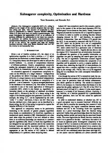
Let us consider the evaluation of a Kleene+ pattern under S3 . For ease of composition, we use a simplified version of Query 6, shown in Fig. 3(a), and a small event stream in Fig. 3(b). Each event is labeled with a letter specifying the pattern component satisfied, and the number for distinguishing it from other events of the same type. The events are also

listed with contained attributes. The NFAb model for this pattern is in Fig. 3(c). An initial set of operations according to the NFAb execution model are shown in Fig. 3(d). In the diagram, each box shows an operation in NFAb execution (the upper part) and the run after this operation (the lower part). We call such a diagram a “pattern execution plan”. To better explain it, we introduce the primitive operations based on the NFAb model: • Edge evaluation evaluates the condition on taking the transition marked by the edge, where the condition is compiled from the event type, time window constraint, and value predicates. • Run initialization is used to start a new run. • Run extension adds a new event to an existing run. • Run cloning duplicates an existing run to enable nondeterministic actions. • Run proceeding moves to the next automaton state without consuming events. • Run termination terminus a run when it arrives at the final state or it fails to find any possible transition. Then a pattern execution plan Γ is a tree of primitive operations, where each unique path in the tree is a run (ρ) of the NFAb . Next we state some key properties of this execution plan, which enable later optimization. First, we observe that S3 allows edge (predicate) evaluation operations to be postponed until later in the execution plan, which is a special type of “commutativity” allowed in the NFAb model. For instance, consider the evaluation of the ‘take’ edge in the NFAb in Fig. 3(c), where Kleene+ is trying to select more ‘b’ events. Let e denote the current event. The predicates in this edge evaluation are: e.type = B ∧ e.time < W ∧ e.val ≥ b[i − 1].val. If we postpone the value predicate, e.val ≥ b[i − 1].val, until the end of the plan, it is not hard to show that the plan still produces the same matches as before. Second, we observe that S3 also allows some suffix paths of the plan to be postponed altogether. To explain it, we introduce the concept of “consecutive operations”: Some of the primitive operations in the plan have to be performed consecutively. In Fig. 3(d), after step 1 is executed, step 2 must be performed immediately; otherwise this run will not be initialized and the following b1 will not be evaluated properly. We call such a pair of operations as consecutive operations (denoted by “↔”), meaning that other operations are not allowed between the two operations. In contrast, there are operations that do not need to be performed consecutively. This happens when a run is cloned in S3 . In Fig. 3(d), after step 3 finishes, due to the nondeterminism two actions are triggered: step 4 extends the current run with a new event, which needs to be performed right af-

PATTERN SEQ(A a, B+ b[], C c) WHERE [task_id] ^ b[i].val >= b[i-1].val WITHIN 100

Event time task_id val

(a) A simplified version of Q6 ignore

NFA >

begin

a

b[1]

begin

b1 4 6

b2 5 7

b3 6 9

c1 7 1 -

a1 b1

(b) An example event sequence

ignore

b[i]

a1 1 1 -

b2

ignore

proceed

c

begin

F

8.Run extension

take

...

b3

(a1,b1,b2,-)

(c) NFA^b for the query

1.Edge evaluation: a1 succeeds

2.Run initilization

3.Edge evaluation: b1 succeeds

-

(a1,-)

(a1,-)

Consecutive operations

...

4.Run extension


9.Run cloning

(a1,b1,-)

(a1,b1,-)

(a1,b1,-)

5.Run cloning


10.Run extension

(a1,-)

(a1,-)

(a1,b2,-)

...

Non-consecutive operations

11.Run cloning

(d) Pattern Execution Plan under skip till any match, for (a1, b1, b2, …)

(a1,-)

...

c1

NFA^b

Postponing

(a1,-)

(a1,-)

(a1,b1,-) (a1,-)

(a1,,-)

(a1,b1,b2,-) (a1,b1,-) (a1,b2,-) (a1,-) (a1,b1,b2,b3,-) (a1,b1,b2,-) (a1,b1,b3,-) (a1,b1,-) (a1,b2,b3,-) (a1,b2,-) (a1,b3,-) (a1,-) (a1,b1,b2,b3,c1) (a1,b2,b3,-) (a1,b1,b2,c1) (a1,b1,b2,-) (a1,b1,b3,c1) (a1,b1,b3,-) (a1,b1,c1) (a1,b1,-) (a1,b2,b3,c1) (a1,b1,b2,b3,-) (a1,b2,c1) (a1,b2,-) (a1,b3,c1) (a1,b3,-) (a1,-)

(a1,,-)

(a1,,-)

(a1,,c1) Then enumerate, (a1,b1,b2,b3,c1) (a1,b1,b2,c1) (a1,b1,b3,c1) (a1,b1,c1) (a1,b2,b3,c1) (a1,b2,c1) (a1,b3,c1)

(e) Runs w. and w.o. postponing

Figure 3: A running example for the postponing algorithm. ter step 3. In contrast, step 5 clones the current run to a new independent run for further processing, and thus even if it is not performed immediately, it will not affect the other run. We call a pair of primitive operations like steps 3 and 5 “non-consecutive operations” (denoted by →), e.g., 3 → 5, 6 → 9 and 7 → 11 in Fig. 3(d). In the plan Γ, all the pairs of non-consecutive operations allow us to decompose some suffix paths from the main path (which is highlighted in green in Fig. 3(d)). We denote the main path as ρ1 , and each suffix path as ρj = ρi +∆ρ, with some 1 ≤ i < j. The observations above lead to two propositions key to our optimization. The proofs are omitted due to space constraints. Proposition 5.1. Given a pattern execution plan Γ evaluated under S3 , if the run corresponding to the main path ρ1 is evaluated with value predicates removed, and if it produces an intermediate match, M = (ei1 , ei2 , . . . , eim ), then M is a superset of every match that can be produced by Γ. Proposition 5.2. Given a pattern execution plan Γ evaluated under S3 , the complete set of matches produced by Γ is the same as first obtaining the intermediate match M by running the main path ρ1 with value predicates postponed, and then enumerating all subsets of M while evaluating the postponed predicates. Postponing Algorithm. We now present the postponing algorithm that breaks the evaluation according to a plan Γ into two parts: pattern matching, which is shared by all of the original runs of Γ, and result construction. 1. Pattern matching. It follows directly from Proposition 5.1: we take the main run ρ1 and run it with all value predicates removed. This is the only cost incurred. 2. Result construction. This step follows directly from Proposition 5.2: We take the match M produced by the main run ρ1 with value predicates postponed. Then we enumerate all subsets of M while applying the postponed predicates, and return all the matches produced in this process. A simple optimization can be added to the enumeration process, e.g., ensuring that there is at least one event matching each pattern component in order to be a match.

Fig. 3(e) illustrates the postponing algorithm. Using the original plan, there are 15 runs. Using the postponing algorithm, there is only 1 run in pattern matching, producing an intermediate match M = (a1 , < b1 , b2 , b3 >, c1 ), and 7 cases in enumeration, leading to 7 final matches (in bold). Note that the benefits of the postponing algorithm are usually more than illustrated in this simple example: First, it can filter non-viable runs effectively. For example, a run that collects a large number of events for a Kleene+ component without finding an event for the last component is completely avoided in the postponing algorithm. Second, many fewer runs also mean the reduced evaluation cost for each event. Third, when a run reaches the result construction phase, the enumeration cost is still cheaper than the cost of cloning runs on the fly and repeated operations like edge evaluation on the same event can be carefully shared.

5.2

Postponing with Early Filters

A main drawback of the postponing algorithm is that the pattern matching phase removes value predicates and hence loses the ability to prune many irrelevant events early. To improve the filtering power, we would like to improve the postponing algorithm by performing edge evaluation, including the value predicates, on the fly as events arrive. However, it is incorrect to simply evaluate all predicates on the fly because it may not produce an intermediate match M that is a superset of every final match. Consider a Kleene+ on a sequence of values, (0.1, 0.2, 0.15, 0.19, 0.25), and two correct results for non-decreasing subsequences, (0.1, 0.2, 0.25) and (0.1, 0.15, 0.19, 0.25). If we evaluate the value predicate, b[i].val ≥ b[i − 1].val, in the main run ρ1 as events are scanned, we can produce an intermediate match M = (0.1, 0.2, 0.25), which is not a superset of (0.1, 0.15, 0.19, 0.25). Therefore, the decision on whether to evaluate a predicate on the fly should be based on its correctness, which is related to the consistency of evaluation results on a power set of an event sequence. Regarding consistency, we observe that all predicates applied to Kleene+ fall into one of four categories: True-value consistent predicates. A predicate in this category satisfies the following property: if the predicate

evaluation result of comparing the current event, e, against all selected events is true, then it is always true when comparing the event e against any subset of the selected events. Consider b[i].val > max(b[..i − 1].val) for Pattern(a, b+, c). If e.val is larger than the maximum of all selected events for the Kleene+, it will be larger than the maximum of any subset. So the “true” value is consistent. If an event fails the check, it is still possible to be larger than the maximum value of some subsets. So events validated by true-value consistent predicates on the fly do not need to be checked again in result construction; they can be labeled as “SAFE” to avoid redundant evaluation. Other events cannot be discarded and should be labeled as “UNSAFE” for additional evaluation in result construction. False-value consistent predicates. The property for this category is: if the predicate evaluation result of comparing e against all selected events is false, then it is always false for comparing e against any subset of selected events. c.val < max(b[..i].val) for Pattern(a, b+, c) is an example. Events evaluated to false by such predicates can be discarded immediately because they will never qualify. Other events must be kept for additional checking in result construction. True and false-value consistent predicates are predicates that are both true-value and false-value consistent predicates. An example is b[i].val > 5 for Pattern(a, b+,c). Since it does not compare b[i] with any of the selected events by Kleene+, the evaluation result will never vary with the subset of the events chosen. Events evaluated to true by true-false consistent predicates can be labeled as “SAFE”, and those evaluated to false can be discarded immediately. For this type of predicates, we can choose to directly output the intermediate matches of the pattern matching step as a collapsed format of the final results. This format includes all relevant events and provides a compact way to represent the final matches before enumerating them explicitly. The user may opt to pay the enumeration cost only when needed. Inconsistent predicates are predicates that are neither true-value consistent or false-value consistent. An example is b[i].val > avg(b[1..i−1].val) for Pattern(a, b+, c). This type of predicates should be postponed until result construction. With the knowledge of the four categories, the postponing algorithm can make a judicious decision on whether to perform predicate evaluation on the fly to filter events early.

5.3

Optimization on Confidence Computation

As mentioned in §4, there is an extra cost to compute the confidence of each pattern match in the presence of imprecise timestamps. This operation is prohibitively expensive for queries with Kleene closure, because the cost is exponential in the number of selected events. So we optimize it in this section. Our main idea is that existing work [30] finds all possible matches with confidence greater than zero. However, matches with low confidence are of little interest to the user. Setting a confidence threshold to prune such matches is of more value to the user, and it provides opportunities for optimization. The confidence of a partial match is non-increasing as more events are added to extend a partial match. In result construction, we can begin the enumeration with shorter runs (matches), and add events to validated matches one by one. If a shorter match has confidence lower than a threshold, then all longer matches with the same prefix will not need to be considered again. Based on this intuition, a dynamic programming method is

designed to optimize the performance of confidence computation, which reduces the cost drastically. Due to the limitation of space, the details are left to our tech report[31].

6.

EVALUATION

In this section, we evaluate our new system, called SASE ++ , with the proposed optimizations, and compare it with several state-of-the-art pattern evaluation systems.

6.1

Microbenchmarks

Queries in the microbenchmarks use the template, seq(A a, B+ b[ ], C c), unless stated otherwise, and S3 . We vary atches , two parameters: The selectivity (θ) defined as, #M #Events is controlled by changing the value predicates in the pattern. It is varied from 10−6 , which is close to the real selectivity in our case study, up to 1.6, which is a very heavy workload to test our optimizations. The other parameter is the time window (W ), varied from 25 to 105 . Our event generator creates synthetic streams where each event contains a set of attributes with pre-defined value ranges, and a timestamp assigned by an incremental counter or an uncertainty interval if the timestamp is imprecise. We run SASE ++ with the following settings: (1) Postponing, which applies postponing(§5.1) only; (2) On-thefly, which applies early filters (§5.2) based on postponing; (3) Collapsed, which returns results in collapsed format based on on-the-fly; (4) DP x: it applies dynamic programming (§5.3) with x% as the threshold based on on-the-fly. In addition to running SASE ++ with different optimization settings, we also compare it with (5) ZStream [20], which applies the optimization of placing a buffer of events at each NFA state and triggers pattern evaluation only when all the buffers become non-empty; (6) SASE+ [1, 28], which strictly follows the execution of the NFAb model, and (7) XSeq [21], which we describe in detail shortly. All experiment results were obtained on a server with an Intel Xeon Quad-core 2.83GHz CPU and 8GB memory. System SASE ++ runs on Java HotSpot 64-Bit Server VM.

6.2

Evaluation with Precise Timestamps

We first evaluate the two optimizations, postponing (§5.1) and on-the-fly (§5.2), using streams with precise timestamps. Throughput. Figure 4(a)-4(b) show the throughput while varying θ and W for the true-value consistent predicates. The y-axis is in logarithmic scale. We see that the throughput of SASE+ drops very fast as θ and W increase. ZStream’s performance degrades similar to SASE+. Our postponing algorithm works well; its performance goes down only slightly. On-the-fly has a similar performance as postponing in this workload. Figure 4(c) shows the number of runs created with varied W . The plot confirms our runtime analysis that the numbers of runs in SASE+ and ZStream can go up exponentially and thus their throughput drops quickly. In contrast, the number of runs in postponing algorithm increases much more gradually. We further show the throughput when varying W for the false-value consistent predicates in Figure 4(d). Here, onthe-fly performs better than postponing because it can discard more events earlier when evaluating them on the fly. Results for the other types of predicates are omitted because they exhibit similar trends as shown in these plots. Cost breakdown. We further break down the cost of each system by profiling time spent on each operation. The

1e+05 1e+04

On-the-fly Postponing ZStream SASE+

1e+03 100 0.0035

0.5

1

1.5

1e+07

1e+06

Number of runs

Throughput (events/second)


1e+06

1e+06

On-the-fly 1e+05 Postponing ZStream SASE+ 1e+04 1e+04

Selectivity(matches/event)

5e+04

On-the-fly Postponing ZStream 1e+05 SASE+ 1e+04 1e+03 100 1e+04

1e+05

Time window (time units)

(a) Vary θ (T-value consistent predicates)

5e+04

1e+05

Time window(time units)

(b) Vary W (T-value consistent predicates)

(c) Number of runs with varied W (T-value

1e+06

On-the-fly 1e+05 Postponing

ZStream SASE+

1e+04 1e+04

5e+04

1e+05

1e+09 1e+08 1e+07

Total Pattern Matching Run Initialization

1e+06 1e+05 1e+04


(d) Vary W (F-value consistent predicates)

Time cost (microseconds)



consistent predicates) 1e+07

5e+04

1e+05

1e+09 1e+08 1e+07

1e+05 1e+04


(e) SASE+ cost breakdown with varied θ (T-value consistent predicates)

Total Run Initialization Result Construction Pattern Matching

1e+06

5e+04

1e+05


(f) On-the-fly cost breakdown with varied θ (T-value consistent predicates)

Figure 4: Microbenchmarks results with precise timestamps breakdown of SASE+ is shown in Figure 4(e). The run initialization cost stays the same because only events qualified for the first component trigger this operation and the same stream is used. The rest of the cost is attributed to pattern matching, which is exponential in W . The cost breakdown for the postponing algorithm with predicate evaluation onthe-fly is shown in Figure 4(f). Using the run initialization as a reference, the cost for pattern matching stays low all the time. The cost for result construction increases because runs tend to collect more events as W increases. However, it is still lower than the run initialization cost for most time. Summary. Overall the postponing algorithm can provide up to 2 orders of magnitude improvement (max. 383x) over SASE+ and ZStream. The pattern matching phase can reduce the cost from exponential to polynomial, and sometimes close-to-linear cost. Although the result construction phase may still generate an exponential number of matches, which are determined by the query, the cost is much smaller than SASE+ and ZStream, and returning them in a collapsed format is an option for further reduction of the cost.

6.3

Evaluation with Imprecise Timestamps

In this set of experiments, we generate streams where each event has an uncertainty interval size of 10. Fig. 5(a) shows the throughput for varying W with true-false value consistent predicates. The postponing algorithm without dynamic programming optimization is dominated by the cost of confidence computation, which is highly sensitive to W . It fails to run when W > 3000, which is too small for practical uses. The dynamic programming (DP) optimization can support larger windows and improve performance as the confidence threshold increases. The collapsed format returns results in a compact way, without enumerating all the matches, hence setting the upper bound of performance. The cost on confidence computation for different algorithms is as shown in

Fig. 5(b). Note that the DP method is based on the postponing algorithm; without the intermediate matches, such optimization on confidence computation is not feasible.

6.4

Comparison with XSeq

We further compare the performance of our system with XSeq, an engine for high-performance complex event processing over hierarchical data like XML, JSON etc. For comparison, the same synthetic stream is used, and it is converted to the SAX format required by XSeq. Since we use S3 , XSeq is set to the All Match Skip One mode, which finds all possible matches for each starting point. The optimization method of XSeq is set to VP OPS OPTIMIZATION, which gives the best performance. We first vary the query length l for seq(A1 , . . . , Al ). The result is in Fig. 5(c). A line marked by “XSeq n” means that the input includes n events. XSeq is sensitive to the input size so it does not scale well, while our system is stable with the input size and its throughput is about 4 to 10 orders of magnitude higher. Then we compare to XSeq by varying time window W for the usual Kleene+ pattern, which is shown in Fig. 5(d). The throughput of XSeq is still much lower and sensitive to the input size. We observe the performance of XSeq is always low and not affected by W . A main observation is that XSeq is not optimized for the time window. For example, if the query is, seq(a, b) within 25, XSeq will compare every a with every b in the input, instead of terminating when no future events can fall into the time window. This can be a straightforward optimization but we were given only a binary executable of XSeq without the source code. Second, XSeq is optimized for different selection strategies. Among 13 sample queries with Kleene closure in the paper [21], 5 queries are applied to children of nodes, the depth of which can be limited; the other 8 queries are applied to on immediate following siblings, and this is

1e+05 1e+04 1e+03

Collapsed DP 0.999 DP 0.99 DP 0.9 DP 0.7 On-the-fly SASE+

100 10 1e+04

5e+04

1e+05

1.5e+05

1e+10 1e+09 1e+08 DP 0.999 DP 0.99 DP 0.7 SASE+

1e+07 1e+06 1e+05 1e+04

2e+05


5e+04

1e+05

1.5e+05

1

(b) Cost on confidence computation with imprecise timestamps

0.001 2

1e+03

10 25

50

75

100

80% 60% 40% 20%

25

15 10 5

Time range (seconds)

0 0

1000

2000

3000

4000

Time since the job started (seconds)

(g) Data queuing in Worldcup U

(f) Data queuing in the Twitter job

1e+08

Throughput(events/second)

40

500 1000 1500 2000 2500 3000 3500

Time since the job started (seconds)

(e) Mapper average running time Throughput(log, events/second)

Worldcup U 80

0

(0,10] (10,20] (20,30] (30,40] (40,50] (50,60] (60,70] (70,80]


120

Twitter

20

0 0

(d) XSeq for a Pattern(A,B+,C), varied W

5

30 WorldCup U WorldCup S Twitter

0 10

4

(c) XSeq for a pattern(A1 ,. . .,Al ), W =25 Queuing data size (GB)

On-the-fly XSeq 10 XSeq 30

3

Query length

100%

Accumulative percentage

1e+07

1e+05

On-the-fly XSeq 10 XSeq 30 XSeq 100 XSeq 300

2e+05

with imprecise timestamps Throughput (events/second)

1e+03


(a) Vary W , TF-value consistent predicates

Queuing data size (MB)

1e+06


1e+11



1e+06

1e+07 1e+06 100000 10000 1000 100 10 1

1e+08 Postponing 1e+07

On-the-fly DP 0.999

1e+06 1e+05 1e+04 1e+03 100 10 1

Q1

Q2

Q3

Q4

Q5

Q6

(h) Throughput for all queries

Q5

Q6

(i) Optimizations

Figure 5: Results for imprecise timestamps, comparison with XSeq, and Hadoop use case study like S1 . XSeq lacks optimizations for more flexible selection strategies, S2 or S3 . Overall, XSeq is not optimized for the ability to “skip” events, which is one of the core features of CEP. It is largely due to the fact that XSeq is designed for processing hierarchical data instead of general event streams.

6.5

Case study: Hadoop Cluster Monitoring

As stated in recent work [22], Hadoop cluster monitoring is still in its adolescence. By working with Hadoop experts, we perform a detailed case study to demonstrate that our system can help automate cluster monitoring using declarative pattern queries and provide real-time performance. Data collection. We collect two types of logs in realtime: the logs of system metrics, e.g., CPU usage, network activity, etc, and the logs of Hadoop jobs, e.g., when a job starts and ends. Ganglia [18], a popular distributed system monitor tool, is used as the core part of our real-time data collection system. We use gmond, which is the monitoring daemon in Ganglia on every node, to grab performance metrics from the OS, and we also customize it to parse Hadoop logs. Gmeta is the polling daemon, which polls logs and saves to round-ronbin databases (RRD). Then our system reads the data for pattern evaluation. Queries. We develop 6 queries together with Hadoop ex-

perts to analyze Hadoop performance. They all use Kleene+ patterns and some use uncertainty intervals. As Q1 and Q6 are already shown in Table 1, we discuss other queries below. Recall that Q1 computes the statistics of lifetime of mappers in Hadoop. Similarly, Q2 does it for reducers. Fig. 5(e) shows the average lifetime of mappers for three different workloads : Twitter (raw data 53.5GB, map output 565GB), which counts statistics for tri-grams from tweets; Worldcup U (raw data 252.9GB, map output 32GB) analyzes the frequent users from the logs for clicks on 1998 FIFA Worldcup website; Worldcup S (raw data 252.9GB, map output 263.5GB), divides user clicks into sessions. In the figure, the Twitter job has much longer running time than the other two workloads because the output size of its mappers is larger. Q3 is used to find the data pull stragglers. A reducer is considered as a straggler when its runtime is two times the average of other reducers [22]. Given the task id returned by the query, user can then check logs and locate the specific information to know what was wrong with that task. Q4 offers real-time monitoring for the queuing data size. As mappers output intermediate results, reducers may not consume them immediately, which leads to data queuing. The data queuing in the lifetime of Twitter workload is shown in Fig. 5(f). The first peak implies that most map-

pers have completed their tasks; then the queuing size starts to reduce as data is consumed by reducers. Fig. 5(g) is the queuing size for the Worldcup U workload which is different. The job has not really started until 2300 seconds passed. This is because concurrent jobs are running and it has to wait. Our Hadoop experts find these results very helpful. Q5 and Q6 are used to find tasks that cause cluster imbalance. As Q6 is described above, we simply note that they both use uncertainty intervals for timestamps due to granularity mismatch of Ganglia logs and Hadoop logs, and differ only in the ways of defining imbalanced load. Performance. Fig. 5(h) shows throughput of all 6 queries, ranging from 300,000 to over 7 million events per second. The data rate in our experiment is 13.62 event/second/node. This means that a single server running system SASE ++ can monitor up to 22,000 nodes in real-time for these queries. For post analysis, it only takes 0.00454% of the actual running time of the monitoring process. Authors of [22] provide some public datasets, where the data rate is 0.758 event/second/node in the busiest month. Fig. 5(i) compares the optimization algorithms for Q5 and Q6. More results are available in our tech report [31].

7.

RELATED WORK

CEP languages. In §3 we analyzed and compared a large number of CEP languages with different descriptive complexity. Other languages such as TESLA [10] do not introduce new features beyond those surveyed languages. Temporal models. The discussion for CEP with imprecise timestamps is based on recent work on supporting an uncertain temporal model [30]. However, this work neither supports Kleene+ queries nor has optimization for confidence computation. The performance of [30], with an extension for Kleene+, is shown by the blue line in Figure 5(a), which is too slow for Kleene+. In contrast, our dynamic programming optimization enables early pruning of matches with low confidence, which improves performance significantly (as shown in the above-mentioned figure) and makes Kleene+ queries under the uncertain temporal model fast enough for practical use. Other temporal models [3, 2, 6, 11] use time intervals to represent precise event durations, instead of uncertain occurrence time, and hence do not address uncertainty in pattern matching and related complexity. Optimizing CEP performance. Improving the performance of CEP queries has been a focus of many works. Recent studies make use of sharing among similar queries to reduce cost [15, 29]; optimize for performance given out of order streams [13]; optimize the performance of nested pattern queries by pushing negation into inner subexpressions [16]; and rewrite queries in a more efficient form before translating them into automata [24]. In distributed systems, the work [2] applies plan-based techniques to minimize event transmission costs and efficiently perform CEP queries across distributed event sources.

8.

CONCLUSIONS

This paper presented theoretical results on expressive power and computational complexity of pattern query languages in CEP. These results offer insights for developing three optimization techniques. Comparison with existing systems shows the efficiency and effectiveness of a new system using these optimizations. A thorough case study on Hadoop cluster monitoring also demonstrates its practical value. In future work, we will consider ways to integrate with approxi-

mate pattern matching when events carry uncertain values.

9.

REFERENCES

[1] J. Agrawal, Y. Diao, et al. Efficient pattern matching over event streams. In SIGMOD, 147–160, 2008. [2] M. Akdere, et al. Plan-based complex event detection across distributed sources. PVLDB, 1(1):66–77, 2008. [3] M. H. Ali, C. Gerea, et al. Microsoft cep server and online behavioral targeting. VLDB, 2(2):1558–1561, 2009. [4] R. Alur and P. Madhusudan. Visibly pushdown languages. In STOC, 202–211, 2004. [5] A. Arasu, S. Babu, et al. The CQL continuous query language: semantic foundations and query execution. VLDB J., 15(2):121–142, 2006. [6] R. S. Barga, J. Goldstein, et al. Consistent streaming through time: A vision for event stream processing. In CIDR, 363–374, 2007. [7] D. A. M. Barrington, N. Immerman, et al. On uniformity within nc1 . J. Comput. Syst. Sci., 41(3):274–306, 1990. [8] J. Boulon, A. Konwinski, et al. Chukwa, a large-scale monitoring system. In CCA, volume 8, 2008. [9] Z. Cao, C. Sutton, et al. Distributed inference and query processing for rfid tracking and monitoring. PVLDB, 4(5):326–337, 2011. [10] G. Cugola and A. Margara. Tesla: a formally defined event specification language. In DEBS, 50–61, 2010. [11] A. J. Demers, J. Gehrke, et al. Cayuga: A general purpose event monitoring system. In CIDR, 412–422, 2007. [12] N. Immerman. Descriptive Complexity (Texts in Computer Science). Springer, 1999 edition, 1 1999. [13] T. Johnson, et al. Monitoring regular expressions on out-of-order streams. In ICDE, 1315-1319, 2007. [14] J. Kamp. Tense logic and the theory of linear order. 1968. [15] S. Krishnamurthy, C. Wu, et al. On-the-fly sharing for streamed aggregation. In SIGMOD, 623–634, 2006. [16] M. Liu, et al. High-performance nested cep query processing over event streams. In ICDE, 123–134, 2011. [17] D. Luckham. Event Processing for Business: Organizing the Real-Time Enterprise. Wiley, 2011. [18] M. Massie, B. Li, et al. Monitoring with ganglia, 2012. [19] R. McNaughton and S. A. Papert. Counter-Free Automata (MIT research monograph no. 65). The MIT Press, 1971. [20] Y. Mei and S. Madden. Zstream: a cost-based query processor for adaptively detecting composite events. In SIGMOD, 193–206, 2009. [21] B. Mozafari, et al. High-performance complex event processing over xml streams. In SIGMOD, 253–264, 2012. [22] K. Ren, Y. Kwon, et al. Hadoop’s adolescence. PVLDB, 6(10):853–864, 2013. [23] R. Sadri, C. Zaniolo, et al. Expressing and optimizing sequence queries in database systems. ACM TODS, 29(2):282–318, 2004. [24] N. P. Schultz-Møller, et al. Distributed complex event processing with query rewriting. In DEBS, 4. , 2009. [25] H. Vollmer. Introduction to circuit complexity: a uniform approach. Springer, 1999. [26] D. Wang, et al. Active complex event processing over event streams. PVLDB, 4(10):634–645, 2011. [27] D. Wang, E. A. Rundensteiner, et al. Probabilistic inference of object identifications for event stream analytics. In EDBT, 513–524, 2013. [28] E. Wu, Y. Diao, et al. High-performance complex event processing over streams. In SIGMOD, 407–418, 2006. [29] D. Yang, E. A. Rundensteiner, et al. A shared execution strategy for multiple pattern mining requests over streaming data. PVLDB, 2(1):874–885, 2009. [30] H. Zhang, Y. Diao, et al. Recognizing patterns in streams with imprecise timestamps. PVLDB, 3(1):244–255, 2010. [31] H. Zhang, et al. Optimizing expensive queries in complex event processing. Tech Report, http://sase.cs.umass.edu/.