Aug 15, 1988 - For the 357,000 acre (1,500 km2) Columbus Metropolitan Area, the ... system, the city decided to develop a SWMM model to simulate the ...
Chapter 8 - - - - - - - - - - -
On the Optimization of Uncertainty, Complexity and Cost for Modeling Combined Sewer Systems
William James, Taymour El-Hosseiny aad Hagh. R Whiteley
This chapter introduces a tentative procedure for estimating the minimwn level of complexity of a computational model for designing a cost-effective combined sewer overflow (CSO) system. In this approach, model complexity is related to a measure of model uncertainty, and to the design costs. Ultimately the goal is to determine the optimal (least cost) complexity for a model (version 4.3 of the U.S. EPA Storm Water Management Model, SWMM) which is itself uncertain. Differences between modelers, and errors in datafiles could invalidate our proposed method. Thus we propose a procedure that first produces consistent models free of user-input error. Developed in the form of an expert system shell, our procedure uses a front-end rule-based (FERB) decision support system (DSS). This FERB-DSS comprises two functions, model development, and sensitivity analysis: first the user is led through the development of consistent input files; second a heuristic sensitivity analysis procedure is applied to selected model parameters. In a following step, calibrated parameters that consistently reproduce observations are determined. Finally, minimum uncertainty and corresponding cost production functions are derived, and from these parameters an optimal level of model complexity is defined. This chapter describes the final step, as well as the problem of determining a globally optimum set of calibration parameters for SWMM. James, W., T. El-Hosseiny and H.R. Whiteley. 1998. "On the Optimization of Uncertainty, Complexity and Cost for Modeling Combined Sewer Systems." Journal of Water Management Modeling R200-08. doi: 10.14796/JWMM.R200-08. © CH11998 www.chijoumal.org ISSN: 2292-6062 (Formerly in Advances in Modeling the Management ofStormwater Impacts. ISBN: 0-9697422-8-2)
135
136
Optimal Uncertainty and Complexity ofModels
Using 1994 U.S. EPA policy as a guideline for design, our proposed method is applied to a complex and costly problem: CSO controls in Columbus OH. We conclude that analysis of uncertainty is essential when using models to design CSO controls.
8. I Introduction Engineering designs of stormwater and wastewater drainage systems are clearly becoming increasingly complex. Nowadays their objectives are to minimize problems caused by water drainage, to meet expanded and strengthened water quality standards, and to protect both public health and aquatic life. Many of the problems to be corrected are related to wet weather performance of these drainage systems. Wet weather problems may be obvious and recorded, like basement flooding and flooded roads, which result in health hazards, loss of local property values, and sometimes, loss of property. Or they may go unrecorded, despite their serious consequences. For example, when a sanitary sewerage system surcharges (hydraulic grade line rises above the sewer crown), due perhaps to a constriction downstream, suspended solids may deposit in the conduit network, reducing cross-section and capacity. Intensive monitoring studies are rarely feasible in these cases, due to cost and the delay. On the other hand, computational drainage models are valuable tools for assessing drainage system response to various wet weather events, especially when evaluating alternative control strategies (WEF, 1994). Models can be tested against real or synthetic events, and input parameters can be optimized and verified against observations or against other design criteria. Once verified, a model may be used with an appropriate level ofcertainty for simulating unmonitored conditions, for design optimization of the sewerage system and for real-time control. To solve even the identified problems, the first step of selecting the best modeling options is itself problematic. Concerns include: • What array of models should be used? • What is the extent of model applicability in the context of the study objectives? • What level of design accuracy is achievable? • What is the uncertainty of the model results? • What investment of modeling effort is most cost-efficient? • Is cost-efficiency an appropriate measure for optimi zing an uncertain design? Such questions beg the issue of model complexity, which affects the requirements for data collection, the model calibration effort, selection of the objective function (e.g. total flow, peak flow, duration of flow exceedance), and
8.2 Procedure for Determining Optimal Complexity
137
selection of modeling options. Extremes of model complexity may lead to the user becoming mired in small details of process disaggregation, system discretization and model reliability, or so siniplifying the modeling process that the exercise results in over- or under-, design. One approach to this optimmltion problem is to perform detailed sensitivity and error analyses ofthe models, based on specific criteria (e.g. weighted error). However, computational resources required for complex, continuous hydrologic models (e.g. simulation of75 years of data) still present a problem, whether real or imaginary. Spectres of nonlinearity and global optimimtion are inevitably raised, and are addressed later. To demonstrate our approach, the SWMM model (Huber and Dickinson, 1988)wasusedinourstudy.SWMMsimulatesmanyaspectsofurbanhydrology and hydraulics including surface runoff and pollutant routing through a water channel or a collection system. Obviously, for reliable, efficient use, a complete understanding ofthe model and its limitations is required. 8utforthe average user the SWMM interface presents a barrier, and care and attention is necessary. There is a clear role for intelligent interfaces such as PCSWMM97 (James and James, 1998). In our study we introduced a method for interfacing SWMM with a knowledge base, and applied an error analysis to evaluate the credibility of the resulting model. Two general objectives were: 1. develop a FERB-DSS to interface with SWMM, and 2. optimize the modeling effort against model uncertainty using a systematic cost-effectiveness procedure (in other words, estimate the optimum value of model complexity considering reliability of model results and design costs). In this chapter we do not cover the first objective, but focus on the latter objective.
8.2 Procedure for Determining Optimal Complexity Cost estimation factors that make each case study unique include: level of risk acceptable to a community; number of sensitive areas (outstanding national resources, national marine sanctuaries, water that provides habitat for endangered species, waters with primary contact recreation, and water used for public water supply and shell fish); and 3. savings due to the management of damages. Ultimately a relationship is required between system cost and model uncertainty, which can be further processed to produce the minimum cost. Cost is taken to be a combination of the following: 1. 2.
Optimal Uncertainty and Complexity ofModels .
138
1. 2. 3. 4.
engineering fees to design alternative solutions; construction costs of the selected alternative; intangible costs; damage costs due to uncertainty of the selected option. Figure 8.1, not drawn to scale, depicts these relationships for a costeffective design using arbitrary units. Total combined cost of the selected alternative is the sum of the individual unit cost at pre-defmed levels of uncertainty. The cost-effective design is taken to be least-cost combination. Design costs can be estimated as a function of model components. Construction costs can be estimated as a function of design flow rates or storage volume, and rise with uncertainty, because of the tendency to over-design as uncertainty increases. Uncertainty cost arises from a failure of the design to achieve the correct optimum size thus incurring either excessive construction costs or excessive environmental and other intangible costs. However, assigning a dollar value to intangible costs is difficult due to its wide variation. Thus an index value was assigned to the intangible cost based on a weighting factor and the uncertainty. Ifwe ignore intangible costs in the total costs, capital costs will likely control the EF, because the design costs are a small percent of the total. If intangible costs are included, total cost can be expected to reach a minimum (optimal) value at a certain level of complexity.
0.2
0.4
0.6
0.8
1.2
1.4
Uocertaillly
Figure 8.1 Cost optimization of CSO control option (arbitrary units).
Our proposed method may be said to derive the components schematized in Figure 8.1, and we tentatively proposed a procedure in point form as follows: • Formulate all possible processes (e.g. snow melt, infiltration, run-off, storage) to be modeled and the associated parameters and variables. • Estimate initial values for the model parameters. • Select an objective function (OF) that serves the objectives of the
8.3 Application to Columbus, Ohio
• •
• •
139
analysis. Here our objective is to determine a cost-effective model to design a CSO control facility, which is often related to storage volume, so we selected total runoff volume as the OF for the uncertainty analysis. Select a state-variable (SV) for input (e.g., high, medium, low rainfall intensity) and run the model. Apply a first-order sensitivity analysis to determine the sensitivity of model parameters selected for that SV, based on literature reviews and prior experience. Repeat steps 3 and 4 for all input SVs. Evaluate results from the sensitivity analysis and deactivate unnec-
essary processes.
• • •
• •
•
• •
Compare model results to observed data (total volume of each runoffhydrograph) and determine the error in computing the OF. Select an error function (EF) as a measure of uncertainty. We used the first dimensionless form of the simple least square equation because it favors large flows. Calibrate model results to minimize differences between observed and computed OF based on sensitivity of model parameters. Sequentially assign more or less complexity (i.e., increase or decrease the number of modeled sub-spaces, watersheds or pipes) and estimate the error in the OF at each level of complexity. Calculate total costs of a control measure ofCSO's using the U.S. EPA policy guidelines. Using model results at each level of complexity, the control facility is redesigned. Total costs are the sum of monetary, intangible costs and uncertainty costs. The monetary costs are the construction and engineering fees. Intangible costs are assumed to be an inverse function of the size of the control facility. Uncertainty costs are constructed from weighted functions for the extra cost due to deviation from the minimum optimal size as a result of model uncertainty. Add design office costs. Produce a relationship between total cost and model complexity. Estimate a reasonable level of complexity for minimum cost
8.3 Application to Columbus, Ohio For the 357,000 acre (1,500 km2) Columbus Metropolitan Area, the Division of Sewerage and Drainage (DOSD), collects, transports and treats sanitary wastewater and stormwater flows. In the center ofthe city, the combined sewer shed (CSS) area has been divided into sanitary sewer-sheds (SSs) and
140
Optimal Uncertainty and Complexity ofModels
runoff catchments (RCs), whose total area is about 5,285 acres (22 km2), about 1.5% ofthe current and future service area. They drain from east to west and flow in the main interceptor (OSIS) sewer that travels from north to south, parallel to the Olentangy River, where the river merges with the Scioto River. OSIS was planned to carry sewage from the combined sewer area in the central portion of the city and the outlying county sewer districts, which are served by separate sanitary sewer systems. It was designed in 1930 for a 3D-year design period to serve a tributary area of 55,424 acres (232 km2), with estimated average DWF of 125 U.S. gal!capita.day (468 Llcapita.day). Included was a provision for control of storm-sewage entering from the combined sewers via nineteen regulator chambers at the connections of the combined sewers and OSIS, designed to overflow during flows that exceed the capacity of OSIS. An adjustable sluice gate is installed at each regulator chamber to control the amount of flow entering OSIS. OSIS was designed such that the combined sewers would overflow an average of eight times per year. A stand-by tank was constructed at the end of OSIS and upstream of the POTW to provide partial treatment ofthe excess storm sewage flow. Nearly 30 years after the end of the design period, during the 1980's, officials realized that the original design assumptions for many of the existing interceptor sewers no longer held. Current conditions were highly dynamic, unknown sources of excessive inflow and infiltration were present in the combined system, and water backed up into basements. The frequency of overflows from the combined sewer system was unknown. According to U.S. EPA requirements for long-term control plans for combined sewer systems, each municipality should adopt either the presumption or the demonstration approach. The presumption approach requires that the maximum number of overflows should not exceed four per year. A review ofdesign reports for the CSS revealed that the north side of the central area of the City of Columbus was designed for eight overflows per year. Because ofthe complexity ofthe collection system, the city decided to develop a SWMM model to simulate the collection system and investigate its response to various hydrologic factors.
8.3.1 Discretization of sanitary sewer-sheds and runoff catchments SWMM RUNOFF was used to generate runoff hydrographs at each RC. EXTRAN was used to route computed flows through the collection system. Table 8.1 summarizes all tasks related to each RC.
8.3.2 Monitoring Program Monitoring was carried out for the study area by URS (1989). Their program included installation of a rain gage network and flow monitors. A flow monitor was installed at the end of each tributary area and upstream of its
8.3 Application to Columbus, Ohio
141
Table 8.1 Runoff catchment data extraction task. 1.
2.
Interceptor Level: Develop covering maps for combined sewer system IdentitY modeled sewers Get record drawings fur modeled sewers Generate Pipe Ambiguity Record to clarity linkage IdentitY modeled storm sewers IdentitY interceptor sewer IdentitY sewers and areas discharging to separate storm system Get topographic maps CatcbmentLeveI: Transfer modeled nodes from sewer-shed bw;e Delineate outer catcbment boundaries Identity new nodes required for modeled sewers
3.
Subcatcbment Level:
Complete interior boundaries using small diameter sewers IdentitY nodes fur subcatcbment contribution Extract the following parameters fur subcatcbment Areas
4.
Width Percent Imperviousness (1KlriaI photography) Ground slopes (average along overJand flow) Modeled Sewers: IdentitY nodes using record drawing profiles Extract new or revised sewer segments using die identified nodes
regulator. Data were recorded at IS-minute intervals. and included simultaneous water depth and velocity. A rain gage network of20 rain gages was constructed to monitor rainfall time series across the entire City ofColumbus area. Rain gages consist of a computer as a data logger and a tipping bucket measuring 0.01 inch (0.25 mm) per tip. 8.3.3 Summary of Precipitation Observations:
A frequency analysis of rainfall data was carried out to determine (i) different levels ofSVs for modeling purposes, and (ii) the relationship between rainfall and overflow frequency. This analysis used data collected between 1988-1994 for rain gage 14. Precipitation events were separated using a minimum inter-event time (MIT) of4 hr based on a qualitative analysis using different values of MIT of from 3 to 7 hr (EMH&T, 1994). The MIT is an artificiallychosen minimum number of consecutive zero precipitation hours separating two storm events. Storms varied in intensity from 0.1 in. (2.5mm) per day to 4.25 in. (106 mm) per day, but only storms above 0.2 in. (5 mm) per day were considered in this study. A total of357 events were ranked, based on total rain, for years 1988-1994.
Optimal Uncertainty and Complexity ofModels
142
After reviewing the flow data, the recorded daily precipitation were classified into three state variable (SV) spaces: sv Space
Rainfall Total (x)
Small
0.2 25 mm)
The model was tested and calibrated against aU SVs (Le., small, moderate and large events) based on the above criteria for total rainfall. From the entire precipitation record, five representative events were then selected.
8.3.4 Model Development: Major tasks of the modeling procedure were: Develop a database that manages discretized data customized to fit the requirements of the selected model. 2. Select flow component(s) needs to be analyzed (e.g., DWF, base infiltration). 3. Identify special modeling concern based on API (e.g., diversion chamber, boundary condition. overflows, and storage). 4. Develop two model runs, one for DWF using SWMM TRANSPORT and another for rainfall-runoff using SWMM RUNOFF. S. If tributary SS is modeled for wet conditions, develop Infiltration! Inflow (III) based on flow monitoring data to define rainfall dependent infiltration/inflow (RDn). III hydrographs are stored at predefined nodes within SWMM TRANSPORT. 6. Combine aU flows at common nodes (Le. DWF, RlIDoff, III). 7. Route combined flows using SWMM EXTRAN and assign valid boundary conditions. 8. Compare model results with observed data at selected nodes and conduits for a predefined OF. For first OF chosen was peak flow to assess capacity of the collection system. The second was overflow volume and its frequency, chosen to meet U.S. EPA policy. 9. Carry out sensitivity analyses for selected parameters to assist in model calibrations. 10. Estimate errors in the OFs. 11. Determine optimum estimates of model parameters and rerun the modeL 12 Repeat steps 10 and 11 until differences between computed and observed OF become constant and no improvements occur in estimated error. 13. Display model results. 1.
8.3 Application to Columbus, Ohio
143
8.3.5 Model Development and Calibration: The total acreage of SS is about 600 acres and of RC is about 270 acres, almost fully developed. The primary activities within each subcatchments are categorized as follows: single-family residential, multi-family residential, commercial, industrial, and open areas. To optimize model resolution (i.e. optimum number of RCs and SSs, and optimum number of calibration trials). three datasets: 27, 10 and 1 RCs, were set up. Figure 8.2 is the schematic for 27 RCs. Initial model parameters were discretized based on 27 local areas. Aggregation of model parameters was based on parameter type. For example the area parameter was aggregated by the summation of local RC and SS, percent of imperviousness was aggregated using the following equation: %impi
L (%impi x Areaj) L (Areaj)
(8.1)
where: %imPi %impj are~
= =
% imperviousness of aggregated area i % imperviousness of local area j total acreage of area j
Width of the RC was based on the longest path offlow at each RC. Ground slope was recalculated based on average ground slopes after aggregation. 8.3.6 SensitMty Analysis:
Sensitivity coefficients were derived to generate a sensitivity matrix that can be used in model calibration and error analysis, in an order that distinguishes between the orders of confidence in the estimated input values: Order 1: Parameter can be estimated with an expected size of error between 1-1 0% (e.g., diameter, pipe length, pipe slope). Order 2: Parameter can be estimated with an expected size of error between 10-20010 (e.g., flow, ground slope, ground elevation). Order 3: Parameter with an expected size of error between 20-30% (e.g., infiltration parameters, pipe roughness). Order 4: Parameter with an expected size of error between 30-100% error (e.g., initial soil-water deficit). Order 5: Parameter cannot be measured and no level of confidence can be assumed (e.g. % imperviousness, depression storage subcatchment width).
....... ,j::o. ,j::o.
LEGEND:
> (ffi) 6
~
o
Overllow flow Divider Regulator Chamber LOCI I Area
Point Source (Manhole)
~ §.
a ~
~
is'
~.
~ g ~...,
~ ~
~ ~ Figure 8.2 Schematic of Tributary areas to Frambes St regulator, using 27 local areas.
~
~
1;;"
8.3 Application to Columbus, Ohio
145
Dunn and James (1985) recommended at least three values for each parameter to account for the expected range and distribution of estimates of parameters. Their approach indicates whether computed results are approximately linear or nonlinear, so that an appropriate sensitivity analysis method may be applied. Sensitivity analysis was applied twice, once for a complex model with 27 RCs and SSs, and another for a less complex model with ten RCs and SSs. No sensitivity analysis was carried out for one RC due to its obliviousness of relief structures upstream of the last node. Sensitivity gradients were obtained for the following six parameters, which can be considered to be the least-confident parameters that influence the OF (peakflow or overflow volumes) (James and Robinson, 1981) and (Zaghloul, 1983): area, percent of imperviousness, ground slope, runoff catchment width, impervious depression storage, pervious depression storage. Peak. flow was used as an OF to display sensitivity. James and Robinson (1981), Zaghloul (1983), and Lei and Schilling (1993) applied sensitivity analysis for the above parameters and showed that the sensitivity gradients for peak flow as an objective function yields the same gradients as for flow volume. In this study, peakflow was used as the OF for the sensitivity analysis butflow volume was used for the design of the CSO control facility. Dominant parameters were selected based on their sensitivity: area, % of imperviousness, subcatchment width. Sensitivity gradients were computed using normalized (relative) sensitivity so that comparisons can be made irrespective of parameter units:
(8.2)
where: ~
o p
=
relative sensitivity output objective function input parameters
The analysis showed that peak. flow sensitivity increased with complexity (higher number ofRes ). The relative sensitivity 1\, using percent ofimperviousness as indicator decreased by 17% by increasing model complexity from 10 RCs to 27 RCs. The impact was higher using subcatchment width as indicator, where ~ decreased by 50%. Figures 8.3 and 8.4 illustrate sensitivity gradients for different complexities and the following percent chances of the parameters around its mean value: +/20%, +/-50%, and +/-70%. Results of sensitivity gradients for percent of imperviousness showed that as complexity (number ofsubcatchments) increases, a decrease in sensitivity occurs using % imperviousness and subcatchment width as indicators.
Optimal Uncertainty and Complexity ofModels
146
~r-~--~--~~--'-~--~-,
,I I. ~ ~ _"',1, ... r' . , j"l-'I";" I ,\ ' . I iIi.
~
,.,
iQ. ""'
-"'' ' 1'
.'1 "1,'... .
I i i~
r
1
I
1
Elml--+-+--+-+--+-+--+--I
~
,I
'; .- - ..·l ... ·r···
; •i.' !
Cl
I
i.
..1.-.1 .
• .
i__ I __
~\L-~
.RO'I.
~
..(aQ%
..am
~~
.20%
i
I
I .
1
I ! I i '"!." ._..... I: •. ~.~~.I,I"'.... ~. j ! i
..c lO\1• _..·· ..·'1'·i ....·· t'.1··.. ··· .~"•. ' U' ;f!.
1..........
i
__
M.
~~
2Cn~
__
...,,\
-b~
60%
W.
Ofo Change in Imperviousness Figure 8.3 Impact of% imperviousness change on computed peak flow.
,
. 1 r--r--T' " tnv. .'. .'+'--.. ~;.-
;.. .1... , j
~L-~
__
__
.w"
~
__
L-~
....,., .lM\
i
.
.1 __ l __
0%
~
10%
L--L~
40%
68\\
110%
Ofo Change in Width Figure 8.4 Impact of width change on computed peak flow.
Sensitivity analysis showed that area and percent o/imperviousness were the most sensitive parameters in this study, as expected.
8.3 Application to Columbus, Ohio
147
8.3.6 Model Calibration
Our developed model was calibrated against all SV spaces (i.e. small, moderate and large storm events), using one parameter at a time. Sangal and Bonema (1994) used this approach for a large number ofurban watersheds in the U.S. to calibrate for both runoffvolume and response time. Our analysis was applied for different complexities (10 and 27 RCs) until sufficient convergence was reached. Objective functions were minimized or maximized perturbing one parameter at a time while others were held constant. Ultimately for a system that behaves conformably, a set of parameters that can be used for the next trial is obtained. A calibration trial is a series of steps that improve the match between the observed and computed values for a selected objective function (OF): 1. Compute the difference between the observed and computed OF using initial model parameters. 2. Calibrate the OF using the most sensitive parameter. Linearinterpolation is applied by increasing or decreasing the parameter based on its sensiti~ty. A new value of the parameter is derived. 3. If the match is good no further steps need to be applied. If a considerable error in the computation still exists, the second sensitive parameter is altered based on its sensitivity, without making any changes to the previous parameter. Common concerns about this serial, heuristic method are that real systems are not linear, but non-linear, and that this search (optimization) may find a local but not necessarily the global optimum. In response, we believe that our approach (ranking dominant parameters and solving for their best values one at a time) succeeds for SWMM studies like ours because: • SWMM probably behaves approximately linearly much ofthe time, though clearly not for overflow events, when it is discontinuous (yet we found that our method still works!). • Non-linearity of the real system is irrelevant, rather it is the model that matters, since it is being calibrated. • Initial estimates were kept within 10% of final values, so that there is little space for multiple peaks. • The number of dominant parameters is very small, often no more than one, even when the datafile has hundreds of candidates. • We used a larger number of observations for calibration than the number of dominant parameters to be calibrated. • Even when sensitivity gradients were non-linear correct results were obtained. • SWMM though a non-linear system is structured as a system of independent processes. Our methodology was tested in a graduate course by assigning different sets of computed (instead of observed) input and output to the various graduate
148
Optimal Uncertainty and Complexity ofModels
students, and corrupting the input parameters by up to 20%. Every student solved the problem obtaining a perfect set oforiginal input parameters. This is not proof, but evidence that the method has validity. On the other hand, it may indeed not work for systems where unexplained interactions occur. These could derive from e.g. a serious coding bug whereby an otherwise independent process is affected by some unrelated variable (snow pack depletion in a remote catchment by this means could remove sediment in an unrelated sewer perhaps in an earlier month). Or it could be by other unexplained influences, perhaps those that sometimes intervene in our own coding. But for our routine and well-behaved, conformable model application, it appeared to work consistently. Further discussion is considered inappropriate here, since the calibration procedure is a small part of our overall method. Our results showed that, for our limited studies, the higher complexity (i.e. 27 RCs) gives faster relative improvements in model error than is the case for lower complexity (i.e. 10 RCs) based on the slope of the curve. Also, most of the improvement in model error occurred at the second trial and extra trials showed little improvement. Uncertainty of model results used the same evaluation function (EF) used for different SV spaces.
8.4 Uncertainty Analysis Now we estimate model uncertainty due to model errors after model calibration. Flow volume was selected as an OF, and the first dimensionless form ofsimple least squares was selected to calculate the error (e) in computing the OF:
(8.3)
Table 8.2 illustrates the rather wide range of calculated variances based on a dimensionless form of simple least squares for the error of computed flow volume based on the difference between computed and observed values. Figure 8.5 displays average error of computed flow volume at different complexities. Results shows that the change in model error for a model with 10 compared to 27 RCs is less than the change in model error for a model with 1 compared to 10 RCs. Improvement in model accuracy going from 1 to 10 RCs is much higher than for models going from 10 to 27 RCs. It is noted that much of the method up to and including Table 8.2 can be automated, given sufficient coding assistance. For validation of the calibrated model, the rainfall event of July 21, 1988 was used. Computed error (variance) in estimating the total runoff volume was about 0.25.
8.4 Uncertainty Analysis
149
~ IOO%r-----~------~--------------~------._----~
E ::I
~
80%'
:l:
£
liWl..
.5 ....
E .... .
40% •
I>:'!
~ 20%
-.; ~
0%
0
10
15
20
2S
30
Cllmplexity (Nil of Sub-Cltlchmcllts) Medl!l!.(2i mm) Low!n!.(!4mm) Lowilll(lOnun) Higll Inl(105 111111)
.........
-Iti (US$1000) #ofRCs
Uncertainty
U.S. $ ..
CC
IC
U.S. $.__n.__'".. U.S. ..______ __ $
UC
ATCU
2,152,000
22,846,000
10
43
1,748,000
8,738,000
10,190,000
1,343,000
22,019,000
27
36
1,709,000
8,543,000
10,404,000
1,064,000
21,719,000
m
10,048,000
~
8,872,000
.
1,774,000
___
~
U.S.S
69
.
U.S.S
1
n
•• __
~
~
.
~
>
m
% ..
HC __._n_.....
~_
~~_
~~
--,~-,-.~
Figure 8.9 illustrates A TCU, where: ATCU = CC + EC + IC + UC. Differences in total cost may appear to many readers to be disappointingly small. For a model uncertainty 006%, the minimum occurs using 27 RCS, which would be the optimum level of complexity. Due to the small contribution of the UC in A TCU, use of ACTU to determine optimal complexity is itself subject to uncertainty. It is suggested that the sum ofUC and DC is more sensitive to design costs, assuming that the design is the main cause of these uncertainties. From another set of computations, at 43% uncertainty, the minimum sum ofUC and DC was found to occur at a complexity of 10 RCs. Such uncertainties may appear to many readers to be disappointingly large.
..
156
Optimal Uncertainty and Complexity ofModels
1.----r----.----.-----.----r----, 10
O.8-'~t---~ L f -"-'"-l'~.' "'-"1i . . . . . . .
St. Dev... 2.08 ... 8 - 6
_.I:i:. .• ...... .
0.6
S
~
J '.
0.4 _...._._.. ,-\_ ....
t i
•
0.2 _..