ance matrix Y of a compressive measurement vector y = Ax. We construct deterministic sensing matrices A for which the recovery of a k-sparse covariance matrix ...
ON COMPRESSIVE SENSING OF SPARSE COVARIANCE MATRICES USING DETERMINISTIC SENSING MATRICES Alihan Kaplan, Volker Pohl
Dae Gwan Lee
Lehrstuhl Theoretische Informationstechnik Technische Universit¨at M¨unchen 80333 M¨unchen, Germany
Mathematisch-Geographische Fakult¨at Katholische Universit¨at Eichst¨att-Ingolstadt 85071 Eichst¨att, Germany
ABSTRACT This paper considers the problem of determining the sparse covariance matrix X of an unknown data vector x by observing the covariance matrix Y of a compressive measurement vector y = Ax. We construct deterministic sensing matrices A for which the recovery of a k-sparse covariance matrix X from m values of Y is guaranteed with high probability. In particular, we show that the number of measurements m scales linearly with the sparsity k. Index Terms— Compressive sensing, covariance estimation, matrix sketching, statistical RIP 1. INTRODUCTION Let x = (x1 , x2 , . . . , xN )T ∈ CN be a vector of N independent, zero-mean random variables (r.v.) with covariance matrix X = E [xx∗ ], and let y = Ax be m linear measurements of x with the m × N measurement matrix A ∈ Cm×N . This paper considers the problem of determining X from the known covariance matrix Y = E [yy ∗ ] = A E [xx∗ ] A∗ = AXA∗
(1)
of the observed measurements y. This problem, also known as matrix sketching, appears in several problems of signal processing, like in array signal processing or communications [1]. In many applications, the covariance matrix X can assumed to be sparse in some sense. For example, if two r.v. xi and xj are known to be uncorrelated then the corresponding entries in the covariance matrix, namely [X]i,j = E[xi xj ] and [X]j,i = E[xj xi ], are equal to zero. So in cases where only a few entries of x are correlated, the matrix X will be sparse. Therefore, ideas from compressive sensing (CS) may be applied to find efficient sampling schemes which only need a few measurements to determine X [2]. In particular, it is natural to ask whether it is possible to find sensing matrices A with m < N rows and such that X can uniquely recovered from Y. One common approach [3] is based on rewriting (1) as a standard linear compressive sensing (CS) problem by stacking the columns of 2 2 e = vec(X) ∈ CN and y e = vec(Y) ∈ Cm X and Y into vectors x respectively. This yields e = Cx e y
with
C=A⊗A
(2)
and wherein ⊗ stands for the usual Kronecker product of matrices. The problem is now to find a measurement matrix A such that the This work was supported by the German Research Foundation (DFG) within the priority program Compressed Sensing in Information Processing (CoSIP) under Grants PF 450/9–1 and PO 1347/3–1.
corresponding matrix C = A⊗A in (2) is a good measurement matrix for CS. Then the problem (2) can be solved uniquely by standard CS algorithms [4, 5]. In order to decide whether a given A is a good measurement matrix for CS, the so called restricted isometric property (RIP) is often applied [4, 6]: Definition 1: The k-th restricted isometry constant (RIC) δk (A) of a matrix A ∈ Cm×N is the smallest δ ≥ 0 such that (1 − δ) kxk22 ≤ kAxk22 ≤ (1 + δ) kxk22
for all x ∈ ΣN k ,
N wherein ΣN k denotes the set of all k-sparse vectors x ∈ C .
The importance of the RIC stem from the fact that it provides guarantees for unique CS recovery. The following theorem gives just an example of such recovery guarantees (see, e.g., [4]). Theorem 1: Assume that the RIC for a matrix A ∈ Cm×N satisfies δ2k (A) < 1/3, then every x ∈ ΣN k is the unique solution of minz∈CN kzk1
subject to Az = Ax .
(3)
So, if δ2k (A) is sufficiently small any k-sparse vector x ∈ ΣN k can be uniquely recovered from the m measurements y = Ax by the optimization problem (3), known as basis pursuit [7]. There are two major problems with the RIP of matrices. First, for a given matrix A the calculation of δk (A) requires a combinatorial search which is computationally infeasible for N large. Therefore, it is practically impossible to decide whether a given A satisfies the condition of Theorem 1. Mainly for this reason, probabilistic constructions where the entries of A are generated by independent identical distributed (i.i.d.) random variables are very common. Such probabilistic matrices are known to satisfy the k-RIP (with high probability) and the number of necessary measurements m is in the order of k log(N/k) [4, 6]. Secondly, in view of measurement matrices C = A ⊗ A with Kronecker structure, it is known [8] that δk (A ⊗ A) ≥ δk (A). So if A ∈ CM ×N satisfies the condition of Theorem 1, then every k-sparse vector in CN can be recovered from the m measurements taken with A, and in the best case the number of necessary measurements m ∼ k scales linearly with k. However, since δk (A ⊗ A) ≥ δk (A) Theorem 1 guarantees also only the recov2 ery of k-sparse vectors in CN from m2 measurements taken with 2 2 A ⊗ A ∈ Cm ×N , even though the signal space has a much larger dimension and although one has much more measurements. So this way, one only obtains recovery guarantees for matrices with Kronecker structure for measurement numbers m e = m2 ∼ k2 which scale at least quadratically in the sparsity k, instead of the linear scaling for measurement matrices without Kronecker structure.
c To appear in Proc. IEEE Intern. Conf. on Acoustics, Speech, and Signal Processing (ICASSP), April 15–20, 2018, Calgary, Canada. IEEE
(St3) There exists η > 0 such that Pm 2 ≤ m2−η k=1 ϕj [k]
To overcome the first problem, an alternative approach to characterize good CS matrices was proposed in [9]. This approach is based on the so called statistical RIP (StRIP), and we will recapture the main definitions and ideas shortly in Sec. 2. Then Sec. 3 applies this framework to study StRIP for sensing matrices with Kronecker structure. In particular, we will construct matrices A ∈ Cm×N such 2 2 that A ⊗ A ∈ Cm ×N satisfies a statistical recovery guaranty with 2 m e = m ∼ k log(N ) measurements.
for all j = 2, 3, . . . , N . Remark 1: Condition (St2) implies that ϕj [k] = 1 for all j and k, � N and that the set of column vectors ϕj j=1 is closed under complex conjugation, i.e., for any j there is j 0 so that ϕj 0 = ϕj . Remark 2: The parameter η > 0 is closely related to the coherence of A. Using (St2) and (St3), it follows that µ(A) ≤ m−η/2 . So a large η implies small coherence of A. � N Remark 3: (St1)–(St3) imply that ϕj j=1 is a tight frame for Cm P 2 2 m with frame bound m, i.e., N j=1 |hx, ϕj i| = mkxk , ∀ x ∈ C .
2. NOTATIONS AND STRIP General notations Let Φ ∈ Cm×N be a matrix with m rows and N columns. The j-th column of Φ will be denoted by ϕj , and ϕj [k] stands for the k-th entry of ϕ j ∈ Cm . Assume that the columns of Φ are normalized by ϕj = 1 for all j = 1, . . . , N . Then the coherence of Φ is defined to be µ(Φ) = maxi6=j |hϕi , ϕj i|. Moreover, if K is a subset of {1, 2, . . . , N } then ΦK stands for the matrix consisting of the columns of Φ indexed by K.
The next theorem shows that any η-StRIP-able matrix has (k, δ, �)UStRIP if η > 1/2 and if the sparsity k satisfies some conditions. Theorem 2 (Theorem 8 in [9]): Let A = √1m Φ ∈ Cm×N be an η-StRIP-able matrix with η > 1/2. If k < 1 + (N − 1)δ and m ≥ c (k log N )/δ 2 for�some constant c > � 0 then A has (k, δ, 2�)� k−1 2 mη UStRIP with � = 2 exp − δ − N . −1 8k
Statistical RIP In [9] a statistical version of the RIP was introduced to investigate deterministic measurement matrices for CS. Since the matrices are deterministic, the probability enters in the signal model. In the following we briefly discuss the main definitions and concepts. Definition 2: A matrix A = √1m Φ ∈ Cm×N with `2 -normalized columns is said to have (k, δ, �)-StRIP if
This theorem reduces the search of good deterministic sensing matrices to finding matrices that satisfy the conditions (St1)–(St3) with an η > 1/2. Whereas it is basically impossible to calculate the RIC for a given matrix A, it is fairly easy to check whether A is η-StRIP-able. On the other side, conditions (St1)–(St3) are fairly strong restrictions on the structure of A. Nevertheless, [9] derived numerous StRIP-able matrices. The next section will apply this framework to characterize matrices of Kronecker structure which are UStRIP.
(1 − δ) kxk22 ≤ kAxk22 ≤ (1 + δ) kxk22 holds with probability exceeding 1 − � for a random vector x ∈ ΣN k drawn from a uniform distribution over all {z ∈ ΣN k : kzk2 = 1}. Further, we say that A has (k, δ, �)-uniqueness-guaranteed StRIP (abbr. (k, δ, �)-UStRIP) if � z ∈ ΣN k : Az = Ax = {x}
3. STRIP–ABLE KRONECKER MATRICES We consider the following problem. Let A be a matrix which is known to be η-StRIP-able for some η > 0. Is the Kronecker product A ⊗ A again η 0 -StRIP-able for some η 0 > 0? If so, what would be the value of η 0 ? The next theorem will give a complete answer to these questions. Theorem 3: Assume A ∈ Cn×N is ηA -StRIP-able and B ∈ Cm×M is ηB -StRIP-able, then the following holds. (a) A is ηA -StRIP-able with ηA = ηA . (b) The matrix C = A ⊗ B ∈ Cnm×N M is ηC -StRIP-able with ( ln(n) ηA ln(nm) if nηA ≤ mηB ηC = (4) ln(m) ηB ln(nm) if nηA > mηB .
is also satisfied with probability exceeding 1 − �. So a sensing matrix having (k, δ, �)-StRIP satisfies the standard restricted isometry property (RIP) with high probability. Nevertheless, the StRIP property does not guarantee unique recovery in general, not even with high probability. The unique recovery is guaranteed for the class of UStRIP-matrices (by definition). To identify matrices which have UStRIP, the following conditions were introduced in [9]. Definition 3: A matrix A = √1m Φ ∈ Cm×N with all entries of Φ having absolute value 1, is said to be η-StRIP-able if the following three conditions are satisfied.
1 Proof: Let us write A = √1n Φ, B = √1m Ψ, and C = √nm Γ. Clearly, the matrices Φ, Ψ, Γ are related by Γ = Φ ⊗ Ψ and the entry of Γ in the (k, `)-th column and (x, y)-th row is given by γ (k,`) [x, y] = ϕk [x]ψ ` [y]. Part (a) is immediate by observing that each conditions (St1), (St2), (St3) for Φ implies the respective condition for Φ. Therefore A is ηA -StRIP-able with ηA = ηA (the same constant as A). To prove (b), we check conditions (St1), (St2) and (St3) for Γ. First, observe that for (x, y) 6= (x0 , y 0 ), PN PM 0 0 `=1 γ (k,`) [x, y] γ (k,`) [x , y ] k=1 P PM 0 0 = N `=1 ϕk [x] ψ ` [y] ϕk [x ] ψ ` [y ] k=1 PN P 0 = k=1 ϕk [x] φk [x0 ] · M `=1 ψ` [y] ψ` [y ] = 0,
(St1) The rows of Φ are mutually orthogonal, and the sum of all entries in each row is zero, i.e., PN if k 6= `, j=1 φj [k] φj [`] = 0 PN for all k = 1, . . . , m. j=1 φj [k] = 0 (St2) The columns of Φ form a group under pointwise multiplication, i.e., for all j, j 0 ∈ {1, . . . , N } there exists j 00 ∈ 1, . . . , N such that φj [k] φj 0 [k] = φj 00 [k]
for all k = 1, . . . , m .
In particular, there is one column of Φ (the identity element of this group) with all its entries equal to 1. Without loss of generality, we assume that ϕ1 is this identity vector. 2
P 0 0 using the fact that N k=1 ϕk [x]ϕk [x ] = 0 if x 6= x , and that PM 0 0 `=1 ψ ` [y]ψ ` [y ] = 0 if y 6= y . Moreover, for any (x, y), PN PM PN PM `=1 ϕk [x]ψ ` [y] k=1 `=1 γ (k,`) [x, y] = k=1 P PN = k=1 ϕk [x] · M `=1 ψ ` [y] = 0, PM PN where we have used that k=1 ϕk [x] = `=1 ψ ` [y] = 0. Therefore, Γ satisfies the condition (St1). To verify the (St2) for Γ, fix any (k, `) and (k0 , `0 ), where 1 ≤ 0 k, k ≤ N , 1 ≤ `, `0 ≤ M . Since Φ and Ψ satisfy (St2) there exist 1 ≤ k00 ≤ N and 1 ≤ `00 ≤ M such that ϕk [x]ϕk0 [x] = ϕk00 [x] for all x and ψ ` [y]ψ `0 [y] = ψ `00 [y] for all y. Then
So if a matrix A satisfies the conditions of Corollary 5 then one needs in the order of m e := m2 ≥ c k log N measurements of the � 2 form y = A⊗A x to recover k-sparse vectors x ∈ CN with high probability. Equivalently, every covariance matrix X ∈ CN ×N can be recovered from m e values of the covariance matrix Y = AXA∗ . 4. KRONECKER MATRICES WITH RECOVERY GUARANTEE Corollary 5 requires that the StRIP constant η of an StRIP-able matrix A ∈ Cm×N has to be larger than 1 for A ⊗ A to have UStRIP. To get a first idea which matrices might satisfy this condition, we recall from Remark 2 that the coherence of an η-StRIP-able matrix is upper bounded by µ(A) ≤ m−η/2 . On the other side, µ(A) is known to be lower bounded by the Welsh bound [10]. So µ(A) always satisfies s N −m 1 ≤ µ(A) ≤ √ η . m(N − 1) m
γ (k,`) [x, y] · γ (k0 ,`0 ) [x, y] = ϕk [x]ψ ` [y] · ϕk0 [x]ψ `0 [y] = ϕk [x]ϕk0 [x] · ψ ` [y]ψ `0 [y] = ϕk00 [x] · ψ `00 [y] = γ (k00 ,`00 ) [x, y] which proves (St2). Finally, we verify (St3) for Γ. For (k, `) 6= (1, 1) and with 1 ≤ k ≤ N and 1 ≤ ` ≤ M , we get
From these inequalities, one easily derives an upper bound on η: � � 1 −1 . η ≤ 1 + ln NN−m ln(m)
P 2 P 2 n Pm n Pm x=1 y=1 γ (k,`) [x, y] = x=1 y=1 ϕk [x] ψ ` [y] P 2 Pm 2 · = n x=1 ϕk [x] y=1 ψ ` [y] 2 if k = 1, ` 6= 1, n · m2−ηB = n2−ηA · m2 if k = 1, ` 6= 1, 2−ηA n · m2−ηB if k 6= 1, ` 6= 1,
For m > 1, this upper bound is strictly larger than 1 but it gets very close to 1 for m � N (as usually desired in CS). Since we are looking for matrices with η > 1, this means that we are searching for matrices A whose coherence is very close to the Welch bound, which means that the columns of A have to be close to an equiangular tight frame (ETF). In particular, we observe that if the coherence of A would achieve the Welch bound with equality then the Kronecker product A ⊗ A would have UStRIP. Additionally, such an equal norm ETF needs to fulfill (St1) – (St3). A class of ETFs fulfilling these conditions are equiangular harmonic frames (EHF) [11, Chap. 5]. These frames are constructed by selecting certain rows from the DFT matrix. The selected rows are indexed by a so-called difference sets [12]. Note that by selecting arbitrary rows (apart from the first all ones row) of the DFT matrix, the partial DFT matrix fulfills (St1) and (St2), but not necessarily (St3). To be self-contained we give a short description of the construction of EHFs. Definition 4: An (N, m, ρ)-difference set is a set K ⊂ ZN of size m such that every nonzero element of the N -element cyclic group ZN = Z/N Z can be expressed as a difference of two elements from K in exactly ρ ways.
and since ηA , ηB > 0, we have 2 n X m X � γ (k,`) [x, y] = max n2 m2−ηB , n2−ηA m2 . max (k,`)6=(1,1) x=1 y=1
Setting (nm)2−ηC = max{n2 m2−ηB , n2−ηA m2 } gives ( ln(n) if nηA ≤ mηB ηA ln(nm) ηC = ln(m) ηB ln(nm) if nηA > mηB which finishes the proof. Theorem 3 shows that the Kronecker product C = A ⊗ B of two StRIP-able matrices A and B is again StRIP-able. However, the constant ηC given in (4) is always strictly smaller than both ηA and ηB , i.e., ηC < min{ηA , ηB }. In view of Remark 2, this means that the coherence of a Kronecker product matrix is always worse (i.e., larger) than the coherence of the original matrices. Motivated by the applications described in the introduction, we are interested in sensing matrices of the form A ⊗ A (cf. (2)). For such matrices, Theorem 3 immediately yields the following statement. Corollary 4: If A ∈ Cm×N is an η-StRIP-able matrix then the Kro2 2 necker structured matrix A ⊗ A ∈ Cm ×N is (η/2)-StRIP-able.
Example 1: The set K = {1, 2, 4} is a (7, 3, 1)-difference set in the group Z7 . Indeed, we have 1 − 2 = 6, 1 − 4 = 4,
2 − 1 = 1, 2 − 4 = 5,
4 − 1 = 3, 4 − 2 = 2,
which shows that every nonzero element of Z7 is expressed as a difference of two elements from K in exactly one way. Many types of difference sets are known. One particular example is the (q 2 + q + 1, q + 1, 1)-difference set (due to Singer [13]). Proposition 1: Let K ⊂ ZN be an (N, m, ρ)-difference set. Then the partial Fourier matrix FK ∈ Cm×N is η-StRIP-able with
Combining Theorem 2 and Corollary 4, one obtains a sufficient con2 2 dition under which a Kronecker product matrix A ⊗ A ∈ Cm ×N satisfies UStRIP. Corollary 5: Let A = √1m Φ ∈ Cm×N be an η-StRIP-able matrix with η > 1. If k < 1 + (N 2 − 1)δ and m2 ≥ c (2k log N )/δ 2 for some constant c > 0, then A ⊗ A has (k, δ, 2�)-UStRIP with � � � k − 1 �2 m2η � = 2 exp − δ − 2 . (5) N −1 8k
η =2−
ln(m − ρ) > 1, ln(m)
where FK = [ei2πjk/N ]k∈K,j=0,...,N −1 is the partial Fourier matrix formed with the rows indexed by K. 3
Fig. 1. Quadratic error of the solutions of (7) for non-Kronecker structured matrices C. Horizontal axis: k/m (sparsity over number of measurements). Vertical axis: `2 -error (kb x − xk2 / kxk2 ).
Fig. 2. Quadratic error of the optimal solutions of (7) for Kronecker structured matrices C, and comparison with random Gaussian and random partial Fourier matrices. Axis as in Fig. 1.
Proof: Conditions (St1) and (St2) follow from the properties of the N × N DFT matrix. To verify (St3), let K = {a1 , a2 , . . . , am } ⊂ ZN be given in increasing order. The entry of FK in the j-th column and k-th row is given by fj [k] = ω jak , where ω := e2πi/N . Then for any j ∈ {2, 3, ..., N },
(iii) random partial Fourier: the rows of C are randomly chosen from the N × N DFT matrix. (iv) random Gaussian: the entries of C are i.i.d normal distributed random variables. Fig. 1 shows the corresponding simulation result for recovering a ksparse vector x ∈ CN from linear measurements y = C x, using basis pursuit (3), i.e. by solving
Pm 2 Pm P j(ak −a` ) jak 2 = = m k,`=1 ω k=1 fj [k] k=1 ω P = m + k6=` ω j(ak −a` ) = m + ρ(ω + ω 2 + . . . + ω M −1 ) = m − ρ,
(6)
b = arg min kzk1 x
where ρ)-difference set and that Pm−1we` used the that K is an (N, m,2−η ω = 0. Setting (6) equal to m yields the desired ex`=0 pression for η.
subject to Cz = y , z ∈ CN .
(7)
For these simulations, we varied the sparsity k of the data vector x. On the horizontal axis we plot the normalized `2 reconstruction error kb x − xk2 / kxk2 . For each k we generated 100 random ksparse vectors x and averaged the reconstruction error over these 100 experiments. The simulation result for the deterministic partial Fourier matrix in Fig. 1 shows that not every choice of rows from the DFT matrix yields a good CS matrix. However, for a choice of rows that corresponds to an EHF the resulting measurement matrix is essentially as good as random Gaussian and random partial Fourier matrices, which are known to be good CS matrices. In Fig 2, we compare the recovery performance of Kronecker product matrices C = (A ⊗ A) for matrices A ∈ Cm×N as under (i)-(iv), denoted respectively by (i’)-(iv’). Additionally, we consider random matrices C of size m2 × N 2 (without Kronecker product):
Since the constructed matrix FK is η-StRIP-able with η > 1, the corresponding Kronecker product FK ⊗ FK is η-StRIP-able with η > 1/2 (cf. Corollary 4). Consequently FK ⊗ FK has UStRIP according to Theorem 2, i.e. we have the following statement. Corollary 6: Let FK ∈ Cm×N be a matrix constructed as in Proposition 1 and let CK = FK ⊗ FK . If k < 1 + (N 2 − 1) δ and if m2 ≥ c (2k log N )/δ 2 for some constant c > 0 then CK has (k, δ, 2�)-UStRIP with � given by (5). We remark again, that Corollary 6 implies in particular a statistical recovery guarantee (in the sense of Def. 2) for a Kronecker structured measurement matrix and where the number of measurements m e = m2 scales linearly with the sparsity k.
(v’) random partial Fourier: the rows of C are randomly chosen from the N 2 × N 2 DFT matrix.
5. NUMERICAL EXPERIMENTS
(vi’) random Gaussian: the entries of C are i.i.d normal distributed random variables.
Finally, we present numerical experiments showing the effectiveness of the proposed measurement matrices. Before comparing the recovery performance of Kronecker product matrices C = (A ⊗ A), we first check the performance of matrices C without Kronecker structure. To this end, we consider the following matrices C, all of them having m = 50 rows and N = 2451 columns:
For these simulations, we fixed m = 10 and N = 91, and the results where averaged over 100 random vectors x. We observe that the Kronecker structure destroys the good behavior of the random Gaussian matrix which now performs worse. On the other side, we see that the Kronecker structured EHF matrix performs almost as good as the non-Kronecker-structured random partial Fourier and random Gaussian matrices. So for our deterministic EHF matrix the Kronecker structure does not harm its good CS properties. A similar behavior is observed for the random partial Fourier matrix.
(i) EHF: C = FK is the matrix constructed according to Prop. 1. (ii) deterministic partial Fourier: the columns of C coincide with the first m columns of the N × N DFT matrix. 4
6. REFERENCES
[7] S. S. Chen, D. L. Donoho, and M. A. Saunders, “Atomic decomposition by basis pursuit,” SIAM J. Sci. Comput., vol. 20, no. 1, pp. 33–61, 1998.
[1] B. Ottersten, P. Stoica, and R. Roy, “Covariance matching estimation techniques for array signal processing applications,” Digit. Signal Process., vol. 8, no. 3, pp. 185–210, Jul. 1998.
[8] M. F. Duarte and R. G. Baraniuk, “Kronecker compressive sensing,” IEEE Trans. Image Process., vol. 21, no. 2, pp. 494– 504, Feb. 2012.
[2] D. Romero, D. D. Ariananda, Z. Tian, and G. Leus, “Compressive covariance sensing: Structure-based compressive sensing beyond sparsity,” IEEE Signal Process. Mag., vol. 33, no. 1, pp. 78–93, Jan. 2016.
[9] R. Calderbank, S. Howard, and S. Jafarpour, “Construction of a large class of deterministic sensing matrices that satisfy a statistical isometry property,” IEEE J. Sel. Topics Signal Process., vol. 4, no. 2, pp. 358–374, Apr. 2010.
[3] G. Dasarathy, P. Shah, B. N. Bhaskar, and R. D. Nowak, “Sketching sparse matrices, covariances, and graphs via tensor products,” IEEE Trans. Inf. Theory, vol. 61, no. 3, pp. 1373– 1388, Mar. 2015.
[10] L. Welch, “Lower bounds on the maximum cross correlation of signals,” IEEE Trans. Inf. Theory, vol. 20, no. 3, pp. 397–399, May 1974.
[4] S. Foucart and H. Rauhut, A Mathematical Introduction to Compressive Sensing. Basel: Birkh¨auser, 2013.
[11] P. G. Casazza and G. Kutyniok, Finite Frames: Theory and Applications. Birkhuser Basel, 2012.
[5] M. Elad, Sparse and Redundant Representations. New York, USA: Springer, 2010.
[12] D. R. Stinson, Combinatorial Designs: Construction and Analysis. Springer, 2004.
[6] E. J. Candes and T. Tao, “Near-optimal signal recovery from random projections: Universal encoding strategies,” IEEE Trans. Inf. Theory, vol. 52, no. 12, pp. 5406–5425, Dec. 2006.
[13] J. Singer, “A theorem in finite projective geometry and some applications to number theory,” Trans. Amer. Math. Soc., vol. 43, pp. 377–385, 1938.
5