On Efficient Matching of Streaming XML ... - Semantic Scholar

On Efficient Matching of Streaming XML Documents and Queries Laks V.S. Lakshmanan1 and P. Sailaja2 1

Univ. of British Columbia, Vancouver, BC V6T 1Z4, Canada 2 Sun Microsystems, Bangalore, India laks s.ub . a, Sailaja.Parthasarathysun. om

Abstract. Applications such as online shopping, e-commerce, and supply-chain management require the ability to manage large sets of specifications of products and/or services as well as of consumer requirements, and call for efficient matching of requirements to specifications. Requirements are best viewed as “queries” and specifications as data, often represented in XML. We present a framework where requirements and specifications are both registered with and are maintained by a registry. On a periodical basis, the registry matches new incoming specifications, e.g., of products and services, against requirements, and notifies the owners of the requirements of matches found. This problem is dual to the conventional problem of database query processing in that the size of data (e.g., a document that is streaming by) is quite small compared to the number of registered queries (which can be very large). For performing matches efficiently, we propose the notion of a “requirements index”, a notion that is dual to a traditional index. We provide efficient matching algorithms that use the proposed indexes. Our prototype MatchMaker system implementation uses our requirements index-based matching algorithms as a core and provides timely notification service to registered users. We illustrate the effectiveness and scalability of the techniques developed with a detailed set of experiments.

1 Introduction There are several applications where entities (e.g., records, objects, or trees) stream through and it is required to quickly determine which users have potential interest in them based on their known set of requirements. Applications such as online shopping, e-commerce, and supply chain management involve a large number of users, products, and services. Establishment of links between them cannot just rely on the consumer browsing the online database of products and services available, because (i) the number of items can be large, (ii) the consumers can be processes as well, e.g., as in a supply chain, and (iii) a setting where products and services are “matched” to the interested consumers out of many, based on the consumer requirements, as the products arrive, will be more effective than a static model which assumes a fixed database of available items, from which consumers pick out what they want. As another example, the huge volume of information flowing through the internet has spurred the so-called publishand-subscribe applications (e.g., see [6]) where data items are conveyed to users selectively based on their “subscriptions”, or expressions of interest, stated as queries. At the heart of these applications is a system that we call a registry which records and maintains the requirements of all registered consumers. The registry should manage large

sets of specifications of products and/or services (which may stream through it) as well as of consumer requirements. It monitors incoming data, efficiently detects the portions of the data that are relevant to various consumers, and dispatches the appropriate information to them. Requirements are best viewed as “queries” and specifications as “data”. On a periodical basis (which can be controlled), the registry matches new incoming specifications (e.g., of products and services) against registered requirements and notifies the owners of the requirements of matches found. In this paper, we assume all specifications are represented in XML. We adopt the now popular view that XML documents can be regarded as node-labeled trees.1 For clarity and brevity, we depict XML documents in the form of such trees rather than use XML syntax. Figure 1(a) shows an example of a tree representing an XML document, where we have deliberately chosen a document with a DTD (not shown) permitting considerable flexibility. In the sequel, we call such trees data trees. We associate a number with each node of a data tree. Following a commonly used convention (e.g., see [4, 13]), we assume that node numbers are assigned by a preorder enumeration of nodes. Popular XML query languages such as XQL, Quilt, and XQuery employ a paradigm where information in an XML document is extracted by specifying patterns which are themselves trees. E.g., the XQuery query2 FOR $p IN sour eDB//part, $b IN $p/brand, $q IN $p//part WHERE A2D IN $q/name AND AMD IN $q/brand RETURN $p

which asks for parts which have an associated brand and a subpart with name ‘A2D’ and brand ‘AMD’, corresponds to the tree pattern Figure 1(b), “P”. In that figure, each node is labeled by a constant representing either the tag associated with an XML element (e.g., part) or a domain value (e.g., ‘AMD’) that is supposed to be found in the document queried. A unique node (root in the case of P) marked with a ‘*’, identifies the “distinguished node”, which corresponds to the element returned by the query. Solid edges represent direct element-subelement (i.e. parent-child) relationship and dotted edges represent transitive (i.e. ancestor-descendant) relationship. As another example, the XQL query part/subpart[//`speakers'℄, which finds all subparts of parts at any level of the document which have a subelement occurrence of ‘speakers’ at any level, corresponds to the tree pattern Figure 1(b), “T”. We call trees such as in Figure 1(b) query trees. Query trees are trees whose nodes are labeled by constants, and edges can be either of ancestor-descendant (ad) type or of parent-child (pc) type. There is a unique node (marked ‘*’) in a query tree called the distinguished node. 1 2

Cross-links corresponding to IDREFS are distinguished from edges corresponding to subelements for this purpose. The requirement/query is directed against a conceptual “sourceDB” that various specifications (documents) stream through.

PARTS

{Q}

(P,R)

PART

BRAND

NAME

PART {P,R}

SUBPART NAME

BRAND

PART (S)

NAME JUICER

(T)

BRAND TERCEL TOYOTA

GREEN POWER MOTOR

COMPONENT

SUBPART (R)

STEREO X11

HAMILTON

BRAND

NAME

SONY

NAME

BRAND

NAME

BRAND

PART NAME

SPEAKERS

LABTEC

WOOFER

A2D

(a)

PART

PART

PART

*

*

BRAND

PART

PART

PART

NAME

BRAND

BRAND

COMPONENT

SUBPART

* BRAND

A2D

JUICER

AMD

P

R

*

BRAND

SONY

SPEAKERS

AMD

Q

AMD

*

BRAND NAME

BRAND

B&O

B&O

S

T

(b)

Fig. 1. The Labeling Problem Illustrated: (a)A data tree showing query labeling (node numbers omitted to avoid clutter); (b) A collection of queries (distinguished nodes marked ‘*’).

We have implemented a MatchMaker system for matching XML documents to queries and for providing notification service. As an overview, XML data streams through the MatchMaker, with which users have registered their requirements in the form of queries, in a requirements registry. The MatchMaker consults the registry in determining which users a given data element is relevant to. It then dispatches the data elements relevant to different users. The architecture of MatchMaker as well as implementation details are discussed in the full version of this paper [14]. A prototype demo of MatchMaker is described in [15]. One of the key problems in realizing a MatchMaker is the query labeling problem (formally defined in Section 2 and illustrated below). Intuitively, given an XML document, for each element, we need to determine efficiently those queries that are answered by this element. Example 11 [Query Labeling Problem Illustrated] Suppose the user requirements correspond to the queries in Figure 1(b). Each user (i.e. query) is identified with a name. What we would like to do is identify for each element of the document of Figure 1(a), those users whose query is answered by it. For example, the right child of the root is associated with the set fP; Rg, since precisely queries P; R in Figure 1(b) are answered by the subelement rooted at this node. Since a query may have multiple answers from one document, we need to determine not just whether a given document is relevant to a user/query, but also which part of the document a user is interested in. In Figure 1(a), each node is labeled with the set of queries that are answered by the element represented by the node. A naive way to obtain these labels is to process the user queries, one at a time, finding all its matchings, and compile the answers into appropriate label sets for the document nodes. This strategy is very inefficient as it makes a number of passes over

the given document, proportional to the number of queries. A more clever approach is to devise algorithms that make a constant number of passes over the document and determine the queries answered by each of its elements. This will permit set-oriented processing whereby multiple queries are processed together. Such an algorithm is nontrivial since: (i) queries may have repeating tags and (ii) the same query may have mutiple matchings into a given document. Both these features are illustrated in Figure 1. A main contribution of the paper is the development of algorithms which make a bounded number (usually two) of passes over documents to obtain a correct query labeling. It is worth noting that the problem of determining the set of queries answered by (the subtree rooted at) a given data tree node is dual to the usual problem of finding answers to a given query. The reason is that in the latter case, we consider answering one query against a large collection of data objects. By contrast, our problem is one of determining the set of queries (out of many) that are answered by one specific data object. Thus, whereas scalability w.r.t. the database size is an important concern for the usual query answering problem, for the query labeling problem, it is scalability w.r.t. the number of queries that is the major concern. Besides, given the streaming nature of our data objects, it is crucial that whatever algorithms we develop for query labeling make a small number of passes over the incoming data tree and efficiently determine all relevant queries. We make the following specific contributions in this paper. – We propose the notion of a “requirements index” for solving the query labeling problem efficiently. A requirements index is dual to the usual notion of index. We propose two different dual indexes (Section 3). – Using the application of matching product requirements to product specifications as an example, we illustrate how our dual indexes work and provide efficient algorithms for query labeling (Sections 4 and 5). Our algorithms make no more than two passes over an input XML document. – To evaluate our ideas and the labeling algorithms, we ran a detailed set of experiments (Section 6). Our results establish the effectiveness and scalability of our algorithms as well illustrate the tradeoffs involved. Section 2 formalizes the problem studied. Section 7 presents related work, while 8 summarizes the paper and discusses future research. Proofs are suppressed for lack of space and can be found in [14].

2 The Problem In this section, we describe the class of queries considered, formalize the notion of query answers, and give a precise statement of the problem addressed in the paper. The Class of Queries Considered : As mentioned in the introduction, almost all known languages for querying XML data employ a basic paradigm of specifying a tree pattern and extracting all instances (matchings) of such a pattern in the XML database. In some cases, the pattern might simply be a chain, in others a general tree. The edges in the pattern may specify a simple parent-child (direct element-subelement) relationship or an ancestor-descendant (transitive element-subelement) relationship (see Section 1 for

examples). Rather than consider arbitrary queries expressible in XML query languages, we consider the class of queries captured by query trees (formally defined in Section 1). We note that query trees abstract a large fragment of XPath expressions. The semistructured nature of the data contributes to an inherent complexity. In addition, the query pattern specification allows ancestor-descendant edges. Efficiently matching a large collection of patterns containing such edges against a data tree is nontrivial. Matchings and Answers : Answers to queries are found by matchings. Given a query tree Q and a data tree T , a matching of Q into T is a mapping h from the nodes of Q to those of T such that: (i) for every non-leaf node x in Q, the tag that labels x in Q is identical to the tag of h(x) in T ; (ii) for every leaf x in Q, either the label of x is identical to the tag of h(x) or the label of x is identical to the domain value at the node h(x) in T ;3 (iii) whenever (x; y) is a pc (resp., ad) edge in Q, h(y) is a child (resp., (proper) descendant) of h(x) in T . For a given matching h of Q into T , the corresponding answer is the subtree of T rooted at h(xd ), where xd is the distinguished node of the query tree Q. In this case, we call h(xd ) the answer node associated with the matching h. A query may have more than one matching into a data tree and corresponding answers. User queries are specified using query trees, optionally with additional order predicates. An order predicate is of the form u  v, where u; v are node labels in a query tree, and  says u must precede v in any matching. As an example, in Figure 1(b), query Q, we might wish to state that the element BRAND appears before the NAME element. This may be accomplished by adding in the predicate BRAND  NAME.4 The notion of matching extends in a straightforward way to handle such order predicates. Specifically, a predicate x  y is satisfied by a matching h provided the node number associated with h(x) is less than that associated with h(y). Decoupling query trees from order is valuable and affords flexibility in imposing order in a selective way, based on user requirements. For example, a user may not care about the relative order between author list and publisher, but may consider the order of authors important. Problem Statement : The problem is to label each node of the document tree with the list of queries that are answered by the subtree rooted at the node. We formalize this notion as follows. We begin with query trees which are chains. We call them chain queries. 1. The Chain Labeling Problem: Let T be a data tree and let Q1 ; :::; Qn be chain queries. Then label each node of T with the list of queries such that query Qi belongs to the label of node u if and only if there is a matching h of Qi into T such that h maps the distinguished node of Qi to u. The importance of considering chain queries is two-fold: firstly, they frequently arise in practice and as such, represent a basic class of queries; secondly, we will derive one of our algorithms for the tree labeling problem below by building on the algorithm for chain labeling. 3 4

Instead of exact identity, we could have similarity or substring occurrence. A more rigorous way is to associate a unique number with each query tree node and use these numbers in place of node labels, as in x  y.

2. The Tree Labeling Problem: The problem is the same as the chain labeling problem, except the queries Q1 ; :::; Qn are arbitrary query trees.

3 Dual Index The “requirements index” is dual to the conventional index, so we call it the dual index: given an XML document in which a certain tag, a domain value, or a parent-child pair, ancestor-descendant pair, or some such “pattern” appears, it helps quickly determine the queries to which this pattern is relevant. Depending on the labeling algorithm adopted, the nature of the dual index may vary. a

b

a

* a

b

a

* c

b

c

c

c

* Q1

Q2 (a)

a b b

4

a

2

a 6

b

Q3

Q1,Q3,Q4

root *

a

c Q4

b c

8

dsc chd dsc chd dsc chd dsc

Q1 Q4 Q3

6: (Q1,2,0,?), (Q3,2,2,6), (Q4,2,1,?), (Q2,0,0,6).

Q2

7: (Q1,0,0,7), (Q4,0,1,2), (Q3,1,2,5),

Q2

8: (Q4,1,1,8), (Q4,1,1,8), (Q2,1,0,?). 9: (Q1,0,0,9), (Q4,0,1,2), (Q3,0,2,5).

Q1,Q4

(d)

root

7 9

a c

5

c

chd

root

1 3

b

c

c

(c)

c

chd dsc

1: (Q1,2,0,?), (Q3,2,2,1), (Q4,2,1,?) 2: (Q1,1,0,?), (Q4,1,1,2), (Q2,1,0,?) 3: (Q3,1,2,1). 4: (Q4,1,1,4), (Q2,1,0,?). 5: (Q1,2,0,?), (Q3,2,2,5), (Q4,2,1,?), (Q2,0,0,5).

1: (Q1,2,0,?):a, (Q3,2,2,1):a, (Q4,2,1,?):a. 2: ...

Q3

...

(b)

9: (Q1,0,0,9):c, (Q4,0,1,2):c, (Q3,0,2,5):c. (e)

1: {}

2: {Q4}

3: {}

4: {}

5: {Q2,Q3}

6: {Q2}

7: {Q1}

8: {}

9: {Q1}

(f)

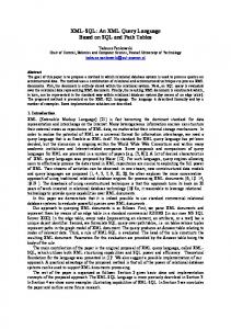
Fig. 2. Chain Dual Index: (a) queries; (b) dual index (lists not shown are empty; chd = child, dsc = desc); (c) a sample document; (d) CML lists; (e) PL lists: for brevity, only shown nodes 1 and 9; besides, only those entries of PL(9) not “inherited” from anestors of 9 are shown; (f) QL lists.

For chain labeling, the basic questions that need to be answered quickly are: (i) given a constant t, which queries contain an occurrence of t as a root?5 (ii) given a pair of constants ti ; t j , in which queries do they appear as a parent-child pair, and in which queries as an ancestor-descendant pair? 6 Notice that an ancestor-descendant pair (ti ; t j ) in a query Q means that t j is an ad-child of ti in Q. We call an access structure that supports efficient lookups of this form chain dual index. In our chain labeling algorithm, we denote lookup operations as DualIndex[t ℄(root ), DualIndex[ti ℄[t j ℄(child ), or DualIndex[ti ℄[t j ℄(desc), which respectively return the list of queries where t appears as the root tag, (ti ; t j ) appears as the tags/constants of a parent-child pair, and of an ancestor-descendant pair. E.g., Figure 2 (a)-(b) shows a sample chain dual index: e.g., DualIndex[a℄(root ) = fQ1; Q3; Q4g, DualIndex[a℄[b℄(child ) = fQ1g, and DualIndex[a℄[b℄(desc) = fQ4g. For tree labeling, the questions that need to be answered quickly are: (i) given a constant, which are the queries in which it occurs as a leaf and the node numbers of the occurrences, and what are the node numbers of the distinguished node of these queries, and (ii) given a tag, for each query in which it has a non-leaf occurrence, what 5 6

So, t must be a tag. Here, ti must be a tag, while t j may be a tag or a domain value.

are the node numbers of its pc-children and the node numbers of its ad-children? We call an access structure that supports efficient lookups of this form tree dual index. Figure 3(a)-(b) shows some queries and their associated tree dual index. In our tree labeling algorithm, we denote the above lookups as DualIndex[t ℄(L) and DualIndex[t ℄(N ) respectively. Each entry in DualIndex[t ℄(L) is of the form (P; l ; S), where P is a query, l is the number of its distinguished node, and S is the set of numbers of leaves of P with constant t. Each entry in DualIndex[t ℄(N ) is of the form (P; i; B; S; S0 ), where P is a query, i is the number a node in P with constant t, and S; S0 are respectively the sets of numbers of i’s pc-children and ad-children; finally, B is a boolean which says whether node i has an ad-parent in P (True) or not (False). The motivation for this additional bit will be clear in Section 5. Figure 3(b) illustrates the tree dual index for the sample set of queries in Figure 3(a). E.g., DualIndex[a℄(N ) contains the entries (P; 1; F; f2; 3g; fg) and (P; 4; T ; f6g; f5g). This is because a occurs at nodes 1 and 4 in query P. Of these, the first occurrence has nodes 2 ; 3 as its pc-children and no ad-children, while the second has pc-child 6 and ad-child 5. a (2)

b

b

(1)

(3) (4)

*c a

b

(2) (3)

(6) (4)

a *a (6)

c c

b

a

c

(5)

(1)

b (5)

P

c

N L N L N L

(P, 1, F, {2,3}. {}) (P, 3, {})

(Q, 1, F, {6}, {2}) (P, 3, {2,5}) (P,3,F,{},{4}) (P, 3, {6})

Q

(P, 4. T, {6}, {5})

(Q, 6, {4,6})

(Q, 6, {5}) (Q,2,T,{3},{})

(a)

c c a 5

2 9

3 8 4 d 6

b

7

(b)

a

1

b

a a

(Q, 3, F,{4}, {5})

(Q, 6, {})

c 10

d

11

c d 12 13 b

b 15

14

(c)

1 : (Q,2,6,?):desc. 2 : (Q,4,6,?):child, (Q,6,6,5):child, (P,6,3,?):child, (Q,2,6,?):child. 9 : (P,4,3,?):desc. 10: (Q,4,6,?):child, (Q,6,6,5):child, (P,4,3,?):child, (P,2,3,?):child, (P,5,3,?):child, (Q,5,6,?):child. 3 : (P,6,3,?):child, (Q,3,6,?):child. 11: (P,6,3,?):child, (P,2,3,?):desc, (P,5,3,?):desc, (Q,5,6,?):desc. 4 : (Q,4,6,?):child, (Q,6,6,5):child, (P,2,3,?):desc, (P,5,3,?):desc, (Q,5,6,?):desc. 13: (P,2,3,?):child, (P,5,3,?):child, (Q,5,6,?):child.

7 : (P,2,3,?), (P,5,3,?), (Q,5,6,?). 14: (P,2,3,?), (P,5,3,?), (Q,5,6,?). 5 : (Q,4,6,?), (Q,6,6,5). 12: (P,6,3,?). 6 : _. 13: _. 15: (P,2,3,?), (P,5,3,?), (Q,5,6,?). 4 : (P,6,3,?), (Q,3,6,?). 11: (Q,4,6,?), (Q,6,6,5), (P,4,3,?). 8 : (Q,4,6,?), (Q,6,6,5). 3 : (P,6,3,?), (Q,2,6,?). 10: _. 2 : (Q,1,6,5), (P,2,3,?), (P,5,3,?), (Q,5,6,?). 9 : (P,6,3,?), (P,3,3,9). 1 : (Q,4,6,?), (Q,6,6,5), (P,1,3,9). (d)

5: {Q} 9: {P} (f)

6 : (P,2,3,?):child, (P,5,3,?):child, (Q,5,6,?):child. (e)

Fig. 3. Tree Dual Index: (a) queries; (b) dual index; (c) sample document; (d)TML; (e)PL; (f) QL.

4 Chain Queries

In this section, we present an algorithm called Algorithm Node-Centric-Chain for chain labeling. Given a data tree, we seek to label each of its nodes with the list of chain queries that are answered by it. The main challenge is to do this with a small number of passes over the data tree, regardless of the number of queries, processing many queries at once. Figure 4 gives an algorithm for chain labeling. For expository reasons, in our presentation of query labeling algorithms in this and the next section, we associate several lists with each data tree node. We stress that in our implementation we compress these lists into a single one for reasons of efficiency [14].

With each data tree node, we associate three lists: the QL (for query labeling) list, which will eventually contain those queries answered by the (subtree rooted at the) node, a list called CML (for chain matching list) that tracks which queries have so far been matched and how far, and an auxiliary list called PL (for push list) that is necessary to manage CML. Each entry in the CML of a node u will be of the form (P; i; j; x), where P is a query, and i; j are non-negative integers, and x is either ‘?’ or is an integer. Such an entry signifies that there is a partial matching of the part of the chain P from its root down to the node whose distance from leaf is i, and j is the distance between the distinguished node and the leaf. In addition, when x is an integer, it says the data tree node with number x is the answer node corresponding to this matching. E.g., in Figure 2(d), for node 1 of the document, one of the CML entries is (Q1; 2; 0; ?), signifying that in query Q1, the part that includes only the query root (tag a) can be partially matched into node 1. The number 2 says the matched query node is at a distance7 2 from the query leaf, and the number 0 says the distinguished node is at distance 0 from the query leaf, i.e. it is the leaf. The ‘?’ says the location of the answer node for this matching is unknown at this point. Note that the CML associated with a data tree node may have multiple entries corresponding to the same query, signifying multiple matchings. Entries in PL are of the form (P; l ; m; x) : t, where P; l ; m; x are as above and t is a constant (tag). Such an entry belongs to the PL of a node u exactly when some ancestor of u in the document has tag t and the part of P from root down to the node with distance l to the leaf has been matched to this ancestor, and x has the same interpretation as above, i.e. the ancestor’s CML contains (P; l ; m; x). An entry (P; l ; m; x) can get into the CML of a data tree node u in one of two ways: (1) The root of P has tag identical to tag(u). In this case, l must be the height of P and m the distance from leaf to distinguished node. If l = m, we know the location of the answer node, viz., node u. (2) The CML of u’s parent in the document, say v, contains the entry (P; l + 1; m; x) and (tag(v); tag(u)) appears either as a pc-edge or as an ad-edge in query P. Note that the latter check can be performed by looking up the chain dual index via DualIndex[tag(v)℄[tag(u)℄(rel), where rel is either child or desc. It is possible that an ancestor (which is not the parent) v of u contains the entry (P; l + 1; m; x) instead. This should cause (P; l ; m; x) to be added to the CML of u, where x should be set to the number of node u if l = m, and left as ‘?’ otherwise. Instead of searching ancestors of u (which will make the number of passes large), we look for an entry of the form (P; l + 1; m; x) : t in the PL of u, such that (t ; tag(u)) appears as an ad-edge in query P. Here, t denotes the ancestor’s tag. This keeps the number of passes constant. Next, the PL is maintained as follows. Whenever an entry (P; l ; m; x) is added to the CML of a node u, the entry (P; l ; m; x) : tag(u) is added to the PL of u. Whenever x is set to a node number in a CML entry, the component x in the corresponding PL entry is also replaced. The contents of the PL of a node are propagated to its children. The following theorem shows there is an algorithm for chain labeling that makes two passes over the data tree. It assumes the existence of a chain dual index. Construction of dual indexes is discussed in [14]. As an example, in Figure 2(c), the CML of node 1 will initially get the entries (Q1; 2; 0; ?); (Q3; 2; 2; 1); (Q4; 2; 1; ?). In the second entry, the last component 1 says 7

Solid and dotted edges are counted alike for this purpose.

Algorithm Node-Centric-Chain Input: User queries Q1 ; :::; Qn ; Node labeled data tree T ; For simplicity, we use u also as the preorder rank associated with node u; Output: A query labeling of T ; 1. Initialize the lists CML, PL, and QL of every node to empty lists; 2. Traverse nodes of T in preorder; for each node u f 2.1. for every (Q 2 DualIndex[tag(u)℄(root )) f add (Q; h; d ; ?) to CML(u), where h is the height of Q and d is the distance of distinguished node from leaf; add (Q; h; d ; ?) : tag(u) to PL(u); if (h = d ) replace ‘?’ by u; //u is then a node to which the distinguished node of Q is matched. g 2.2. if (u has parent) f let v be the parent; 2.2.1. for every (Q 2 DualIndex[tag(v)℄[tag(u)℄(desc) [ DualIndex[tag(v)℄[tag(u)℄(child )) f if (9i; j; x : (Q; i + 1; j; x) 2 CML(v)) f add (Q; i; j; x) to CML(u) and tag(u) : (Q; i; j; x) to PL(u); if (x = ‘?0 ) f if (i = j) replace x by u; g g g 2.2.2. for every ((Q; i + 1; j; x) : t 2 PL(v)) f if (Q 2 DualIndex[t ℄[tag(u)℄(desc)) f add (Q; i; j; x) to CML(u) and tag(u) : (Q; i; j; x) to PL(u); if (x = ‘?0 ) f if (i = j) replace x by u; g g g 2.2.3. for every ((P; m; n; x) : t 2 PL(v)) add (P; m; n; x) : t to PL(u); g g 3. Traverse T postorder; for each node u f 3.1. for (every (P; 0; j; x) 2 CML(u)) f add P to QL(x); g g Fig. 4. Labeling Chain Queries: The Node-Centric Way

node 1 in the document is the answer node (corresponding to that matching). Figure 2(d)-(e) shows the CML and PL lists computed at the end of step 2 of the algorithm. Figure 2(f) shows the QL lists computed at the end of step 3. Note that the entry (Q4; 1; 1; 8) appears twice in CML(8). They are inserted by two different matchings, one that involves node 1 and another that involves node 5. In the figure, entries underlined by a dotted line indicate the first time (in step 2) when the component is replaced from a ‘?’ to a node number for those entries. Entries underlined by a solid line indicate successful completion of matchings (as indicated by the third component being zero). Theorem 1. (Chain Labeling) : Let T be a data tree and Q1 ; :::; Qn any set of chain queries. There is an algorithm that correctly obtains the query labeling of every node of T . The algorithm makes no more than two passes over T . Furthermore, the number of I/O invocations of the algorithm is no more than n  (2 + p), where n is the number

of nodes in the document tree and p is the average size of the node PL lists associated with data tree nodes.

5 Tree Queries In this section, we first discuss a direct bottom-up algorithm called Algorithm NodeCentric-Trees for tree labeling. As will be shown later, this algorithm makes just two passes over the data tree T and correctly obtains its query labeling w.r.t. a given set of queries which are general trees. 5.1 A Direct Algorithm Figure 5 shows Algorithm Algorithm Node-Centric-Trees. As with the chain labeling algorithm, we associate several lists with each node u in T . (1) The Tree Matching List (TML) contains entries of the form (P; l ; m; x) where P is a query, l the number of a node in P, m the number of the distinguished node of P, and x is either ‘?’ or the number of the node in T to which the distinguished node of P has been matched. (2) The push list (PL) contains entries of the form (P; l ; m; x) : rel where P; l ; m; x are as above and rel is either child or desc. It says there is a child or descendant (depending on rel) of the current node u whose TML contains the entry (P; l ; m; x). (3) The query labeling list (QL) contains the list of queries for which u is an answer node. These lists are managed as follows. Leaf entries in the tree dual index cause entries to be inserted into the TML lists of nodes. More precisely, let the current node u have tag t, and let DualIndex[t ℄(L) contain the entry (P; m; S). In this case, for every node l 2 S, we insert the entry (P; l ; m; ?) into T ML(u); in case l = m, we replace ‘?’ by the node number u. This signifies that the distinguished node of P has been matched into node u of T . Inductively, let (P; l ; B; C; D) be an entry in DualIndex[tag(u)℄(N ). If according to PL(u), for every c 2 C, there is a child of u into which the subtree of P rooted at c can be successfully matched, and for every d 2 D, there is a descendant of u into which the subtree of P rooted at d can be matched, then we add the entry (P; l ; m; x) to T ML(u). Here, the value of m is obtained from the entries in PL(u) that were used to make this decision. If at least one of the relevant PL(u) entries contains a value for x other than ‘?’, we use that value in the newly added entry in T ML(u); otherwise, we set x to ‘?’ in T ML(u). The PL list is first fed by entries added to T ML: for every entry (P; l ; m; x) added to T ML(u), we add the entry (P; l ; m; x) : child to PL( parent (u)). Secondly, whenever PL(u) contains the entry (P; l ; m; x) : rel, we add the entry (P; l ; m; x) : desc to PL( parent (u)). This latter step can result in an explosion in the size of the PL lists as every entry added to the PL of a node contributes entries to all its ancestors’ PL lists. This can be pruned as follows. Suppose PL(u) contains (P; l ; m; x) and suppose node l of query P has no ad-parent, i.e. either it has no parent or it has a pc-parent. In the former case, there is no need to “propagate” the PL entry from u to its parent. In the latter case, since the propagated entry would be (P; l ; m; x) : desc, it cannot contribute to the addition of any entry to PL( parent (u)). As an example, in Figure 3(c), there is a sample document. The figure illustrates how its query labeling is constructed by Algorithm Node-Centric-Trees w.r.t. the queries of Figure 3(a), including the details of the TML, PL, and QL lists. For instance, (P; 2; 3; ?) is added to T ML(7) since tag(7) = b and (P; 3; f2; 5g) belongs to DualIndex[b℄(L). As

Algorithm Node-Centric-Trees Input: User queries Q1 ; :::; Qn ; Node labeled data tree T ; Output: A query labeling of T ; 1. let h = height of T ; 2. for (i = h; i  0; i )f 2.1 for (each node u at level i) f 2.1.1. for (each (P; m; S) in DualIndex[tag(u)℄(L)) f for (each l in S) f add (P; l ; m; ?) to T ML(u); //base case entries if (l = m) replace ‘?’ by u; g g 2.1.2. for (each entry e in DualIndex[tag(u)℄(N )) f 2.1.2.1. let e be (P; l ; B; C; D); 2.1.2.2. if (not B) mask(P; l ) = true; //if u has no ad-parent, mask propagation of PL entries. 2.1.2.3. let R = f(m; x) j [8ci 2 C : (P; ci; m; y) : child 2 PL(u)& ((y = x) _ (y = ‘?0 ))℄ & [8di 2 D : ((P; ci; m; y) : child 2 PL(u)_ (P; ci; m; y) : desc 2 PL(u))&((y = x) _ (y = ‘?0 ))℄g; 2.1.2.4. if (R 6= 0/ ) f for (each (m; x) in R) f add (P; l ; m; x) to T ML(u); if (l = m) replace x by u; g g g 2.1.3 for (each entry (P; l ; m; x) in T ML(u)) f 2.1.3.1. add (P; l ; m; x) : child to PL( parent (u)); //Push that entry to the parent’s pushlist //indicating that this corresp. to a child edge. g 2.1.4. for (each entry (P; l ; m; x) : rel in PL(u)) f if (not mask(P; l )) add (P; l ; m; x) : desc to PL( parent (u)); g g 3. Traverse T preorder; for each node u of T f if ((P; l ; l ; x) is in T ML(u)) add P to QL(u); g Fig. 5. Labeling Tree Queries: The Node-Centric Way

an example of the inductive case for adding entries into TML, consider the addition of (Q; 3; 6; ?) into T ML(4). This is justified by the presence of (Q; 4; 6; ?) : child and (Q; 5; 6; ?) : desc in PL(4). The PL entries can be similarly explained. In the figure, those TML entries where the last component x gets defined for the first time are underlined in dotted line, whereas those entries which signify a complete matching (as indicated by l = 1) are underlined in solid line. Theorem 2. (Tree Labeling) : Let T be a data tree and Q1 ; :::; Qn any set of query trees. There is an algorithm that correctly obtains the query labeling of every node of T . The algorithm makes no more than two passes over T . Furthermore, the number of I/O invocations of the algorithm is at most 2  n, where n is the number of nodes of the document tree.

5.2 The Chain-Split Algorithm In this section, we develop an approach for tree labeling that builds on the previously developed approach for chain labeling. The main motivation of this approach is based on the assumption that matching chains is easier than matching arbitrary trees, so if a query contains many chains, it makes sense to exploit them. A chain in a query tree P is any path (x1 ; :::; xk ) such that every node xi ; 1 < i < k, has outdegree 1 in P.8 Such a chain is maximal provided: (i) either xk is a leaf of P, or it has outdegree > 1 and (ii) either x1 is the root of P, or it has outdegree > 1. In the sequel, by chains we mean maximal chains. For example, consider Figure 6(a). It shows four chains in query P – P1 = (1; 2); P2 = (1; 3; 4); P3 = (4; 5); P4 = (4; 6); similarly, there are four chains in query Q – Q1; Q2; Q3; Q4. Suppose we split given queries into chains and match them into the data tree. Then, we should be able to make use of the information collected about the various matchings of chains in matching the original queries themselves efficiently. For brevity, we only outline the main steps of the Chain-Split algorithm for tree labeling (instead of a formal description). We will need the following notions. A node of a query tree P is a junction node if it is either the root, or a leaf, or has outdegree > 1. In the chain split algorithm, we first match all the chains obtained from query trees using a chain dual index. In addition, we use an auxiliary data structure called junction index. The junction index is indexed by constants, just like the dual index. The index for any tag consists of entries of the form (P; n) : (Pi; li ); :::; (P j; l j ), where P is a query, Pi; :::; P j are its chains, and n; li ; :::; l j are node numbers in P. It says if a node u in a data tree satisfies the following conditions: (i) the chains Pi; :::; P j are matched into the data tree and u is the match of all their roots; (ii) vi ; :::; v j are the corresponding matches of their leaves9 ; (iii) the subtree of P rooted at li (resp., :::; l j ) is matched into the subtree of the data tree rooted at vi (resp., :::; v j ); then one can conclude that the subtree of P rooted at n is matched into the subtree rooted at u. In this sense, a junction index entry is like a rule with a consequent (P; n) and an antecedent(Pi; li); :::; (P j; l j ). Entries may have an empty antecedent. Note that the junction index may contain more than one entry for a given tag and a given query. Figure 6 illustrates how this algorithm works. A detailed exposition is suppressed for lack of space and can be found in [14]. A formal presentation of the chain split algorithm, omitted here for brevity, can be easily formulated from this exposition. A theorem similar to Theorem 2 can be proved for this algorithm as well.

6 Experiments We conducted a series of experiments to evaluate the effectiveness of the labeling algorithms developed. The algorithms presented were rigorously tested under different workloads. Experimental setup: Our MatchMaker system is implemented using JDK1.3, GnuC++2.96, and BerkeleyDB3.17 [2]. The requirements indexes, that we proposed are all disk resident and all other data structures are memory resident. The experiments were conducted 8 9

Note that all paths in our trees are downward. They need not be P’s leaves.

a

1

a

(P,4): (P3,5), (P4,6).

b

(P,2):

(P,5):

(P,1): (P1,2), (P2,4).

(Q,1): (Q1,3), (Q2,6).

(Q,4):

(Q,6):

(Q,3): (Q3,4), (Q4,5).

(P,6):

(2)

b

(1)

(3)

P3 (4) (5)

Q1

(1) Q2

(2)

c a (6) * c Q4 a b

c* a

(3)

c

(6)

(4)

P

3 Q

b

b P2 P4

a

(5)

Q (a)

1: (P1,1,_,_,1), (P2,2,1,_,1), (P3,1,_,_,1), (P4,1,_,_,1). 2: (P1,0,_,_,1), (Q1,2,_,_,2), (Q2,1,0,_,2). 3: (Q1,1,_,_,2), (Q3,1,_,_,3), (Q4,1,_,_,3). 4: (Q1,0,_,_,2), (Q1,1,_,_,2), (Q3,1,_,_,4), (Q4,1,_,_,4). 5: (Q3,0,_,_,4), (P1,1,_,_,5), (P2,2,1,_,5), (P4,1,_,_,5), (P3,1,_,_,5). 6: 7: (P3,0,_,_,1), (Q4,0,_,_,3), (Q4,0,_,_,4), 8: (P1,1,_,_,8), (P2,2,1,_,8), (P3,1,_,_,8), (P4,1,_,_,8), (Q2,0,0,8,2). 9: (P2,1,1,9,1), (Q3,1,_,_,9), (Q4,1,_,_,9). 10: 11: (P1,1,_,_,11), (P2,2,1,_,11), (P3,1,_,_,11), (P4,1,_,_,11), (P2,0,1,9,1). 12: (Q3,1,_,_,12), (Q4,1,_,_,12), (P2,1,1,12,11), (P4,0,_,_,11). 13: 14: (P3,0,_,_,11), (P3,0,_,_,1), (Q4,0,_,_,9). 15: (P3,0,_,_,1), (Q4,0,_,_,9).

(g)

3

8

a a

4

b

6

7

c 10

d b

11

c d 12 13 b

15

14

(b)

5: (Q,4,_,_), (Q,6,6,5). 7: (P,2,_,_), (P,5,_,_), (Q,5,_,_). 12: (P,6,_,_). 14: (P,2,_,_), (P,5,_,_).

15: (P,2,_,_), (P,5,_,_). 6: 13: 4: (Q,3,_,_), (P,6,_,_). 11: (Q,4,_,_), (Q,6,_,_), (P,4,_,_), 8: (Q,4,_,_), (Q,6,6,8). 3: (P,6,_,_). 10:

2: (P,2,_,_), (P,5,_,_), (Q,5,_,_), (Q,1,6,8).

(d)

1: {P}, 2:{Q}.

9

d 5

(c)

P1

2

c c

(Q,5):

a c

b

5: Q3: (Q,4,_,_,4), Q3:(Q,6,6,5,4). 7: P3:(P,2,_,_,1), P3:(P,5,_,_,1), Q4:(Q,5,_,_,3), Q4:(Q,5,_,_,4). 12: P4:(P,6,_,_,11). 14: P3:(P,2,_,_,11), P3:(P,2,_,_,1), P3:(P,5,_, _,11), P3:(P,5,_,_,1). 15: P3:(P,2,_,_,11), P3:(P,2,_,_,1), P3:(P,5,_,_,11), P3:(P,5,_,_,1). 6: inherit from 7. 13: inherit from 14. 4: inherit from 5 and 6; plus Q1:(Q,3,_,_,2). 11: inherit plus 12 and 13; plus P1:(P,4,_,_,11), P2:(P,4,_,_,11), P2:(P,4,_,_,1), P3:(P,4,_,_,11), P4:(P,4,_,_,11). 8: Q2:(Q,4,_,_,2), Q2:(Q,6,6,8,2). 3: P3:(P,2,_,_,1), P3:(P,5,_,_,1), Q4:(Q,5,_,_,3), Q1:(Q,3,_,_,2). 10: P2:(P,4,_,_,1), P3:(P,2,_,_,1), P3:(P,5,_,_,1), 2: P3:(P,2,_,_,1), P3:(P,5,_,_,1), Q1:(Q,3,_,_,2).Q2:(Q,4,_,_,2), Q2:(Q,6,6,8,2), P1:(P,2,_,_,1), P1:(P,5,_,_,1), Q1:(Q,5,_,_,2), Q1:(Q,1,6,8,2), Q2:(Q,5,_,_,2), Q2:(Q,1,6,8,2).

9: (P,6,_._).

9: P2:(P,4,4,9,1), P3:(P,2,_,_,1),

1: (Q,4,_,_), (Q,6,6,1), (P,1,3,9).

1: inherit from 2 and 9, entries with last component