On-line Bushing Condition Monitoring

Proc. of the 5th WSEAS/IASME Int. Conf. on Electric Power Systems, High Voltages, Electric Machines, Tenerife, Spain, December 16-18, 2005 (pp406-411)

On-line Bushing Condition Monitoring C.B. VILAKAZI, R.P. MAUTLA, E.M. MOLOTO and T. MARWALA School of Electrical and Information Engineering University of the Witwatersrand Private Bag 3, Wits, 2050 SOUTH AFRICA

Abstract: – An on-line bushing condition monitoring framework is presented, the framework is able to adapt as new data are introduced. Furthermore, it can accommodate new classes that are introduced by incoming data. The framework is implemented using an incremental learning algorithm that uses MLP as a weak Learner. The performance of the on-line bushing condition monitoring is compared to that of an MLP trained off-line. The proposed framework is able to adapt as new data are introduced and is able to accommodate new classes. The testing results improved from 67.5% to 95.8% as new data are introduced and the testing results improved from 60% to 95.3% as new classes are introduced. On average the confidence value of the framework on its decisions is 0.92. Key-Words: – Bushing, dissolve gas-in-oil analysis (DGA), multi-layer perceptrons (MLP), incremental learning, Learn++, weak Learn, hypothesis

1

Introduction

Bushings are critical components in transmission and distribution of electricity. The reliability of the bushings not only affects the electric availability of the supplied area but also the economical operation of a utility. Various diagnostics tools have been used to detect bushings and transformer failures. These include techniques such as on-line partial discharge (PD) analysis, on-line power factor, infrared scanning, temperature monitoring, vibration monitoring and chemical techniques [1]. However, few of these methods can in isolation provide all of the information that a transformer operator requires to diagnose failures. Among chemical techniques, dissolve gas analysis (DGA) has gained worldwide recognition as a diagnostic method for detecting incipient faults [3][4]. Artificial neural networks (ANN) have been used in the past for bushing and transformer condition monitoring [4][5][6][7] but the main shortcomings of the methods proposed to date is that they do not take into account the on-line implementation requirement. As a consequence of this shortcoming, the paper proposes a new method for interpreting bushing data from the DGA test using multi-layer perceptrons (MLP) with on-line learning capability. The basis of many artificial intelligence based methods for bushing diagnosis relies heavily on adequate and representative set of training. It is also often common that the training data becomes available only in small batches and that some new classes only appear in subsequent data collection

stage. Hence, there is a need to update the classifier in an incremental fashion without compromising on the classification performance of previous data. In this paper, an on-line learning that uses an incremental learning algorithm using MLP neural network is proposed for bushing condition monitoring.

2

Background

This section gives background on dissolve gas analysis, artificial neural networks and incremental learning algorithms.

2.1

Dissolve gas analysis

Dissolve gas analysis is the most commonly used diagnostic technique for transformers and bushings [3]. DGA is used to detect oil breakdown, moisture presence and PD activity. Fault gases are produced by degradation of transformer and bushing oil and solid insulation such as paper and pressboard, which are all made of cellulose [3][8]. The gases produced from the transformer and bushing operation are divided into three groups and these are: hydrocarbons gases group, which are methane (CH4), ethane (C2H6), ethylene (C2H4), acetylene (C2H2) and hydrogen (H2); the carbon oxide group, which includes carbon monoxide (CO) and carbon dioxide (CO2); and the non-fault gases, which are nitrogen (N2) and oxygen (O2). The nature of faults is classified into two main groups and these are discharges and thermal heating. Partial discharge faults are divided into high-energy

Proc. of the 5th WSEAS/IASME Int. Conf. on Electric Power Systems, High Voltages, Electric Machines, Tenerife, Spain, December 16-18, 2005 (pp406-411)

discharge and low energy discharge. The high-energy discharge is known as arcing and low energy discharge is referred to as corona. The quantity and types of gases reflect the nature and extent of the stressed mechanism in the bushing [3]. Oil breakdown is shown by the presence of hydrogen, methane, ethane, ethylene and acetylene. High levels of hydrogen show that the degeneration is due to corona. High levels of acetylene occur in the presence of arcing at high temperature. Methane and ethane are produced from low temperature thermal heating of oil and high temperature thermal heating produces ethylene, hydrogen as well as a methane and ethane. Low temperature thermal degradation of cellulose produces CO2 and high temperature produces CO.

2.2 Artificial neural networks Artificial neural networks are data processing system that learns complex input-output relationships from data. A typical ANN consists of simple processing elements called neurons that are highly interconnected in an architecture that is loosely based on the structure of biological neurons in human brain. There are different types of ANN models; two that are commonly used are MLP network and radial basis function (RBF) network. However, only MLP are implemented in this paper because they have been successfully applied to various condition monitoring applications [4][5]. Fig. 1 shows the architecture of an MLP with four neurons in the input layer, three neurons in the hidden layer and two neurons in the output layer.

Fig. 1. Architecture of an MLP Fig.1 shows the relationship between input (x) and output (y), which can be written as [9]    N 2  d 1 yj = f ∑ w f ∑ w x   j = 0 kj  i = 0 ji i     

(1)

In (1), w ( 2) and w (1) represents the weight of the kj

ji

layer 2 and layer 1, respectively, N is the number of ouput units and d is the number of hidden units. 2.3 Incremental learning An incremental learning algorithm is defined as an algorithm that learns new information from unseen data, without necessitating access to previously used data [10]. The algorithm must also be able to learn new information from new data and still retains knowledge from the original data. Lastly, the algorithm must be able to learn new classes that may be introduced by new data. This type of learning algorithm is sometimes referred to as a ‘memoryless’ on-line learning algorithm. Learning new information without requiring access to previously used data, however, raises ‘stability-plasticity dilemma’ [11]. This dilemma indicates that a completely stable classifier maintains the knowledge from previously seen data, but fails to adjust in order to learn new information, while a completely plastic classifier is capable of learning new data but lose prior knowledge [12]. The problem with MLP is that it is a stable classifier and is not able to learn new information after it has been trained Different procedures have been implemented for incremental learning. One procedure of learning new information from additional data involves discarding the existing classifier and training a new classifier using accumulated data [13][14]. Other methods such as pruning of networks or controlled modification of classifier weight or growing of classifier architectures are referred to as incremental learning algorithm. This involves modifying the weights of the classifier using the misclassified instances only. The above algorithms are capable of learning new information, however, they suffer from ‘catastrophic forgetting’ and require access to old data [15][16]. One approach evaluates the current performance of the classifier architecture. If the present architecture does not sufficiently represent the decision boundaries being learned, new decision clusters are generated in response to new pattern. Furthermore, this approach does not require access to old data and can accommodate new classes. However, the main shortcomings of this approach are: cluster proliferation and extreme sensitivity to selection of algorithm parameters [17]. In this paper, Learn++ is implemented for on-line learning of bushing

Proc. of the 5th WSEAS/IASME Int. Conf. on Electric Power Systems, High Voltages, Electric Machines, Tenerife, Spain, December 16-18, 2005 (pp406-411)

condition monitoring. The Learn++ algorithm is summarized in the next section.

3

Learn++

Learn++ is an incremental learning algorithm that uses an ensemble of classifiers that are combined using weighted majority voting [11]. Learn++ was developed by Polikar [11] and was inspired by a boosting algorithm called adaptive boosting (AdaBoost). Each classifier is trained using a training subset that is drawn according to a distribution. The classifiers are trained using a weak Learn algorithm. The requirement for the weak Learn algorithm is that it must be able to give a classification rate of less than 50% initially [12]. For each database Dk that contains training sequence, S, where S contains learning examples and their corresponding classes, Learn++ starts by initializing the weights, w, according to the distribution DT, where T is the number of hypothesis. Initially the weights are initialized to be uniform, which gives equal probability for all instances to be selected to the first training subset and the distribution is given by

D= 1

(2)

m

where m represents the number of training examples in Sk. The training data are then divided into training subset TR and testing subset TE to ensure weak Learn capability. The distribution is then used to select the training subset TR and testing subset TE from Sk. After the training and testing subset have been selected, the weak Learn algorithm is implemented. The weak Learner is trained using subset, TR. A hypothesis, ht, obtained from weak Learner is tested using both the training and testing subsets to obtain an error, εt: Dt (i ) εt = (3)

∑

t :hi ( xi ) ≠ yi

The error is required to be less than 0.5; a normalized error βt is computed using:

βt = ε t 1 − ε

(4) t

If the error is greater than 0.5, the hypothesis is discarded and new training and testing subsets are selected according to DT and another hypothesis is computed. All classifiers generated so far, are combined using weighted majority voting to obtain composite hypothesis, Ht (5) H t = arg max log(1 / β t ) y∈Y

∑

t :hi ( x ) = y

Weighted majority voting gives higher voting weights to a hypothesis that performs well on the training and testing subsets. The error of the composite hypothesis is computed as in (3) and is given by (6) Et = Dt (i )

∑

t : H i ( xi ) ≠ y i

If the error is greater than 0.5, the current hypothesis is discarded and the new training and testing data are selected according to the distribution DT. Otherwise, if the error is less than 0.5, the normalized error of the composite hypothesis is computed as:

Bt =

Et

(7)

1 − Et

The error is used in the distribution update rule, where the weights of the correctly classified instances are reduced, consequently increasing the weights of the misclassified instances. This ensures that instances that were misclassified by the current hypothesis have a higher probability of being selected for the subsequent training set. The distribution update rule is given by

wt +1 = wt (i ) × Bt

1−[| H t ( xi ) ≠ yi |]

(8) Once the T hypothesis is created for each database, the final hypothesis is computed by combining the hypothesis using weighted majority voting given by K

H t = arg max ∑ y∈Y

3.1

∑ log(1 / β ) t

(9)

k =1 t:H t ( x ) = y

Confidence measurement

A simple procedure is used to determine the confidence of the algorithm on its own decision. A vast majority of hypothesis agreeing on a given instances can be interpreted as an algorithm having confidence in its own decision. Let us assume that a total of T hypothesis are generated in k training session for a C-class problem. For any given example, the final classification is class, if the total vote class c receives ξc = ψt , (10)

∑

t:ht ( x ) = c

where ψt denotes the voting weights of the tth, hypothesis ht. Normalizing the votes received by each class gives

γ c= ξ c

C

∑ξc

(11)

c =1

γc can be interpreted as a measure of confidence on a scale of 0 to 1. A high value of γc show high

Proc. of the 5th WSEAS/IASME Int. Conf. on Electric Power Systems, High Voltages, Electric Machines, Tenerife, Spain, December 16-18, 2005 (pp406-411)

confidence in the decision and consequently, a low value of γc show low confidence in the decision. It should be noted that the γc value does not represent the accuracy of the results but the confidence of the system on its own decision. The classification rate is also used to measure the performance of the proposed framework and is defined simply as the rate of the incorrectly classified instances to the correctly classified instances.

4

Bushing condition framework

monitoring

The proposed method for fault diagnosis is a twostage implementation. The first stage of the diagnosis identifies if the bushing is faulty or not. If the bushing is faulty, the second phase determines the types of faults, which are thermal fault, PD faults and faults caused by unknown source. Generally, the procedure of fault diagnosis includes three steps, extracting feature and data pre-processing, training the classifiers and identifying transformer fault with the trained classifiers. Fig.2 shows the block diagram of the proposed methodology. Feature Extracting and Pre-processing

Classifier

Is bushing Faulty?

No

Normal Operation

Yes

Classifier

4.2

MLP classifier

When implementing the MLP, the choice of architecture is an important design decision as it determines the generalisation capability of the network. In selecting the architecture, issues such as model complexity and over-fitting have to be taken into consideration. An MLP with two layers is implemented in this paper as previous work on optimal number of hidden layer has shown that a sufficiently large network with one hidden layer of neurons is able to approximate any function with arbitrary accuracy [18]. The optimal number of hidden layer can be found by using exhaustive search. MLP is trained using the scaled conjugate gradient training method. Cross-validation is used to ensure that a network with good generalization property is achieved. In this paper MLP is trained using batch learning. Batch learning implies that all available data are used to train an MLP and that the network does not have incremental capability. Additionally, the MLP is used as a weak Learner in the Learn++ algorithm.

5

Experimental results

The first experiment evaluate the incremental capability of the algorithm is tested using first phase, which is to determine whether the bushing is faulty or not. The data used was collected from

What Type of fault?

Partial Discharge Unknown Fault Fault

standards [7]. Data pre-processing is an integral part of neural network architecture. Data pre-processing makes it easier for the network to learn. Data are normalized to fall within 0 and 1, using linear normalization.

Thermal Fault

Fig.2. Block diagram of the proposed methodology 4.1 Data Preprocessing DGA is used to determine the faulty gases in the bushing oil. The content information reflects the states of the transformer and bushing. Ten diagnostic gases mentioned in Section 2 are extracted, which are CH4, C2H6, C2H4, C2H2, H2, CO, CO2, N2, O2 and total dissolved combustible gases. The total dissolved combustible gas is given by the sum of methane, hydrogen, acetylene, ethane, ethylene and hydrogen. The faulty gases are analysed using the IEEE C57.104

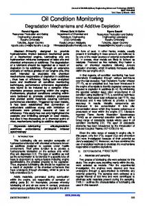
bushing over a period of 2.5 years of bushings in services. The algorithm is implemented with 1500 training examples and 4000 validation examples. The training data were divided into five databases each with 300 training instances. In each training session, Learn++ is provided with each database and generates 20 hypotheses. The weak Learner uses an MLP with 10 input layer neurons, 5 hidden layer neurons and one output layer neuron. To ensure that the method retains previously seen data, for each training session, the previous database is tested. The first row of Table 1 shows the performance of the Learn++ on the training data for different databases. On average weak Learner gives 60% classification rate on its training dataset, which improves to 98% when the hypotheses are combined.

Proc. of the 5th WSEAS/IASME Int. Conf. on Electric Power Systems, High Voltages, Electric Machines, Tenerife, Spain, December 16-18, 2005 (pp406-411)

This demonstrates the performance improvement of Learn++ as inherited from AdaBoost on a single database. Fig. 2 shows the performance of Learn++ on training dataset against the number of classifiers for a single database. Each column thereafter shows the performance of current and previous databases and this is to show that Learn++ does not forget previously learned information, when new data are introduced. The last row of Table 1 shows the classifiers performances on the testing dataset, which gradually improved from 65.7% to 95.8% as new databases become available thereby demonstrating incremental learning capability of Learn++. Fig. 4 shows the performance of Learn++ on one data set against the number of datasets. Table 2 shows that the confidence of framework increases as new data are introduced. Table 1: Performance of Learn++ for first stage online bushing condition monitoring. Key: S = data Dataset S1 S2 S3 S4 S5 S1 89.5 85.8 83.00 86.9 85.3 93.7 92.9 S2 ─ 91.4 94.2 90.1 91.4 S3 ─ ─ 93.2 S4 ─ ─ ─ 92.2 94.5 S5 ─ ─ ─ ─ 98.0 Testing (%) 65.7 79.0 85.0 93.5 95.8 94 92 90

) % ( y c a r u c c a n o ti a c fii s s a l c

88 86

The second experiment was performed to evaluate whether the MLP can accommodate new classes. The faulty data were divided into 1000 training examples and 2000 validation data, which contain all the three classes. The training data were divided into five databases, each with 200 training instances. The first and second databases contain training examples of PD and thermal faults. The data of unknown fault is introduced in the third training session. In each training session, Learn++ is provided with each database and generates 20 hypotheses. The last row of Table 3 shows that the classifiers performances increases from 60% to 95.3% as new classes are introduced in the subsequent training dataset. Table 3: Performance of Learn++ for second stage bushing condition-monitoring key: S = databases Dataset S1 S2 S3 S4 S5 95.7 95.1 S1 95.0 95.2 94.6 96.8 95.3 S2 ─ 96.3 96.0 96.4 96.5 S3 ─ ─ 97.0 S4 ─ ─ ─ 97.8 96.8 S5 ─ ─ ─ ─ 99.2 Testing (%) 60.0 65.2 76.0 83.0 95.3

84 82 80 78 76

0

2

6

4

12 10 8 number of classifiers

14

16

18

20

Fig.3. Performance of Learn++ on training dataset against the number of hypothesis

The last experiment addressed the problem of bushing condition monitoring using MLP network trained using batch learning. This was done to compare the classification rate of Learn++ with that of an MLP. An MLP with the same set of training example as Learn++ was trained and the trained MLP was tested with the same validation data as Learn++. This was done for the first stage, which is a two-class and second stage, which is a three-class problem. The first phase MLP gave classification rate of 97.2%, whereas the second phase MLP gave a classification rate of 96.0%.

100

95

) % ( y c a r u c c a n o ti a c fii s s a l c

Table 2: The confidence of the algorithm for classified cases for all databases and for each class. S1 S2 S3 S4 S5 Classified: Normal Class 0.66 0.85 0.92 0.94 0.94 0.49 0.64 0.81 0.90 0.90 Faulty Class

90

85

80

75

70

65

1

2

3 number of databases

4

5

Fig.4. Performance of Learn++ on testing data against the number of databases

6

Discussion and conclusions

Current bushing condition monitoring techniques provide promising results but lack the

Proc. of the 5th WSEAS/IASME Int. Conf. on Electric Power Systems, High Voltages, Electric Machines, Tenerife, Spain, December 16-18, 2005 (pp406-411)

incremental capability if they are to be used for automatic and continuous on-line monitoring. In this paper, a method for on-line learning that uses incremental learning is implemented for on-line bushing condition monitoring. The proposed online bushing condition monitoring framework consists of two stages. The first stage determines if the bushing is faulty or not and the second stage determines the nature of the fault. Experimental results demonstrate that the proposed framework has incremental learning capability. Furthermore, these results show that the framework is able to accommodate new classes introduced by incoming data. The results further show that the algorithm has a high confidence in its own decision and this confidence increases as additional data are introduced.

References: [1] B. Ward, “A survey of new techniques in insulation monitoring of power transformers”, IEEE Electrical Insulation Magazine, vol.17, no.3, 2000, pp.16-23. [2] T.K. Saha, “Review of modern diagnostic techniques for assessing insulation condition in aged transformer”, IEEE Transactions on Dielectric and Electrical Insulation, vol.10, no.5, 2003, pp. 903-917. [3] S.M Dhlamini, T. Marwala, “An application of SVM, RBF and MLP with ARD on bushings”, Proceedings of the IEEE Conference on Cybernetics and Intelligent System, pp. 12451258, 2004. [4] T. Marwala. Fault identification using neural networks and vibration data. Doctor of Philosophy Thesis, University of Cambridge, 2001. [5] X. Ding, Y. Liu, P.J Griffin, ”Neural nets and experts system diagnoses transformer faults”, IEEE Computer Applications in Power in Power, vol. 13, no. 1, 2000, pp. 50-55. [6] T. Yanming, Q. Zheng, “DGA based Insulation Diagnosis of Power Transformer via ANN”, Proceedings of the 6th International Conference on Properties and Application of Dielectric Materials, vol.1, 2000, pp. 133-137. [7] A.R.G. Castro, V. Miranda, ”An interpretation of neural networks as inferences engines with application to transformer failure diagnosis”,

International Journal of Electrical Power and Energy Systems, 2005 (in press). [8] “IEEE Guide for the interpretation of Gases generated in Oil-immersed Transformer”, IEEE Standard C57.104-1991, 1991, pp.1-30. [9] I.T Nabney, Netlab algorithms for pattern recognition, London, Springer, 2003. [10] S. Lange, G. Grieser, ”On the power of incremental learning,” Theory of Computer Science, vol. 288, no. 2, 2002, pp. 277-307. [11] R. Polikar, L. Udpa, S. Udpa, V. Honavar, “Learn++: An incremental learning algorithm for supervised neural networks,” IEEE Transactions on System, Man and Cybernetics (C), Special Issue on Knowledge Management, vol. 31, no. 4, 2001, pp. 497-508. [12] R. Polikar, L. Udpa, S. Udpa, , V. Honavar “An incremental learning algorithm with confidence estimation for automated identification of NDE signals,” IEEE Transactions on Ultrasonic Ferroelectrics, and Frequency control, vol. 51, no. 8, 2004, pp. 990-1001. [13] Higgins C.H, Goodman R.M, “Incremental learning for rule based neural network”, Proc. International. Joint Conference on Neural Networks, vol. 1, 1991, pp. 875-880. [14] M. McCloskey, N. Cohen, “Catastrophic interference connectionist networks: The sequential learning problem”, The Psychology of Learning and Motivation, vol. 24, 1989, pp. 109164. [15] L. Fu, H.H. Hsu, J.C Principe “Incremental backpropagation networks”, IEEE Trans. Neural Network, vol. 7, no. 3, 1996, pp. 757 -761. [16] K. Yamaguchi, N. Yamaguchi and N. Ishii, “Incremental learning method with retrieving of interfered patterns”, IEEE Transactions on. Neural Networks, vol. 10, no. 6, 1999, pp. 13511365 [17] G.A Carpenter, S. Grossberg, N. Marhuzon, J.H Reynolds and D.B Rosen, “ARTMAP: A neural network architecture for incremental learning supervised learning of analog multidimensional maps,” IEEE Trans. Neural Networks, vol 3, no. 5, 1992, pp. 698-713. [18] C.M. Bishop, Neural Network in Pattern Recognition, Oxford, Oxford University Press, 1995.