4300 Varsity Drive, Suite C,. Ann Arbor, MI 48108. On-Line Seam Detection in. Rolling Processes Using Snake. Projection and Discrete Wavelet. Transform.
Jing Li Jianjun Shi Department of Industrial and Operations Engineering, The University of Michigan, 1205 Beal Avenue, Ann Arbor, MI 48109-2117
Tzyy-Shuh Chang OG Technologies, Inc., 4300 Varsity Drive, Suite C, Ann Arbor, MI 48108
On-Line Seam Detection in Rolling Processes Using Snake Projection and Discrete Wavelet Transform This paper describes the development of an on-line quality inspection algorithm for detecting the surface defect “seam” generated in rolling processes. A feature-preserving “snake-projection” method is proposed for dimension reduction by converting the suspicious seam-containing images to one-dimensional sequences. Discrete wavelet transform is then performed on the sequences for feature extraction. Finally, a T2 control chart is established based on the extracted features to distinguish real seams from false positives. The snake-projection method has two parameters that impact the effectiveness of the algorithm. Thus, selection of the parameters is discussed. Implementation of the proposed algorithm shows that it satisfies the speed and accuracy requirements for on-line seam detection. 关DOI: 10.1115/1.2752519兴 Keywords: seam detection, discrete wavelet transform (DWT), feature extraction, T2 control chart
1
Introduction
Rolling is a high-speed bulk deformation process that reduces the thickness or changes the cross section of a long workpiece by compressive forces applied through a set of rolls 关1兴. Surface defects are critical quality concerns in the rolling industry. They are usually generated due to material overfills, nonmetallic inclusion, or porosities. Among surface defects, a seam is one of the most serious types. Because seams result in stress concentration on the bulk material that could cause catastrophic failures when the rolled product is in use, products with severe seams have to be scraped. Therefore, detection of seams is important for quality assurance. Seam detection has traditionally been restricted to off-line manual inspection because of a lack of effective sensors that can inspect the product surface on-line, under harsh environmental conditions, such as heat, dust, and lubricants. In recent years, with the development of advanced imaging technologies, vision sensors have been successfully adopted in the rolling process, collecting high-quality sensing images of the product surface. As a result, automatic on-line detection of seams becomes possible. A portion of a sensing image from a bar-rolling process 共i.e., the products are steel bars兲 is given in Fig. 1. Because a seam has a high contrast against its background in terms of image gray levels, as shown in Fig. 1, edge detection techniques can be adopted to detect seams. A qualified edge detector should possess two properties for on-line seam detection. First, considering the rolling velocity, 100% inspection of the product surface requires a data processing speed of at least 80 Mb/ s. Thus, the edge detector should be computationally fast. Second, the sensing images are noisy, as seams usually intermix with surface marks and material impurities. Therefore, for effectively identifying seams and reducing the false alarm rate, the edge detector should be noise insensitive. In the edge detection literature, although some edge detectors, such as Prewitt detectors and Sobel detectors 关2兴, are simple and fast, their performance Contributed by the Manufacturing Science Division of ASME for publication in the JOURNAL OF MANUFACTURING SCIENCE AND ENGINEERING. Manuscript received December 1, 2004; final manuscript received May 3, 2007. Review conducted by C. James Li.
926 / Vol. 129, OCTOBER 2007
deteriorates unacceptably when the image is noisy. More sophisticated edge detectors use smoothing operations to reduce noise 关2兴, but some useful information for detecting edges is inevitably lost. Optimal detectors 关3兴 were proposed to ensure an acceptable compromise between noise reduction and edge conservation. A typical optimal detector is called “Canny,” which has been extensively used as a standard gauge in the edge detection research 关4兴. However, optimality is achieved with a sacrifice in the detection speed. Other edge detection approaches include multiscale methods, statistical tools, and neural networks 关5兴, which are computationally more intensive. To detect seams fast and effectively under noisy rolling surface conditions, a two-stage seam detection methodology has been developed in this research. In the first stage, a Sobel edge detector is adopted to rapidly identify the suspicious seam-containing local regions 共referred to as sub-images from here on兲 in a sensing image. As the Sobel edge detector is noise sensitive, a large number of the identified sub-images are indeed false positives. Thus, a re-inspection on the sub-images is needed in the second stage to distinguish real seams from false positives. Because the subimages have a substantially smaller size than the original sensing images, a more sophisticated algorithm can be adopted. The developed re-inspection algorithm consists of three steps: 共i兲 converting the sub-images into 1-D sequences by a proposed snakeprojection method that reduces the data dimension while preserving seam characteristics; 共ii兲 extracting features from the sequences by discrete wavelet transform 共DWT兲; and 共iii兲 identifying seams by a T2 control chart based on the extracted features. Because the Sobel edge detector in the first-stage seam detection methodology is well documented in the literature, this paper focuses on the development of the second-stage algorithm 共referred to as snake-projection-wavelet algorithm兲. The remainder of this paper is organized as follows. Section 2 gives a brief description of the sub-images and data structure. Section 3 provides the detailed procedure for developing the snake-projectionwavelet algorithm. Section 4 presents a case study to demonstrate the effectiveness of the developed algorithm. Finally, Sec. 5 summarizes this research.
Copyright © 2007 by ASME
Transactions of the ASME
Downloaded 14 Jan 2008 to 129.219.244.213. Redistribution subject to ASME license or copyright; see http://www.asme.org/terms/Terms_Use.cfm
Fig. 1 A portion of a sensing image from a bar-rolling process
Fig. 3 „a… Two ridge-based false positive sub-images „left: containing two dark strips; right: containing one dark strip…, „b… a mark-based false positive sub-image
Fig. 2 A seam sub-image
2
Description of Sub-Images and Data Structure
This section introduces the physical forms of seams and false positives, their appearances in sub-images, and the structure of the sub-image data.
2.1 Seam and False Positive: Physics and Image Appearance. A seam is a thin deep crack along the longitudinal direction of a rolling bar. Thus, it shows as a nearly vertical thin dark strip with a constant width of 2 – 3 pixels in the sensing image. Figure 2 is a seam-containing sub-image. There are two types of false positives: ridge based and mark based, as shown in Fig. 3. A ridge-based false positive is a longitudinal ridge on the surface caused by material overfills. It is
冤
a11
¯
usually pictured as a thin bright strip with one or two dark strips on its sides, depending on the angle of the lighting source, where the bright and the dark strips are the ridge and its shadow共s兲, respectively. A mark-based false positive is a longitudinal mark on the surface, usually characterized by a dark strip of varying width. Note that, although the false positives have different physical forms and image patterns, they each have a dark strip in the subimages, which is misidentified as a seam. However, in the ridgebased false positive, the dark strip is paralleled by a bright strip 共i.e., the ridge兲; and in the mark-based false positive, the width of the dark strip 共i.e., the mark兲 varies. These two characteristics form the fundamental difference between false positives and seams. 2.2 Data Structure of Sub-Images. The data of a sub-image is a matrix with each element corresponding to one image pixel. The elements take integer values ranging from 0 to 255 gray levels, where 0 and 255 represent black and white, respectively. A typical matrix for one sub-image containing m ⫻ n pixels is given in 共1兲, where aij is the gray level of the pixel at the ith row and the jth column 共0 ⱕ aij ⱕ 255兲:
¯
a1共t1−k兲
¯
a1共t1−1兲
a= 1t1
a1共t1+1兲
¯
a1共t1+k兲
¯
¯
a1n
a= 2t2
a2共t2+1兲
a21
¯
¯
a2共t2−k兲
¯
a2共t2−1兲
¯
a2共t2+k兲
¯
¯
a2n
⯗
⯗
⯗
⯗
⯗
⯗
⯗
⯗
⯗
⯗
⯗
⯗
⯗
ai1
¯ ai共ti−k兲
¯
ai共ti−1兲
a= iti
ai共ti+1兲
¯
ai共ti+k兲
¯
¯
¯
ain
⯗
⯗
⯗
⯗
⯗
⯗
⯗
⯗
⯗
a共m−1兲1 ¯
¯
a共m−1兲共tm−1−k兲
¯
¯
¯
¯
am共tm−k兲
am1
a共m−1兲共tm−1−1兲 a= 共m−1兲tm−1 a共m−1兲共tm−1+1兲 ¯
Journal of Manufacturing Science and Engineering
am共tm−1兲
a= mtm
⯗
⯗
⯗
⯗
¯
a共m−1兲共tm−1+k兲
¯
¯ a共m−1兲n
am共tm+1兲
¯
am共tm+k兲 ¯
amn
冥
共1兲
OCTOBER 2007, Vol. 129 / 927
Downloaded 14 Jan 2008 to 129.219.244.213. Redistribution subject to ASME license or copyright; see http://www.asme.org/terms/Terms_Use.cfm
In addition to the matrix, the location of the center line of the dark strip in the sub-image is also taken as input to the snakeprojection-wavelet algorithm. This location is identified by the Sobel edge detector and recorded in a vector 关t1 , . . . , ti , . . . , tm兴T, where ti is the column index of element aiti 共i = 1 , 2 , . . . , m兲 on the center line of the dark strip. Because a dark strip is not strictly vertical, ti is not necessarily equal to t j 共1 ⱕ i , j ⱕ m , i ⫽ j兲. Thus, elements 关a1t1 , . . . , aiti , . . . , amtm兴T form a curved line along the vertical direction. This line, shown in 共1兲 by the elements with double underlines, is referred to as the “characteristic line” of a sub-image in this paper. Physically, the characteristic lines of a seam sub-image, a ridge-based false positive sub-image, and a mark-based false positive sub-image correspond to the center lines of the seam, one shadow strip of the ridge, and the mark, respectively. Detailed procedures for obtaining a sub-image matrix as well as the characteristic line can be found in 关6兴.
3
Snake-Projection-Wavelet Algorithm
The procedure of the snake-projection-wavelet algorithm is shown in Fig. 4. The sub-images are first converted to 1-D sequences by a feature-preserving snake-projection method. A discrete wavelet transform is then performed on the sequences for feature extraction. Finally, a T2 control chart is constructed, based on the features to distinguish seams from false positives. 3.1 Dimension Reduction by a Feature-Preserving SnakeProjection Method. Dimension reduction samples the pixels in the sub-image and converts the sub-image into a 1-D sequence. With fewer pixels and reduced dimension, the computational speed of the algorithm can be increased. In dimension reduction, it is important that the features that distinguish seams from false positives are preserved. These features are embedded in the row pixels of the sub-image. To further illustrate this point, three rows are extracted from each sub-image in Figs. 2 and 3, with the gray levels of the pixels on each row plotted on the right-hand side of the sub-image. 共The arrows on the left-hand side indicate the lo-
Fig. 4
Procedure of the snake-projection-wavelet algorithm
cations of the three rows.兲 It can be seen that 共i兲 a ridge-based false positive differs from a seam in the shape of the curves, and 共ii兲 the width of the valleys in the curves of a mark-based false positive varies while this width in the curves of a seam is almost constant. Therefore, to capture the shape difference and the width variation, multiple rows need to be extracted from a sub-image, which motivates the following “snake-projection” method. Step 1. Extract the elements 兵ai共ti−k兲 , ai共ti−k+1兲 , . . . , ai共ti−1兲 , aiti , ai共ti+1兲 , ai共ti+2兲 , . . . , ai共ti+k兲 : i = 1 , 2 , . . . , m其 from 共1兲, i.e., extract the pixels on the characteristic line, together with k adjacent pixels on each side of the line for each row of a sub-image. The extracted elements constitute a m ⫻ 共2k + 1兲 matrix, as shown in 共2兲. In this matrix, the characteristic line corresponds to the center column. Step 2. In 共2兲, extract the elements on every s row and the elements on the endmost columns connecting those rows. The inclusion of the endmost columns helps maintain the continuity of gray levels between two extracted rows. The extracted elements, highlighted by gray strips in 共2兲, constitute a sequence in which the ordering of the elements is specified by the arrows. This sequence is denoted by a vector Vk,s.
共2兲
Due to the shape of the connective gray strips in 共2兲, the proposed projection method is called “snake projection.” By applying the snake projection to a sub-image, a 1-D sequence can be 928 / Vol. 129, OCTOBER 2007
obtained. Figures 5 and 6 plot sequences V8,5 共i.e., k = 8 , s = 5兲 for the seam sub-image in Fig. 2 and the false positive sub-images in Fig. 3, respectively. Transactions of the ASME
Downloaded 14 Jan 2008 to 129.219.244.213. Redistribution subject to ASME license or copyright; see http://www.asme.org/terms/Terms_Use.cfm
Fig. 5 Sequence of the seam sub-image in Fig. 2 by snake projection „k = 8,s = 5…
Three important issues of the snake-projection method need to be addressed. 共i兲 Step 1 re-aligns a sub-image by its characteristic line, such that in the resulting new image matrix, 共2兲, the characteristic line is strictly vertical and becomes the center column. As a result, Step 2 generates a cycle-based sequence. The starting and ending points of a cycle are the pixels on the characteristic line. Furthermore, it can easily be derived that the length of the cycles, denoted by Tc, is Tc = 2k + s. For illustration purposes, several cycles are labeled for each sequence in Figs. 5 and 6. The frequency of the cycles f c is: f c = 1/共2k + s兲
共3兲
共ii兲 In Step 2, the snake projection starts from the first row and ends with the last possible row in 共2兲 for effectively detecting the
mark-based false positives. Since there is no fixed pattern in the width variation of the mark-based false positives 共i.e., the mark could be thin in the beginning and wide in the end, or the reverse, or wide in the middle and thin in both ends, etc.兲, the most effective strategy to capture the different patterns of width variations and distinguish any mark-based false positive from seams is to make the snake to wind over the whole length of the mark 共i.e., from the first to the last possible row in 共2兲兲. 共iii兲 k and s are two parameters associated with the snake projection and jointly determine the data reduction rate. A higher reduction rate results in less data to be processed, which helps to increase the data processing speed. However, it may also lead to more information loss such that seams cannot be effectively distinguished from false positives. To balance the seam detection
Fig. 6 „a… Sequences of the ridge-based false positive sub-images in Fig. 3„a… by snake projection „k = 8,s = 5… „top: corresponding to the sub-image with two dark strips; bottom: corresponding to the sub-image with one dark strip…, „b… sequence of the mark-based false positive sub-image in Fig. 3„b… by snake projection „k = 8,s = 5…
Journal of Manufacturing Science and Engineering
OCTOBER 2007, Vol. 129 / 929
Downloaded 14 Jan 2008 to 129.219.244.213. Redistribution subject to ASME license or copyright; see http://www.asme.org/terms/Terms_Use.cfm
speed and accuracy, the values of k and s must be cautiously selected. A detailed discussion of this problem can be found in Sec. 4.4. 3.2 Feature Extraction by Discrete Wavelet Transform. Based on the specific time1 -frequency characteristics of the 1-D sequences, DWT is utilized to decompose the sequences, and then partial wavelet coefficients are selected as the critical features that distinguish seams from false positives. 3.2.1 Time-Frequency Characteristics of the Sequences. The time-frequency characteristic that is important for distinguishing seams from false positives is the local time-domain behavior of a sequence at a specific frequency f c 共defined in 共3兲兲. Specifically, the local shape of a sequence at the boundaries of each cycle Tc can be used to distinguish a seam sequence from a ridge-based false positive sequence; and the width variation of the valleys at the boundaries of the cycles can be used to distinguish a seam sequence from a mark-based false positive sequence. For illustration purposes, several cycle boundaries are highlighted by dashlined circles for each sequence in Figs. 5 and 6. The shape difference and width variation of the valleys at the boundaries can be clearly seen. Typically, Fourier transform 关7兴 is used to study the timefrequency behavior of a signal. However, it has two limitations. First, in transforming a signal to the frequency domain, the time information is lost. This is because Fourier transform produces only one coefficient corresponding to a frequency such that it discards the information on how the signal behavior changes over time. This deficiency of Fourier transform makes it ineffective in capturing the width variation of valleys in a mark-based false positive sequence. As a result, the mark-based false positive may not be distinguished from a seam. Second, because the basis function of Fourier transform is sinusoidal and the shape of a sinusoid does not resemble the local shape of a seam or a false positive sequence at the boundaries of each cycle Tc, the magnitude of the Fourier coefficient at f c will not be significantly different between the seam and false positive sequences. Thus, this coefficient can hardly be used for distinguishing the sequences. In contrast, wavelet transform is more favorable in this application, as it overcomes the above limitations of Fourier transform. First, it produces a set of coefficients corresponding to a frequency and each coefficient describes the signal behavior at a particular location in the time domain. Thus, by applying wavelet transform to a mark-based false positive sequence, the width variation of the valleys can be preserved. Second, there are various wavelet bases with different shapes. If a wavelet basis is chosen that has a shape similar to the local shape of a seam sequence at the boundaries of each cycle Tc, the wavelet coefficients at f c of seam sequences should be larger than those of false positive sequences. Thus, those coefficients can be used for distinguishing the sequences. Due to this consideration, SYM4, a wavelet basis from the Symlets family, is adopted in this research. 3.2.2 Introduction of DWT and Physical Interpretation of Wavelet Coefficients. Let R denote the real set and L2共R兲 be the space of square integrable real functions defined on R. If g共x兲 苸 L2共R兲, it can be expressed as:
g共x兲 =
兺c
h苸Z
⬁
l0,hl0,h共x兲
+
兺兺d
l,hl,h共x兲
l=l0 h苸Z
where Z is the integer set, i.e., l0 , l , h 苸 Z, and 共x兲 and 共x兲 are known as the scaling function and the wavelet function, respectively. These two functions can be used to create a set of timefrequency atoms through dilation and translation, thus composing 1 Here, the “time” is not clock time, but is defined in a broad sense, as the order of the pixels in the sequence.
930 / Vol. 129, OCTOBER 2007
an orthonormal basis for L2共R兲. Consequently, the wavelet coefficients can be computed by cl0,h =
冕
g共x兲l0,h共x兲dx
and
dl,h =
R
冕
g共x兲l,h共x兲dx
R
where cl0,h are approximation coefficients and dl,h are detail coefficients. DWT is a special case of wavelet transform that is applied to a signal X = 共x1 , . . . , xN兲 of size N. An efficient way to implement DWT was developed by Mallat 关8兴. In Mallat’s algorithm, the decomposition starts with the signal X, which can be considered as the 0th level approximation coefficients C0. Then X is convolved with a low-pass filter followed by down-sampling to get the first-level approximation coefficients C1. Concurrently, X is convolved with a high-pass filter followed by down-sampling to get the first-level detail coefficients, D1. The next step splits C1 into two parts using the same scheme, producing C2 and D2, and so on. Thus, the vector of DWT coefficients, denoted by ⌳, at decomposition level d, is composed of 关Cd , Dd , Dd−1 , . . . , D1兴. Because approximation coefficients Cd are obtained from a low-pass filter, they capture the low-frequency content of a signal. In a seam or false positive sequence, this content is the baseline drift of gray levels, reflecting the lighting condition when the sensing image is taken. The detail coefficients at different levels 共i.e., Dd , Dd−1 , . . . , D1兲 capture the transient features of the sequence at different frequencies. For example, the densely occurring squiggles in the sequence, which are introduced by image noise, are mostly captured by D1, because these squiggles have a very high frequency. More importantly, the local time-domain behavior of the sequence at frequency f c, which is the key for distinguishing seams from false positives, is captured by one of the Di’s 共i = 2 , . . . , d兲, denoted by D jc. Note that jc must be larger than 1 because f c is lower than the frequency of the noise-induced squiggles. 3.2.3 Selection of the Decomposition Level. To distinguish seams from false positives, it is important to find D jc, i.e., the detail coefficients corresponding to frequency f c. Once D jc are identified, the decomposition level can be determined. It was pointed out in 关9兴 that the detail coefficients D j 共j 苸 兵1 , . . . , d其兲 produced by Mallat’s algorithm can be equivalently obtained by passing a signal through a high-pass filter with passband 1 / 2 j+1 ⱕ f ⱕ 1 / 2 j; namely, D j capture the contents of the signal at frequencies 1 / 2 j+1 ⱕ f ⱕ 1 / 2 j. Therefore, if 1 / 2 jc+1 ⱕ f c ⱕ 1 / 2 jc, the detail coefficients corresponding to f c are D jc. Take base 2 logarithm of 1 / 2 jc+1 ⱕ f c ⱕ 1 / 2 jc and express jc as a function of f c, jc = �− log2 f c�
共4兲
where �•� rounds a number to the nearest integer that is smaller than or equal to this number. Replace the f c in 共4兲 with the righthand side of 共3兲, jc = �log2共2k + s兲�
共5兲
Thus, for a given sequence 共i.e., known k and s兲, the detail coefficients that are used to distinguish seams from false positives, D jc, can be obtained from 共5兲. jc is also the decomposition level d of DWT because there is no need for further decomposition to generate higher-level detail coefficients with the discriminating coefficients 共i.e., D jc兲 already identified, i.e., d = �log2共2k + s兲�
共6兲
3.2.4 Handling Border Conditions. To apply Mallat’s algorithm for decomposing a finite-length sequence, it is required to specify a border extension method for any wavelet basis with a filter length larger than two 关10兴. Commonly used border extenTransactions of the ASME
Downloaded 14 Jan 2008 to 129.219.244.213. Redistribution subject to ASME license or copyright; see http://www.asme.org/terms/Terms_Use.cfm
sion methods such as zero padding, wraparound, and symmetric extension 关11兴 add artificial points to the sequence borders. The artificial points may create abrupt changes at the sequence borders in the time or frequency domain. Because these abrupt changes may be confounded with the critical time-frequency characteristics of the sequences used to distinguish seams from false positives, seam detection effectiveness may be reduced. Moreover, because both seams and false positives have a finite length on the rolling surface, the sequences are finite in nature and cannot reasonably be considered as a portion of any infinite sequences. Therefore, the sequence is “distorted” at its borders regardless of the border extension method used. Based on the above considerations, the following strategy is proposed to handle border conditions. First, artificial points are added to the borders to extend the sequence. Second, Mallat’s algorithm is adopted to decompose the sequence and D jc are obtained. Finally, the boundary coefficients are removed from D jc, where a “boundary coefficient” is a wavelet coefficient whose computation involves any of the artificial points added at the sequence borders. The details to find the boundary coefficients will be discussed in Sec. 3.2.5. Note that for a sequence of length N, the number of boundary coefficients at each decomposition level for a certain wavelet basis is invariant regardless of the border extension method selected to add the artificial points. Thus, the border extension method can be selected for convenience.
Fig. 7 Flow chart of the procedure for selecting snakeprojection parameters
3.2.5 Feature Extraction From Wavelet Coefficients. The features for distinguishing seams from false positives are given:
adopted to distinguish two process conditions: in control and out of control. Due to its computational ease, on-line rapid detection of process change can be achieved. In addition, constructing a T2 control chart requires only the in-control data to follow a multivariate normal distribution, which is a favorable property if the out-of-control data come from heterogeneous sources having mixed patterns such as the features of different types of false positives. Therefore, a T2 control chart 关13兴 is used for on-line monitoring of the product surface and the detection of seams, in which the features of seam sub-images are treated as in-control data and their normality is verified by a Mardia’s skewnesskurtosis test and a chi-square quantile-quantile plot 关14兴. In using the T2 control chart for seam identification, the T2 statistic of the features of a sub-image is first computed by
¯ B = D \ DB D jc jc jc
−1 ¯ B ¯B − ˆ D¯B 兲TSD¯B 共D ˆ D¯B 兲 T2 = 共D jc jc −
共7兲
¯ B is the complement of DB with respect to D , where DB i.e., D jc jc jc jc are the detail boundary coefficients at the jcth level of wavelet decomposition. DBj consist of several consecutive coefficients at the beginning c and end of D jc, called left-boundary and right-boundary coefficients, respectively. The number of left-boundary coefficients does not depend on sequence length N 关10兴, whereas that of rightboundary coefficients slightly varies with N. In addition to N, the number of boundary coefficients also depends on the length of the wavelet filter, denoted by L, and the decomposition level jc. For example, the number of left-boundary coefficients at jc = 4 for SYM4 wavelet filter 共L = 8兲 is 6; and the number of rightboundary coefficients is 6 if 0 ⱕ mod共N , 16兲 ⱕ 6, and 7 otherwise, where mod共N , 16兲 returns the remainder of N / 16. Thus, the total number of boundary coefficients for SYM4, denoted by dim共DBj 兲, c is dim共DB4 兲 =
再
12 if 0 ⱕ mod共N,16兲 ⱕ 6 13
otherwise
共8兲
The dimension of the feature space is the difference between the number of coefficients in D jc and that of boundary coefficients DBj . The number of wavelet coefficients at a certain decomposic tion level jc for a sequence with length N can be found in 关12兴. As for the above example, the number of wavelet coefficients at jc = 4 is dim共D4兲 =
再
共N − mod共N,16兲兲/16 + 6 if 0 ⱕ mod共N,16兲 ⱕ 6 共N − mod共N,16兲兲/16 + 7
otherwise 共9兲
Therefore, the dimension of the feature space can be computed as dim共D4兲 − dim共DB4 兲 = 共N − mod共N,16兲兲/16 − 6
共10兲
3.3 Seam Identification by T2 Control Chart. In multivariate process monitoring, the T2 control chart 关13兴 has been widely Journal of Manufacturing Science and Engineering
jc
jc
jc
¯ B is the column vector of features, defined in 共7兲, and where D jc ˆ D¯B and SD¯B are sample mean and sample covariance matrices of jc
jc
¯ B , respectively, estimated using a training data set of seams. The D j c
T2 statistic is further compared with the control limit given by
UCL =
¯ B兲 共n − 1兲dim共D jc ¯ B兲 n − dim共D jc
Fdim共D¯B 兲,n−dim共D¯B 兲共␣兲 jc
jc
¯ B 兲 is the where n is the sample size of the training data set, dim共D jc number of features, and Fdim共D¯B 兲,n−dim共D¯B 兲共␣兲 is the upper jc
jc
共100␣兲th percentile of a F-distribution with degrees of freedom ¯ B 兲 and n-dim共D ¯ B 兲. If the T2-statistic is smaller than the dim共D jc jc control limit UCL, the sub-image is considered to be in control, i.e., containing a seam; otherwise, it is considered to be out of control, i.e., containing a false positive. 3.4 Selection of Snake-Projection Parameters. The snakeprojection method requires specifying the values of two parameters, i.e., k and s. Different values of k and s result in different sequences in terms of the number of cycles a sequence contains and the length of each cycle. Because the subsequent algorithms are based on the sequences, this variability will propagate, impacting the feature extraction and further impacting the effectiveness of using the T2 control chart for seam identification. To select k and s, the snake-projection-wavelet algorithm is applied to training data for each possible 共k , s兲 pair subject to a set of constraints. The final 共k , s兲 is the one that minimizes the seam detection error. This procedure is illustrated in Fig. 7. As constraint identification is the key part of the procedure, it is discussed in detail in this section. 3.4.1 Constraint Set by Sub-Image Boundaries. The sequences are confined by sub-image boundaries that result in constraints on k and s. In an m ⫻ n sub-image matrix, because k determines the OCTOBER 2007, Vol. 129 / 931
Downloaded 14 Jan 2008 to 129.219.244.213. Redistribution subject to ASME license or copyright; see http://www.asme.org/terms/Terms_Use.cfm
Table 1 Dimension of feature space s k
2
3
4
5
6
7
8
9
10
11
12
7 8 9 10
19 22 25 —
11 13 15 17
7 9 10 12
5 7 8 9
4 5 6 7
3 4 4 5
2 3 3 4
— — 2 3
— 2 2 3
— — — —
— — — 2
number of pixels to be included in the sequence on each side of the characteristic line, the following constraint needs to be satisfied:
再
ti + k ⱕ n ti − k ⱖ 1
N = 共2k + s兲�m/s�
共15兲
Thus, by inserting 共15兲 into 共14兲, a constraint on k and s can be obtained: 共2k + s兲�m/s� ⱕ 共0.9tE − aw兲/bw
for any 1 ⱕ i ⱕ m
i.e., k ⱕ min兵n − ti , ti − 1其 for any 1 ⱕ i ⱕ m. Thus, k ⱕ min 兵min兵n − ti,ti − 1其其
共11兲
1ⱕiⱕm
There are two constraints on s. First, s ⱖ 1 by definition. Second, s = �m / q�, where q is the number of rows that are extracted from the sub-image and included in the sequence. Because a markbased false positive differs from a seam in the width variation of the dark strip in the sub-image, at least two rows have to be extracted to capture this variation; i.e., q ⱖ 2. Thus, the constraints on s can be given by 1 ⱕ s ⱕ �m/2�
共12兲
3.4.2 Constraint Set by Seam and False Positive Characteristics. The fundamental difference between seams and false positives was discussed in Sec. 2. To capture this difference by snake projection, it is important that k is sufficiently large such that the pixels on the bright strips in ridge-based false positive sub-images and those on the widest part of the dark strips in mark-based false positive sub-images are included in the sequences. Thus, 共13兲
k ⱖ kE
where kE can be obtained from the engineering knowledge regarding the width of the ridges and marks on the rolling surface. 3.4.3 Constraint Set by Processing Speed Requirement. Because DWT takes over 90% of the processing time of the entire algorithm and the speed of DWT is linearly related to the sequence length N 关9兴, N needs to be sufficiently small such that the algorithm is fast enough for on-line implementation. Let tw denote the processing time of DWT for a given wavelet basis. The relationship between tw and N can be denoted by tw = aw + bwN, where aw and bw can be obtained from simulations. Let tE denote the engineering-specified processing time of the algorithm for on-line seam detection. Then tw ⬍ 0.9tE. Thus, N ⬍ 共0.9tE − aw兲/bw
共14兲
It can be easily derived that N is a function of k and s for a given sub-image with m rows, i.e.,
共16兲
3.4.4 Constraint Set by Required Feature Space Dimension. Because a mark-based false positive sequence is different from a seam sequence in that the width of the valleys at the cycle boundaries varies, at least two features are needed to capture the width variation, i.e., dim共D jc兲 − dim共DBj 兲 ⱖ 2. Using 共10兲, 关N c − mod共N , 16兲兴 / 16− 6 ⱖ 2. Replacing N with the right-hand side of 共15兲 and reorganizing the terms, 共2k + s兲�m/s� − mod共共2k + s兲�m/s�,16兲 ⱖ 128
4
共17兲
Case Study
In this case study, the rolling bars from which the sensing images were taken have an average diameter of 16.8 mm and an average moving velocity of 1.1 km/ min. The training data consists of 200 sub-images of seams and 200 sub-images of false positives. The values of k and s that satisfy the constraints in 共11兲–共13兲, 共16兲, and 共17兲 are listed in Tables 1 and 2. Table 1 gives the dimension of the feature space. Table 2 gives the seam detection error 共the proportion of false positives plus false negatives兲. Several conclusions can be drawn from the results: 共1兲 The optimal setting for k and s based on Table 2 is k = 8 and s = 5, which results in a minimum error of 0.02. Because the engineering specification for seam detection accuracy is 0.05, several other settings for k and s are also acceptable, such as 兵k = 7 , s = 4其, 兵k = 8 , s = 4其, and 兵k = 9 , s = 5其. 共2兲 k = 9 and 10 have relatively larger errors than k = 7 and 8. 共3兲 An adequate number of features is seven to nine. With too few features, the width variation of the valleys at the boundaries of the cycles in a mark-based false positive cannot be captured so it can hardly be distinguished from a seam. In fact, most of the misclassified samples are markbased false positives when dim共D4兲 − dim共DB4 兲 ⬍ 5. 共4兲 Having too many features also results in large errors because the features of seams cannot be well approximated by a multivariate normal distribution when dim共D4兲 − dim共DB4 兲 ⬎ 15. As an example, the chi-square quantilequantile plots for the features of 100 seams are shown in
Table 2 Seam detection errors based on training data s k
2
3
4
5
6
7
8
9
10
11
12
7 8 9 10
0.18 0.18 0.2 —
0.09 0.09 0.14 0.16
0.05 0.04 0.07 0.1
0.07 0.02 0.05 0.08
0.1 0.09 0.11 0.11
0.13 0.12 0.13 0.13
0.15 0.17 0.18 0.21
— — 0.18 0.2
— 0.15 0.17 0.2
— — — —
— — — 0.23
932 / Vol. 129, OCTOBER 2007
Transactions of the ASME
Downloaded 14 Jan 2008 to 129.219.244.213. Redistribution subject to ASME license or copyright; see http://www.asme.org/terms/Terms_Use.cfm
5
Fig. 8 Chi-square quantile-quantile plot of features „x-axis: chi-square quantiles; y-axis: squared Mahalanobis distances †14‡ of features; the labels for x- and y-axes are omitted…
Figs. 8共a兲 and 8共b兲, where 共a兲 corresponds to k = 8, s = 5, dim共D4兲 − dim共DB4 兲 = 7; and 共b兲 corresponds to k = 8, s = 2, dim共D4兲 − dim共DB4 兲 = 22. The plots in Fig. 8共a兲 have a straight-line pattern, indicating that the assumption of multivariate normality is valid. However, an apparent curved pattern can be seen in Fig. 8共b兲 suggesting lack of normality. The optimal setting k = 8 and s = 5 and the corresponding seam detection algorithm are applied to a separate testing dataset with 100 seam sub-images and 100 false positive sub-images. The result is shown in Fig. 9. The control limit 共UCL兲 is computed at significant level 0.05. Any point falling bellow UCL is considered to be a seam. Otherwise, it is considered to be a false positive. The 100 seam samples are plotted in the first half of Fig. 9 共left of the vertical dash line兲, among which two samples are misidentified as false positives. The 100 false positive samples are plotted in the second half of the figure 共right of the vertical dash line兲, among which three samples are misidentified as seams. Therefore, the seam detection error is 5 / 200= 0.025. In addition, the detection speed of the snake-projection-wavelet algorithm is 40% faster than the Canny edge detector. Implementing the algorithm in an industrial test site showed that the speed satisfies the engineering specification for on-line seam detection.
Fig. 9
T2 control chart at k = 8, s = 5 for the testing dataset
Journal of Manufacturing Science and Engineering
Conclusion
This paper proposed a snake-projection-wavelet algorithm to detect seams in rolling processes. For data and dimension reductions, a snake-projection method was developed to convert the suspicious seam-containing sub-images into 1-D sequences. A discrete wavelet transform was then performed on the sequence with features extracted from wavelet coefficients. Finally, a T2 control chart was constructed to distinguish seams from false positives based on the features. Because the snake-projection method has two parameters that jointly determine the data reduction rate and further impact the detection speed and accuracy of the algorithm, how to select the values for these two parameters was discussed. A case study was presented to demonstrate the effectiveness of the algorithm, yielding a seam detection error of 0.025, which is below the engineering specification of 0.05. In addition, on-line testing of the algorithm showed that the detection speed is adequate for vision sensor based automatic seam detection. To assess the robustness of the algorithm with respect to different noise levels and characteristics, this algorithm has been implemented in daily production to detect seams associated with different materials and operational conditions 共e.g., rolling speed and lubrication兲, which are the two key factors impacting the noise levels/characteristics. It is found that this algorithm can successfully detect seams with respect to these different materials and operational conditions.
Acknowledgment The authors would like to thank OG Technologies, Inc. in Ann Arbor for its invaluable support and contribution to this research.
References 关1兴 Kalpakjian, S., and Schmid, S. R., 2003, Manufacturing Processes for Engineering Materials, Prentice Hall, Upper Saddle River, NJ. 关2兴 Ziou, D., and Tabbone, S., 1998, “Edge Detection Techniques—An Overview,” Int. J. Pattern Recognit. Artif. Intell., 8共4兲, pp. 537–559. 关3兴 Canny, J., 1986, “A Computational Approach to Edge Detection,” IEEE Trans. Pattern Anal. Mach. Intell., 8共6兲, pp. 679–698. 关4兴 Basu, M., 2002, “Gaussian-Based Edge-Detection Methods—A Survey,” IEEE Trans. Syst. Sci. Cybern., 32共3兲, pp. 252–260. 关5兴 Nixon, M. S., and Aguado, A. S., 2002, Feature Extraction and Image Processing, Newnes, Boston, MA. 关6兴 Li, J., Gutchess, D., Shi, J., and Chang, S., 2003, “Real-Time Surface Defect Detection in Hot Rolling Process,” Proceedings of the Iron and Steel Exposition and 2003 AISE Annual Convention, Pittsburgh, PA. 关7兴 Bracewell, R. N., 2000, The Fourier Transform and Its Applications, McGraw Hill, Boston. 关8兴 Mallat, S. G., 1989, “A Theory for Multiresolution Signal Decomposition: The Wavelet Representation,” IEEE Trans. Pattern Anal. Mach. Intell., 11, pp. 674–693. 关9兴 Sidney, C. S., Gopinath, R. A., and Gao, H., 1998, Introduction to Wavelet Transformations: A Primer, Prentice Hall, Upper Saddle River, NJ. 关10兴 Percival, D. B., and Walden, A. T., 2000, Wavelet Methods for Time Series Analysis, Cambridge University Press, Cambridge, New York. 关11兴 Strang, G., and Nguyen, T., 1996, Wavelets and Filter Banks, WellesleyCambridge Press, Wellesley, MA. 关12兴 MATLAB User’s Manual, v6.1, MathWorks Inc., Natick, MA. 关13兴 Montgomery, D. C., 2001, Introduction to Statistical Quality Control, John Wiley & Sons, Inc., New York. 关14兴 Mardia, K. V., 1980, “Tests of Univariate and Multivariate Normality,” Handbook of Statistics, North-Holland, Amsterdam, Vol. 1, pp. 279–320.
OCTOBER 2007, Vol. 129 / 933
Downloaded 14 Jan 2008 to 129.219.244.213. Redistribution subject to ASME license or copyright; see http://www.asme.org/terms/Terms_Use.cfm