... of computers may be involved (including industrial PCs and laptops), and their .... This method exchanges messages to compare computer times. It is pos-.
On-Line Timestamping Synchronization in Distributed Sensor Architectures Olivier Bezet, Véronique Cherfaoui Heudiasyc UMR 6599 CNRS Université de Technologie de Compiègne, BP 20529 60205 Compiègne Cedex, France {Olivier.Bezet, Veronique.Cherfaoui}@hds.utc.fr Abstract This paper describes a solution for on-line timestamping in a distributed architecture embedded in an experimental vehicle. Interval timestamping is used, taking into consideration sensor latency, transmission delay and clock granularity. This solution does not change local system clocks, so that the network configuration can change without affecting timestamping precision. All nodes of the network are connected via a synchronous bus network (here, the FireWire, IEEE 1394). The bus clock is used to estimate the drift of all computer clocks and to exchange data timestamps with high precision. Experimental simulations show the advantages of this solution. The method is well adapted to dynamic applications, where data timestamping is important for real time considerations. An application in the field of intelligent vehicles is then described.
1. Introduction The application of this study is in the field of intelligent vehicles, specifically with respect to an embedded distributed processing of driver behavior indicators. To this end a large number of sensors are required in the car to record and compute all the relevant data. Such data might concern, for example, the presence of a vehicle behind, or driver actions such as accelerating and braking. Data can therefore be low level (provided directly by a sensor), or high level (requiring processing). High-level data typically combine the output from several sensors. The system we are considering is highly dynamic: a car has a relatively high speed, and some events need to be recorded with a high frequency. The amount of data and the need to compute certain indicators in real time imply the use of several computers. As video streams had to be recorded, the choice was made to use FireWire cameras, generating digital streams which can be timestamped.
In this context particular attention must therefore be paid to data timestamping. Different kinds of computers may be involved (including industrial PCs and laptops), and their clocks are likely to have different characteristics (granularity, maximum drift variations). The goal of this work is to achieve the most accurate and precise synchronization with computers linked with a synchronous bus network with an accessible clock and no additional hardware. Here, the FireWire bus network has been chosen. By synchronization, we mean convert data timestamps from one time reference base to another one. It aims to be robust in relation to the plugging and unplugging of computers and sensors. In order that synchronization uncertainty can be dealt with in a precise manner, timestamping consists of interval dates providing guaranteed lower and upper bounds. This paper is organized into four parts. The problem is first stated in Sect. 2. Some related work is then outlined in Sect. 3. In Sect. 4 the method and solution are formally set out. Finally, in Sect. 5, some experimental simulations and experiments performed within a real system are presented.
2. Problem statement This section presents a model capturing the salient aspects of the desired system. It explains why the system has to be distributed and why it must be resilient to plugging and unplugging. It describes the synchronous bus network clock mechanism and the interest of interval timestamping.
2.1. A distributed environment tolerant to plug/ unplug In this article, by a distributed environment we mean that several computers are linked together to exchange data. Data are processed in real time by data fusion algorithms which try to estimate non-measurable values or behavior indicators. All data must be recorded so that post-processing may subsequently take place.
The application framework is that of ergonomic driving assistance. The system of data acquisition and processing is embedded in a car, and tests are carried out over a period of a few hours using a panel of drivers in real driving situations. The system must thus be automatic, flexible (it must be easy to modify the system) and an experiment must remain ongoing, that is to say it must not be forced to terminate, even when sensors or computers fail.
flow occurs. The other break in monotony can be caused by the plugging or unplugging of hardware. These events lead to a new network configuration: the FireWire clock can be modified (the FireWire clock is in fact one of the interface clocks). This possibility must be taken into account when synchronizing timestamping.
2.3. Timestamping with intervals 2.2. The synchronous bus network In order to collect and process several video streams, a FireWire bus network is used. The FireWire bus network has been chosen, rather than other ones (e.g. CAN, TTP, Flexray), for several reasons. First, the application is not designed to be embedded in mass production cars. It has been designed to develop data acquisition and data computation in order to experiment new ADAS (Advanced Driver Assistance Systems) functions, or to study the driver behavior. Then, this bus network needs a large bandwidth to be able to transmit video streams. Next, the FireWire bus network is able to process dynamic reconfigurations. Finally, it has the isochronous and asynchronous modes, which respectively provides a guaranteed data rate and enables the client-server architecture. That is why the FireWire has been chosen as bus network: it satisfies all the previous requirements. The FireWire bandwidth is 400 M b/s for IEEE 1394a [1]. It was originally designed for video data transfer. It has two data transfer types, asynchronous and isochronous. The FireWire has a synchronous bus network clock with a frequency of 24.576 M Hz for IEEE 1394a. Each interface has a clock synchronized with a precision of less than 5 µs, depending on the overall cable length. The FireWire global clock is the clock of one of the interfaces forming the FireWire bus network, and therefore a free running clock. All interfaces are synchronized to this reference clock, whose frequency is not modified. The synchronous bus network clock is used by the computers to bring about the desired synchronization. In spite of all its advantages, the FireWire clock is not monotonous for two reasons. First, the FireWire clock has a counter capacity of approximately 128 s, and secondly, there is a break in monotony at each bus reset, which can be a consequence of the plugging or unplugging of an interface. To prevent overflows, a software counter has been added to the interface counter. The synchronous bus network clock increased by the software counter is called the net-time in this paper. This software counter is a 32-bit integer, which allows more than 17000 years to elapse before a buffer over-
The paradigm of interval-based synchronization in the context of infrastructure-based networks was proposed by Marzullo and Owicki [9] and refined by Schmid and Schossmaier [14]. This paradigm was introduced to evaluate the uncertainty caused by the change of time reference. The concept of interval date is extended in this paper to timestamps. It provides guaranteed bounds between which a particular event is certain to have occurred. The difference between the upper and the lower bound is called the uncertainty. Interval dates help to overcome several imperfections. The first imperfection is computer clock granularity: a given date means nothing more than somewhere in the interval between two ticks of the system clock. The second imperfection is the inherent limitations of hardware components, for example latency and transmission lags of sensors and computers, which means data cannot be dated accurately. Algorithms are nowadays more and more accurate and efficient. If there are no good timestamping estimations, it becomes futile to continue improving the accuracy of algorithms, since results can never be satisfactory. Furthermore, the combination of several bounds for a single time is unambiguous and optimal, whereas the combination of time estimates requires additional information about the quality of the estimates, if it is to be unambiguous. In spite of its advantages, timestamping with guaranteed bounds has not been extensively studied.
3. Related work Much work has been devoted to clock synchronization. [8] proposes a classification of the different approaches. Synchronizing computer clocks can be done with state correction (changing clocks abruptly) or rate correction (changing clock speed, but not by too much, so as not to perturb computer operation). The first method cannot be used because it creates time discontinuities, which are not acceptable for many functions. State correction cannot therefore be automated: first, it can only be done when there are no other ongoing functions, and, secondly, it requires all computers to be linked together. Consequently, state correction
is not discussed in this section. Only rate correction is considered. In the case of rate correction we need to distinguish between internal and external synchronization: internal synchronization is a cooperative activity among all the nodes of a cluster, whereas external synchronization is a process involving the imposition of an external time on all nodes.
3.1. Computer clock synchronization without precision specification One of the best-known examples of synchronization is Network Time Protocol (NTP) [11]. This was originally intended to synchronize computers linked via internet networks. However, this protocol does not give the synchronization precision, and an unknown delay is required to obtain optimum synchronization precision. Some work has been devoted to improving synchronization precision, while nevertheless changing computer clocks, and without giving synchronization precision [5] [6] and [12]. With these methods, synchronization precision is very good if computers have been linked together long enough and communicate frequently. This paper, however, deals with embedded computing in a context where computers are only linked for the duration of experiments, so it cannot be assumed that links will last long enough for good synchronization precision to be attained. Furthermore, the frequent communications required by these methods are not always possible. In fact, as almost all approaches changing computer clocks, the clocks drift freely between clock synchronizations. These approaches are consequently rejected in this paper.
3.2. Timestamping synchronization without precision specification Another method, called post facto synchronization [4], makes it possible to share event dates without changing computer clocks. First, a stimulus is timestamped by each node. Then a "third party" node broadcasts a synchronization pulse to all nodes. Nodes that receive this pulse use it as an instantaneous time reference and can normalize their stimulus timestamping with respect to that reference. With this method no precision specification is given. Moreover, all nodes must receive the stimulus, which is not possible with the plugging/unplugging stipulation. In multi-sensor applications a computer or a sensor can be sporadically out of the network. When this occurs it must be possible, when the component reconnects to the network, to convert to the component clock time the timestamps of all interesting events having taken place during the disconnection period.
3.3. Clock synchronization with precision specifications Another method performs external interval-based clock synchronization in sensor networks [9] [2]. In this method nodes exchange their own time bounds. Then each node computes the intersection between all received intervals in order to determine the best one. This method needs anchor nodes connected to an absolute reference time. If no absolute reference time is available, multi-master synchronization could be a solution. But this method is not optimal when two networks which do not have the same time are joined together. Although it gives a time estimation with lower and upper bounds, it becomes optimal only after an unknown delay in order to maintain clock monotony. Furthermore, optimality is obtained only when every computer is directly linked to an anchor node and when communication exchanges are frequent.
3.4. Timestamping synchronization with precision specifications Finally, there is a method which performs internal synchronization with interval bounds [13] [10]. This method exchanges messages to compare computer times. It is possible to timestamp dates between different computer time references. This method takes into account the theoretical maximum drift between computer clocks in order to convert timestamps. The more distant the timestamping exchange between the computers with the timestamp, the worse the date estimation. This approach is interesting because it does not modify computer clocks, and gives a precision estimation. However, it is not optimal, because the drift between the clocks is not estimated.
4. An on-line data timestamping solution This section presents a synchronization solution. It explains the general principle and goes into detail concerning the average drift computation and the computation of the new timestamp.
4.1. General principle The method proposed is built on the following principles: • All data are timestamped with the local system clock. • All timestamps are intervals: they give guaranteed bounds within which it is certain that events occurred.
• At each data exchange, a new timestamp interval is computed with the new local clock. • The new timestamp takes into account the drift between the different clocks in order to give a better estimation. The drift is estimated continuously throughout process execution. • Computations are effectuated with interval analysis, providing guaranteed bounds on the timestamps. The timestamp uncertainties reflect the synchronization precision. Note: the network communication mode is client-server architecture, where clients request data provided by servers. The server produces the original data timestamps, and the client receiving the data must compute new timestamps in its local clock reference. The general principle of timestamp conversion is the following: the server converts the data timestamps from its local system time base to the synchronous bus network time base. Then it sends them to the client, which converts the data timestamps from the synchronous bus network time base to its local system time base. This process is completely extensible: one computer can have several servers and/or clients. Likewise, the server and its client(s) can be on the same computer. To convert a date from the system clock time base to the synchronous bus network time base, a drift and an offset estimation must be made between the computer clock and the synchronous bus network clock. In this paper it is assumed that all clocks have a constant drift. If a better drift estimation is required, drift can be considered to be constant over a given time interval, and a sliding window can be used to compute the drift.
As hi (hj (t)) = hi (t), the previous equation can be written ρi/j (ta , tb ) =
dhi (t) −1. (1) dt For this paper, however, the drift between i and j is needed. For times ta , tb , with ta < tb , this drift is estimated with the average drift ρi/j in [ta , tb ] as ρi (t) =
ρi/j (ta , tb ) =
hi (hj (tb )) − hi (hj (ta )) −1. hj (tb ) − hj (ta )
(2)
ρj/i (ta , tb ) can easily be computed from equation (2) as ρj/i (ta , tb ) =
1 −1. 1 + ρi/j (ta , tb )
(3)
It is then possible to compute the time hi (t) of clock i at time t from the time hj (t) given by clock j, times hi (tc ) and hj (tc ) at time tc , and the drift ρi/j (ta , tb ). We assume that the drift ρi/j (ta , tb ) is linear in the time period in question. So hi (t) can be computed as hi (t) = hi (tc ) + (hj (t) − hj (tc)) × (1 + ρi/j (ta , tb )). (4)
4.3. Interval analysis As intervals are used, interval analysis is explained here. This section is freely inspired from the book [7]. It provides the basis for interval analysis used in this paper. An interval is noted [x] or [x, x]. It means that [x] is a real number between x and x. The difference between the upper and the lower bound is called the interval width. Given two intervals [x] and [y], the basic arithmetic operations, addition, subtraction, multiplication and division used in this paper are defined as
4.2. Clock model To convert a timestamp from the server to the client clock reference, three clocks are needed: the server clock, the client clock and the synchronous bus network clock. Their respective readings at time t are denoted as hs (t), hc (t) and hn (t). The local clock (server or client clock) is denoted as hl (t). Clock i or j (i, j in {s, c, n}) will be referred to simply as hi or hj . The drift rate ρi (called simply drift later in this paper) of clock hi at time t is defined as the deviation of its speed from the "correct" speed. So it is given by
hi (tb ) − hi (ta ) −1. hj (tb ) − hj (ta )
[x] × [y] =
[x] + [y] = [x + y, x + y]
(5)
[x] − [y] = [x − y, x − y]
(6)
[min(x × y, x × y, x × y, x × y), max(x × y, x × y, x × y, x × y)] ½
1/[x] =
[1/x, 1/x], [−∞, +∞],
if 0 ∈ / [x] if 0 ∈ [x]
[x]/[y] = [x] × 1/[y]
(7) (8) (9) (10)
Interval analysis allows constraint propagation. It allows the width of an interval to be reduced by taking advantage of redundant data intervals. It uses the property of an interval number which ensures that the value is between the lower and upper bounds of the interval. If several interval numbers of the same value are computed, the intersection of the intervals gives another interval with a reduced interval width. Note: all calculations in this paper are done using intervals.
4.4. Drift estimation The required drift between the local system clock and the synchronous bus network clock ρl/c is not directly available. To estimate it, the times given by the local system clock and by the synchronous bus network clock must be known at both times ta and tb in equation (2). ta and tb are not needed, as can be seen in equation (2). The drift estimation is performed by taking instantaneously at two moments the times given by the local system clock and by the synchronous bus network clock. Interval dating is useful here, because the two times cannot be taken instantaneously. So interval dates are taken: at two moments ta and tb , the local and the synchronous bus network clocks are estimated. To this end, the local time is first taken, then the synchronous bus network time, and finally the local time again. The resulting intervals [h(t)] are composed, for the lower bound, of the lower time taken, and for the upper bound, of the upper time taken plus the clock granularity. Then, equation (2) gives [ρn/l (ta , tb )] =
[hn (tb )] − [hn (ta )] −1. [hl (tb )] − [hl (ta )]
(11)
which can be computed because the denominator does not contain 0. To improve results, constraint propagation is used: an interval is computed from the intersection of all intervals within which it is sure that the value lies. Consequently, a better interval drift estimation is provided.
[hn (t)] = [hn (tc )]+([hs (t)]−[hs (tc )])×[1+ρn/s (ta , tb )]. (12) The second step is to convert the timestamp from the synchronous bus network reference date to the client reference date. The corresponding equation is the symmetric of equation (12), i.e. [hc (t)] = [hc (tc )]+([hn (t)]−[hn (tc )])×[1+ρc/n (ta , tb )]. (13)
4.6. Further details to be taken into account when using the FireWire bus network As was shown in section 2.2, the FireWire clock is not monotonous, whereas time correspondences need a monotonous time. So these breaks in monotony must be detected and handled. Monotony breaks can occur when a bus is reset, after which the drift estimation, unreliable following a bus reset, needs to be recomputed. If the estimation is worse than known predetermined values, these values are taken. The predetermined values are part of the clock’s technical specifications, which are known, and are an indication of clock quality and price. The client also needs to detect whether a bus reset has occurred between the transmission of the request and the reception of the server response. If it has, then the response is not valid and the request must be retransmitted.
4.5. Computation of the new timestamp Here we explain in further detail the two steps outlined in Sect. 4.1 by which the timestamp t given by the server reference clock [hs (t)] is converted to the client reference clock [hc (t)]. The first step is to convert the timestamp from the server clock reference date to the synchronous bus network clock reference date, and the second, when the client has received the response from the server, is to convert it to its own clock reference date. To convert timestamps from one time base to another, several parameters are required, as shown in equation (4). In this equation, the only parameter which needs to be known is the drift between the local clock and the synchronous bus network clock ρn/s (ta , tb ), and to estimate this parameter [hn (tb )], [hn (ta )], [hl (tb )] and [hl (ta )] are required: see equation (11). The only unknown estimated times in equation (4) are hi (tc ) and hj (tc ). ta or tb , which are known, can be substituted for tc . All the parameters required to compute the new timestamp can thus be obtained. The first step is to convert the timestamp from the server reference date to the synchronous bus network reference date. The corresponding equation is
5. Experimental results in the lab and experiments using a real system First we present the results of on-line timestamp conversion experiments performed in the lab. Then we present an experiment performed using a real system embedded in a vehicle.
5.1. Experimental results in lab and comparison with existing methods An experimental simulation involving two computers was carried out in the lab in order to observe the influence of clock drift and the consequences for timestamping uncertainty. The first computer runs a client program which sends a request to the second computer running a server program. The latter returns a timestamp to the client. The first computer converts the timestamp to its local clock base, as explained in this paper. The timestamp is set and does not change: this enables the increase in timestamping uncertainty to be seen as a timestamp becomes older.
5.1.2. Software requirements The software requirements are • an operating system • a protocol to transfer data through the network (this protocol enables clients to request data from servers, as described below, and servers to answer) • software allowing the bus network clock and its extension to be consulted
little computing capacity, which is characteristic of embedded on-line computing or sensor networks. 5.1.4. Results The experiment thus described was carried out over more than 30 minutes. The new computed timestamps were recorded and are shown in Fig. 1. Fig. 2 and Fig. 3 show in detail the results of the timestamp conversion with an estimated drift. Timestamp uncertainty (µs)
5.1.1. Hardware requirements Hardware requirements are two computers linked by a synchronous bus network equipped with a clock. In the example, the synchronous bus network is FireWire (IEEE 1394). The two computers used were a Pentium IV, 1.8 GHz with 512 M o RAM and a Pentium II, 333 M Hz with 192 M o RAM, both computers equipped with a FireWire interface.
5
x 10 4
3 Restamping Method using fixed drift 2
1 Restamping Method using estimated drift 0 Restamping without drift
−1
The operating system used for this experiment was Linux RTAI-LXRT (Linux Real Time). The protocol used was SCOOT-R, a middleware developed in the laboratory [3]. SCOOT-R stands for Server and Client Object Oriented for Real Time. It is a system designed for simple object exchanges, using either a clientserver or a transmitter-receiver model, both in real time. This software can be used either with Microsoft Windows (which is not hard real time) or Linux RTAI-LXRT (real time). It also includes a function to generate the previously cited extended bus network time. In-house software could also be used in place of SCOOT-R. 5.1.3. Technical description The experiment, as we have seen, involves one client and one server. The only data exchanged are timestamps: the client asks the server for a timestamp which it then converts to its local system time. The transported timestamp is always the same, in order for the influence to be observed which data with old timestamps has on timestamping uncertainty. The frequency is 5 Hz, the granularity of the synchronous bus network clock set to 2 µs and the global timestamping granularity to 1 µs. The drift estimation is performed at a frequency of 3 Hz and when the drift estimation is not done (e.g. just after a bus reset), or when it is worse than [−120, 120] µs/s, this interval is taken. Some plugging and unplugging events are carried out to simulate the connection and disconnection of synchronous bus network components. In this implementation the time equivalence between the local system clock and the synchronous bus network clock is taken when the server, or the client, receives the request, or respectively the response. This is for three reasons: first the time equivalences are only valid since the last bus reset, at the last synchronous bus network clock change. Secondly, the majority of requests are done on recent data. Finally, there is no large memory to store the correspondences, and
−2
−3
−4
−5 0
200
400
600
800
1000
1200
1400
1600
1800 2000 Elapsed time (s)
Figure 1. Timestamping uncertainty after a timestamp conversion
In Fig. 1, 2 and 3, the X-axis is the elapsed time in seconds, and the Y-axis is the timestamping uncertainty. A translation is done to put the initial timestamp at 0. When an interval date is used to represent the timestamp, the timestamp must be contained between the lower and upper bound of the interval. The timestamp conversions were done using three methods: • timestamp conversion without taking into account any drift (one dash-dot straight line, in the center of the graph, Fig. 1 and 2) • timestamp conversion with a constant drift of ±120 µs/s per clock (two dash straight lines, at the bottom and top of the graph, Fig. 3) • timestamp conversion as described in this paper, with an estimated drift (two curved lines in the center of Fig. 1 and 2, shown in detail in Fig. 3, representing the interval with respect to the bottom and top lines) The first thing to notice is that a drift exists, so that a precise timestamp conversion cannot be done without taking this drift into account (dash-dot straight line).
Timestamp uncertainty (µs)
4
8
x 10
6 Restamping Method using fixed drift 4
2 Restamping Method using estimated drift 0 Restamping without drift
−2
−4
−6
−8
−10
0
50
100
150
200
250
300
350 400 Elapsed time (s)
Timestamp uncertainty (µs)
Figure 2. Timestamping uncertainty after a timestamp conversion: zoom on Fig. 1 between 0 and 400 seconds
800
600
drift estimation, the value [−120, 120] µs/s is taken for the drift. Then, the drift diminishes progressively until it reaches the best estimation. The timestamping estimation using a computed drift is much better than the one using a constant drift, used for example in [13] or [10], which are the only approaches that do not change the clocks and use guaranteed bounds for time calculation. In the worst case, the interval uncertainty is 240µs/s, the same as that computed with a constant drift. In the optimum case, when the drift estimation is the best, the timestamping uncertainty is on average more than 200 times better for the timestamp computed with an estimated drift than for that computed with a fixed drift. In the worst case, i.e. just after a bus reset, the computed timestamp is the same as the timestamp computed with the fixed drift. Fig. 3 shows the interval drift increase. It will be noticed that even with a drift estimation, the interval uncertainty increases with time. This is because the drift has an influence in equations (12) and (13): the more time which elapses between tc and t, the worse the estimated timestamping uncertainty. The estimated drift interval uncertainty is 1 µs/s in the best case, which is the time granularity . The value of 3 µs/s is obtained after about 4 s, whereas 5 µs/s is obtained after about less than 2.5 s. In the optimum case, i.e. when the drift estimation is the best and tc in equation (13) or (12) is close to t, the timestamp uncertainty is about 20 µs.
400
5.2. Experiments using a real system
200 Restamping Method using estimated drift 0
−200
−400
−600
−800
0
50
100
150
200
250
300
350 400 Elapsed time (s)
Figure 3. Timestamping uncertainty after a timestamp conversion: zoom on the timestamp conversion with the estimated drift between 0 and 400 seconds
Secondly, all interval timestamping (with and without drift estimation) contains the timestamp, which is the goal of interval estimation. There are some increases in timestamping uncertainty, for example at approximately 55, 90, 170 and 215 seconds. These abrupt increases are due to a bus reset. The synchronous bus network clock time can change at these moments, so the drift estimation is recomputed. Before a first
This section describes how the Heudiasyc Laboratory has implemented within a distributed architecture an application including the desired on-line timestamping. 5.2.1. Application description The application has been done in the human engineering field, applied to intelligent vehicles. The ergonomic studies require numerous sensors to record and compute all the required data. It includes several FireWire cameras for filming elements including the road ahead, the road behind, and the driver. A vehicle similar to the laboratory prototype vehicle (Strada) has been used. Fig. 4 shows a picture of the laboratory vehicle with its main sensors. The application, including the on-line timestamping process described in this paper, was designed to test an ADAS function. That is to say that human engineers study the influence of the ADAS function in relation to the driver behavior, in order to see if the driver is more, or less efficient with the specified assistance function. These tests formed part of the European Roadsense project, in collaboration with Renault. They lasted about 2 hours, during which many data were recorded. Then, human engineers studied the collected data. There were 3 FireWire cameras, CAN data to be recorded, 10 indicators to be computed on-line, 6 during
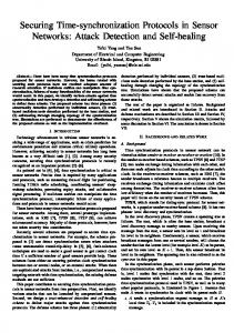
rectness of on-line data timestamping could be observed, since the time headway timestamps were chosen to be the same as the distance timestamps. Fig. 5 shows the timestamping interval increase for one on-line timestamping conversion. It is an extract of about 30 minutes of one experimentation.
Figure 4. The prototype vehicle
Timestamp uncertainty (µs)
400
300
200
converted timestamp intervals 100 original timestamp intervals
post-processing and 19 data in total. There were also dedicated computers for specific indicators, e.g. an eyetracker. There were data with critical times to be recorded, e.g. the time between a stimulus and the corresponding reaction (reaction time). At the end of the experiments, more than 50 parameters were analyzed for the study. Almost 20 drivers were tested. This project led to the development of D-BITE (Driver Behavior Interface Test Equipment) and other works. DBITE also includes a process, with the same characteristics as the one discussed here, for post-processing datasynchronization, thus enabling data recorded during experiments to be post-processed. 5.2.2. Technical description The Microsoft Windows operating system is used, including a multimedia clock allowing a clock granularity which can be inferior to 1 µs, depending on the computer. FireWire is used as synchronous bus network. At present, whereas under Linux RTAI-LXRT, the bus network granularity is better than 5 µs, the granularity is only 130 µs under Windows, but can be improved. The overall framework for these experiments, where there is a substantial volume of data to evaluate, is distributed. Each type of data to be recorded has its own dedicated module. This design makes it possible to equitably distribute the modules between computers. All exchanges of data between modules used on-line timestamping as described in this paper. 5.2.3. Results One of the results is illustrated by time headway timestamp data. The value of the time headway indicator is computed using the following distance (between the host vehicle and the vehicle ahead), given by a radar, and the speed of the host vehicle. As for all modules, one dedicated server handled the distance, and another handled the vehicle speed. A third module with two clients, one for each of the two input data, computed the data timestamps and the time headway. By chance, these operations were done on the same computer, using on-line timestamping as described here, under the Windows operating system. The cor-
0
−100
−200
−300
0
200
400
600
800
1000
1200
1400
1600
1800
Time (s)
Figure 5. Timestamping interval for one online timestamping conversion
In Fig. 5, the original timestamps are the two merged horizontal straight lines in the center, and recomputed timestamping intervals are delimited by the bottom and top lines on the figure. Fig. 5 shows an interval timestamping date increase of about 400 µs per on-line timestamping when the drift estimation is optimum. This result can easily be improved if the bus network clock granularity is improved. Here, no abrupt increases of timestamping uncertainty can be observed, because no bus reset has occurred during this experimentation. It will be noticed that the recomputed interval width is almost constant. This is due to the data request mode: the client asks the server for next data. Data timestamping is therefore carried out on recent data, so the drift component of the recalculation equation almost does not influence. This example shows that the desired timestamp conversion can be used in real experiments.
6. Conclusion This paper has described an on-line timestamping method using interval date timestamping, and presented two examples. This method uses comparisons with a com-
mon clock, the bus network clock, to perform precise on-line timestamp conversions. A first advantage is that no clock is changed on any computer, which allows instantaneously precise on-line timestamping even if the network configuration changes. Furthermore, timestamping uncertainty makes it possible to evaluate its precision. Another advantage is that this on-line timestamping method makes it possible to have more precise timestamping than with methods that use fixed drifts. A final advantage is that few calculations are required to perform the timestamp conversion. It only requires to regularly compute the drift and the conversion is direct: no table is needed to store time equivalences and to find the closest to the timesamp. Several interesting perspectives follow from this work. First, a study of interval timestamping for data fusion is in progress. Obviously, this problem arises when data are not all produced synchronously. It might be interesting to study the consequences of interval date timestamping. Most algorithms do not accommodate interval timestamping. Interval dating takes account of timestamping uncertainty, leading to better data quality estimations. In addition, the desired timestamp conversion can be used in other synchronous bus networks, using for example the Time Triggered Protocol, TTP [8], where a network clock is available. However, whereas the FireWire clock is given by an interface clock, the TTP clock is given by an internal clock synchronization. This means that its drift is not exactly constant, but can vary slightly. In this case it may be supposed that the synchronous bus network clock drift is constant over a given time period which needs to be determined, and then a sliding window can be used to compute the drift.
Acknowledgment The authors would like to thank the members of the Heudiasyc Laboratory who assisted this work. This work is a part of RoadSense project supported by the European Community within the framework of the fifth PCRD.
References [1] D. Anderson. FireWire system architecture (2nd ed.): IEEE 1394a. Addison-Wesley Longman Publishing Co., Inc., 1999. [2] P. Blum, L. Meier, and L. Thiele. Improved interval-based clock synchronization in sensor networks. In Proceedings of the third international symposium on Information processing in sensor networks, pages 349–358. ACM Press, 2004. [3] K. Chaaban, P. Crubillé, and M. Shawky. Scoot-r: a framework for distributed real-time applications. In Proc. of the
[4]
[5]
[6]
[7] [8]
[9]
[10]
[11]
[12]
[13]
[14]
7th int. conf. on princ. of dist. syst., La Martinique, France, December 2003. J. Elson and D. Estrin. Time synchronization for wireless sensor networks. In Proceedings of the 15th International Parallel & Distributed Processing Symposium, page 186. IEEE Computer Society, 2001. J. Elson, L. Girod, and D. Estrin. Fine-grained network time synchronization using reference broadcasts. SIGOPS Oper. Syst. Rev., 36(SI):147–163, 2002. S. Ganeriwal, R. Kumar, and M. B. Srivastava. Timing-sync protocol for sensor networks. In Proceedings of the first international conference on Embedded networked sensor systems, pages 138–149. ACM Press, 2003. L. Jaulin, M. Kieffer, O. Didrit, and Éric Walter. Applied Interval Analysis. Springer-Verlag, June 2001. H. Kopetz. Real-Time Systems: Design Principles for Distributed Embedded Applications, volume 395. Kluwer Academic Publishers, April 1997. K. Marzullo and S. Owicki. Maintaining the time in a distributed system. In Proceedings of the second annual ACM symposium on Principles of distributed computing, pages 295–305. ACM Press, 1983. L. Meier, P. Blum, and L. Thiele. Internal synchronization of drift-constraint clocks in ad-hoc sensor networks. In Proceedings of the 5th ACM international symposium on Mobile ad hoc networking and computing, pages 90–97. ACM Press, 2004. D. L. Mills. Internet time synchronization: The network time protocol. IEEE Transactions on Communications, 39(10):1482–1493, October 1991. S. PalChaudhuri, A. K. Saha, and D. B. Johnson. Adaptive clock synchronization in sensor networks. In Proceedings of the third international symposium on Information processing in sensor networks, pages 340–348. ACM Press, 2004. K. Römer. Time synchronization in ad hoc networks. In Proceedings of the 2nd ACM international symposium on Mobile ad hoc networking & computing, pages 173–182. ACM Press, 2001. U. Schmid and K. Schossmaier. Interval-based clock synchronization. Real-Time Systems, 12(2):173–228, 1997.