On MCMC Sampling in Bayesian MLP Neural Networks Aki Vehtari, Simo Särkkä, and Jouko Lampinen
[email protected],
[email protected],
[email protected]
Laboratory of Computational Engineering Helsinki University of Technology P.O. Box 9400, FIN-02015 HUT, FINLAND Abstract Bayesian MLP neural networks are a flexible tool in complex nonlinear problems. The approach is complicated by need to evaluate integrals over high-dimensional probability distributions. The integrals are generally approximated with Markov Chain Monte Carlo (MCMC) methods. There are several practical issues which arise when implementing MCMC. This article discusses the choice of starting values and the number of chains in Bayesian MLP models. We propose a new method for choosing the starting values based on early stopping and we demonstrate the benefits of using several independent chains.
1 Introduction Multi Layer Perceptron neural networks (MLP) [1] are widely used flexible models suitable in complex nonlinear problems. The main question in MLP models is the estimation of the model parameters. Recently Bayesian methods have become a viable alternative to the older error minimization based (ML or MAP) approaches. Bayesian methods use probability to quantify uncertainty in inferences and the result of Bayesian learning is a probability distribution expressing our beliefs regarding how likely the different predictions are. Predictions are made by integrating over the posterior distribution. See [5] for excellent introduction to Bayesian methods. In case of MLP the posterior distribution is typically very complex. The integrations required by Bayesian approach can be approximated using Markov Chain Monte Carlo (MCMC) methods [10, 3, 23]. An integral Z µ = g(x)p(x)dx (1) can be approximated by MCMC, using a sample of values x(t) drawn from the distribution p(x) µ ˆn ≈
N 1 X g(x(t) ). N t=1
(2)
In the MCMC, samples are generated using a Markov chain that has the desired posterior distribution as its stationary distribution. Due to complex posterior distributions, elaborate MCMC schemes, such as proposed in [15, 16] or [13], are required for efficient sampling in Bayesian MLPs. MCMC is a general strategy, not an algorithm. There are several practical issues which arise when implementing MCMC. For “standard statistical models” many of these issues are discussed in [10, 11] and some of the issues specific for MLPs are discussed in [16] and [13]. Purpose of this paper is to discuss the choice of starting values (Section 2) and the number of chains (Section 3) in Bayesian MLPs. We propose a new method for choosing starting values based on early stopping and we demonstrate the benefits of using several independent chains. We concentrate on Bayesian MLP framework and MCMC schemes described in [16], though most of our discussion is relevant for other MCMC schemes and complex statistical models. We illustrate discussion with demonstration in Section 4.
2 Starting values In theory, if the chain is irreducible, the choice of starting values x(0) will not affect the stationary distribution. In practice, if the chain is slow-mixing, bad starting value may require lengthy burn-in (i.e. we have to run chain longer to get usable samples). Sampling in Bayesian MLP is slow-mixing because of high number of parameters which correlate in posterior distribution. With bad starting values (e.g. values which have very low posterior probability) it might take long time for the chain to traverse to more probable areas. For simple models, with nicely behaving posterior distribution (e.g. low posterior correlations of the parameters), it is usually unnecessary to expend much effort in choosing starting values, though it is recommended that if good starting values are available they are used [6, 9, 10]. Sometimes good starting values can be chosen by using a simpler model (e.g., linear model or fixing hyperparameters), or simpler method (e.g., regularized maximum likelihood). The extra benefit of the approximations is that the final results can be compared to them [5]. Neal [16] has used the hybrid Monte Carlo (HMC) algorithm [2] for the weights and Gibbs sampling [8, 4, 10] for the hyperparameters (the parameters of weight priors and noise model). HMC is an elaborate Metropolis-Hastings Monte Carlo method, which makes efficient use of gradient information to reduce random walk behavior. The gradient indicates in which direction one should go to find states with high probability. Gibbs sampling is perhaps the simplest MCMC method. In a single iteration, Gibbs sampling involves sampling one parameter at time from full conditional distribution given all the other parameters. Gibbs sampling of the hyperparameters given the weights is efficient but HMC sampling of the weights given the hyperparameters is slow-mixing and so good starting values for weights are more important. This is why in following we consider starting values only for the weights of MLP and assume that after we have chosen some values for weights, hyperparameter values are immediately sampled with Gibbs sampling. Usual methods for choosing starting values are Set all parameter values to zero This is reasonable if the parameters have been centered or if the prior belief is that parameter values can be positive or negative with equal probability. This is most commonly used method and this is also used in [16]. Set parameters to prior means This is reasonable if the priors are informative. If the priors are vague the prior mean might be insensible (e.g. if primary reason for the specific prior is its local uniformity in the area where most of the posterior probability is believed to be). In [16] the prior mean for the weights is zero. Sample parameters from prior This is reasonable if the priors are informative. If the priors are vague, sampling from the prior may produce very bad starting values. Weights from vague prior for MLP are very likely to produce very low likelihood (see, e.g., example in [16, pp. 17-19]). Set parameters to MAP estimate This is commonly used in simple statistical models with one or only few not badly skewed modes. MAP estimate can also be used as approximation to which the final result can be compared. In case of MLPs the modes are often badly skewed and the joint MAP for parameters and weights may have almost degenerate solutions in modes. Sample parameters from approximate posterior This is recommended by [7, 6] but it works well only for simple models (or if we have lot of data) when we can easily make reasonable approximations (like Gaussian or tdistribution centered on mode). From these, zero weights are probably the safest starting values for Bayesian MLP. MLP with small weights is almost linear and linear model is usually quite safe initial choice. Very small weights are also usual starting values for gradient based optimization methods in MAP and early stopping solutions. In order to speed up convergence (and so to reduce burn-in time) Neal uses different MCMC algorithm parameters in initial sampling phase(s) and in actual sampling phase [16, 11]. Additionally, in the initial sampling phase hyperparameters are fixed at some value and only the weights are updated. This prevents hyperparameters from taking on strange values in the period before the weights have adopted reasonable values. This is generally a working strategy, but it requires selecting some MCMC parameter values which may differ from the values suitable in the actual sampling. Also it is unclear how long initial sampling phase should be run. In Section 4 we describe a difficult problem where this strategy had problems.
Next we describe a simple, quick and robust method for choosing the starting values based on early stopping. These starting values have high likelihood and no initial sampling phase such as described in [16] is required. 2.1 Starting values with early stopping Early stopping is commonly used regularization method for MLPs [14]. In early stopping weights are initialized to very small values. Part of the training data is used to train the MLP and the other part is used to monitor the validation error. Iterative optimization algorithm is used for minimizing the training error. MLP with small weights is almost linear and non-linearity increases during optimization. Training is stopped when the validation error begins to increase and the weights with minimum validation error are selected. See [20] for discussion about different stopping criteria. The basic early stopping is rather inefficient, as it is very sensitive to the initial conditions of the network and only part of the available data is used to train the model. These limitations can easily be alleviated by using a committee [1] of early stopping MLPs, with different partitioning of the data to training and stopping sets for each network. Early stopping is ad hoc method but it is fast and it has proved to be quite robust method when used as committee of early stopping MLPs. Performance of the (committees of) early stopping MLPs has been compared to Bayesian MLPs, e.g., in [21, 19, 24, 25]. In [22] Rögnvaldsson demonstrated that early stop weights can be successfully used to estimate the weight decay parameter. Weight decay parameter corresponds to Gaussian prior on weights. This supports the idea that early stop weights are reasonable starting values for MCMC sampling in Bayesian MLP. We have used committees of early stopping MLPs as quick preliminary approximations in our case problems [12, 24, 25]. We get quickly some results giving insight to the problem. Then we can use more time to make full Bayesian solution using the early stopping weights as initial guess for MCMC. Finally we can check that our Bayesian solution gives at least as good results as the early stopping approximation. In Section 4 we demonstrate that early stopping starting values worked well in a difficult problem.
3 Number of chains Usually only one chain has been used in MCMC schemes for Bayesian MLPs [16, 21, 13, 19]. In theory one chain is enough in any MCMC simulation, but in practice there is not yet agreement between using one very long chain or several long runs. One-very-long-run school says that one very long run has the best chance of finding new modes and that comparison between chains can never prove convergence. Several-long-runs school says that comparing several seemingly converged chains might reveal differences if the chains have not yet approached stationarity. See detailed discussion in [6, 9]. In simple unimodal problems and problems where one mode is dominant one chain is often adequate. Bayesian MLP usually has multimodal posterior density (see discussion in [13]). In complex multimodal distributions, MCMC algorithms can experience difficulties when high probability areas of the state space are separated by regions of very low probability. Typical schemes have low probability of changing modes and so it may require very long time to visit more than one mode (see also [17, 18] for methods improving sampling of multimodal distributions). If the chain has low probability of visiting several modes, we have found it useful to use several chains. Using dispersed starting values (see Section 2), different chains may end to different modes. Using multiple chains does not give us much information about relative masses of different modes but more elaborate methods are required (see, e.g., [17, 18]). In the next section we describe a difficult problem where we got better results by using more than one chain.
4 Experiment In this section we demonstrate benefits of early stopping starting values and the use of several independent chains in the problem of electrical impedance tomography (EIT). The aim in EIT is to recover the internal structure of an object from surface measurements. Number of electrodes are attached to the surface of the object and current patterns are injected from through the electrodes and the resulting potentials are measured. The inverse problem in EIT, estimating
Hyperparameter value
Hyperarameter value
0
10
−1
10
−2
10
100
200 300 Iteration
400
0
10
−1
10
−2
10
500
(a) Zero weight starting values
100
200 300 Iteration
400
500
(b) Early stop starting values
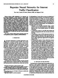
Figure 1: Typical trends for one of the hyperparameters (variance of the first layer weights) during MCMC sampling of Bayesian MLP in electrical impedance tomography (EIT) problem. Note that in practice, after approximate convergence, we used next 100 samples for inference. These chains were run longer for demonstration purposes.
the conductivity distribution from the surface potentials, is known to be severely ill-posed. In [12] we proposed a novel feedforward solution for the reconstruction problem. The approach is based on transformation of both input and output data by principal component projection and application of the MLP in this lower dimensional eigenspace. The reconstruction was based on 20 principal components of the 128 dimensional potential signal and 60 eigenimages with resolution 41 × 41 pixels. Five independent training and test data sets each consisted of 100 simulated bubble formations. MLP networks containing 30 hidden units (2490 weights) were used. Early stop MLPs were made with MATLAB using scaled conjugate gradient optimization and 10-fold split of data. MCMC simulations1 were run with FBM software2 , which implements the methods described in [16]. The length and the number of the chains and the burn-in length were decided using visual inspection of trends and potential scale reduction method [7, 6]. Fig. 1 shows typical trends for one of the hyperparameters (variance of the first layer weights). Chain starting with zero weights is shown at left and chain starting from early stop weights is shown at right. Initial sampling phases used with zero weight starting values helped sometimes, but more often after initial sampling phase the chain was still far away from more reasonable values. Starting values chosen with early stopping were always good. They were near the final samples and no initial sampling phase before actual sampling was needed. Tables 1 and 2 illustrate the benefit of using several chains. Table 1 shows the mean test errors (and standard deviations of means) for different methods calculated with five independent train and test sets. For each five set we run one long chain (2000 iterations) and 10 shorter runs (each 200 iterations) and discarded first 100 iterations from each chain as burn-in. All chains were started with early stop weights. The combined chains method gives lower error than the single long chain method. Note that about same amount of CPU time was used for one long chain and 10 shorter chains. The early stopping MLPs were also used as preliminary estimates and the test errors are included in Table 1. Table 2 shows p-values for pairwise comparisons, obtained from paired t-tests (see [21] or [19] for more details). The combined chains method is significantly better than the other methods (p-value less than 0.01). Fig. 2(a) shows sample distributions of one hyperparameter (variance of the first layer weights) from 10 independent chains. Visual inspection of trends and potential scale reduction method hinted that chains had converged but this figure shows that they are sampling different areas. Fig. 2(b) shows a sample distribution for same hyperparameter from 10 combined chains. 1 The
MCMC sampling specification we used was repeat 20 sample-sigmas heatbath 0.9 hybrid 100:10 0.04 negate
2
Table 1: Performance comparison of various MCMC and reference methods. The task was to approximate the inverse mapping in a tomographic image reconstruction application (EIT, electrical impedance tomography), in order to reconstruct a gas bubble in a liquid flow. The shown errors give the mean percentage of pixels in the test images that were erroneously classified as bubble or background. The values are averaged over 5 independent training and test sets with 100 samples each. See Table 2 for pairwise comparisons Method Early stop MLPs Single early stop MLP Committee of early stop MLPs Bayesian MLPs Single chain (200 iterations) Single long chain (2000 iterations) 10 combined chains (10×200 iterations)
Mean test error % ± std of mean 11.8 ± 0.5 9.5 ± 0.6 9.3 ± 0.5 9.2 ± 0.4 8.6 ± 0.5
Table 2: Pairwise comparisons of various MCMC and reference methods (see Table 1 first). The values in the matrix are p-values, obtained from paired t-tests. The column order of the methods is the same as the row order of the methods. The p-values have been rounded to nearest whole number in percent (so the value 1 indicates a p-value less than 0.01). If the value is larger than 9% it is not considered significant and it is not reported (a dot is shown instead). The p-values are reported in the column of the winning method. Looking row-wise, you see which methods significantly out-performed the method of that row. Method Early stop MLPs Single early stop MLP Committee of early stop MLPs Bayesian MLPs Single chain (200 iterations) Single long chain (2000 iterations) 10 combined chains (10×200 iterations)
·
1 ·
1 ·
· · ·
· · ·
· ·
1 ·
1 1
·
1 1
·
5 Conclusions MCMC methods allow ease use of flexible MLP models in Bayesian framework. We have discussed the choice of the starting values of chains and proposed a new method based on early stopping. Early stopping starting values are quick and easy to generate, they can be used for preliminary estimation and in difficult problems they speed up MCMC sampling. We also showed that the use of several independent MCMC chains may improve the result of Bayesian MLP in a difficult case problem. Using the early stopping starting values and comparing different chains gives us more confidence in the results.
Acknowledgments This study was partly funded by TEKES Grant 40888/97 (Project PROMISE, Applications of Probabilistic Modeling and Search) and Graduate School in Electronics, Telecommunications and Automation.
References [1] Bishop, C. M. (1995). Neural Networks for Pattern Recognition. Oxford University Press. [2] Duane, S., Kennedy, A. D., Pendleton, B. J. & Roweth, D. (1987). Hybrid Monte Carlo. Physics Letters B, 195:pp. 216–222. [3] Gamerman, D. (1997). Markov Chain Monte Carlo: Stochastic simulation for Bayesian inference. Texts in Statistical Science. Chapman & Hall. [4] Gelfand, A. E., Hills, S. E., Racine-Poon, A. & Smith, A. F. M. (1990). Illustartion of Bayesian inference in normal data models using Gibbs sampling. Journal of the American Statistical Association, 85(412):pp. 972–985.
0.25
0.3
0.35 0.4 Hyperparameter value (a) 10 independent chains
0.45
0.25
0.3
0.35 0.4 Hyperparameter value
0.45
0.5
(b) 10 combined chains
Figure 2: Sample distributions of one hyperparameter (variance of the first layer weights) from 10 independent chains (a) and 10 combined chains (b).
[5] Gelman, A., Carlin, J. B., Stern, H. S. & Rubin, D. R. (1995). Bayesian Data Analysis. Texts in Statistical Science. Chapman & Hall. [6] Gelman, A. & Rubin, D. B. (1992). Inference from iterative simulation using multiple sequence (with discussion). Statistical Science, 7(4):pp. 457–472. [7] Gelman, A. & Rubin, D. B. (1992). A single series from the Gibbs sampler provides a false sense of security (with discussion). In J. M. Bernardo, J. O. Berger, A. P. Dawid & A. F. M. Smith, eds., Bayesian Statistics 4, pp. 625–631. Oxford University Press. [8] Geman, S. & Geman, D. (1984). Stochastic relaxation, Gibbs distributions and the Bayesian restoration of images. IEEE Transactions on Pattern Analysis and Machine Intelligence, 6:pp. 721–741. [9] Geyer, C. J. (1992). Practical Markov chain Monte Carlo (with discussion). Statistical Science, 7(4):pp. 473–483. [10] Gilks, W. R., Richardson, S. & Spiegelhalter, D. J., eds. (1996). Markov Chain Monte Carlo in Practice. Chapman & Hall. [11] Kass, R. E., Carlin, B. P., Gelman, A. & Neal, R. M. (1997). Markov Chain Monte Carlo in practice: A roundtable discussion (edited panel discussion). Tech. Rep. 653, Department of Statistics, Carnegie Mellon University. [12] Lampinen, J., Vehtari, A. & Leinonen, K. (1999). Using Bayesian neural network to solve the inverse problem in electrical impedance tomography. In B. K. Ersboll & P. Johansen, eds., Proceedings of 11th Scandinavian Conference on Image Analysis SCIA’99, pp. 87–93. Kangerlussuaq, Greenland. [13] Müller, P. & Rios Insua, D. (1998). Issues in Bayesian analysis of neural network models. Neural Computation, 10(3):pp. 571–592. [14] Morgan, N. & Bourland, H. (1990). Generalization and parameter estimation in feedforward nets: Some experiments. In D. Touretzky, ed., Advances in Neural Information Processing Systems, vol. 2, pp. 630–637. Morgan Kaufman, San Mateo, California. [15] Neal, R. M. (1993). Bayesian learning via stochastic dynamics. In C. L. Giles, S. J. Hanson & J. D. Cowan, eds., Advances in Neural Information Processing Systems, vol. 5, pp. 475–482. Morgan Kaufmann, San Mateo, California. [16] Neal, R. M. (1996). Bayesian Learning for Neural Networks, vol. 118 of Lecture Notes in Statistics. Springer-Verlag. [17] Neal, R. M. (1996). Sampling from multimodal distributions using tempered transitions. Statistics and Computing, 6:pp. 353– 366. [18] Neal, R. M. (1998). Annealed importance sampling. Tech. Rep. 9805, Dept. of Statistics and Dept. of Computer Science, University of Toronto. [19] Neal, R. M. (1998). Assessing relevance determination methods using DELVE. In C. M. Bishop, ed., Neural Networks and Machine Learning, vol. 168 of NATO ASI Series F: Computer and Systems Sciences, pp. 97–129. Springer-Verlag. [20] Prechelt, L. (1998). Early stopping – but when? In G. B. Orr & K.-R. Müller, eds., Neural Networks: Tricks of the Trade, vol. 1524 of Lecture Notes in Computer Science, pp. 55–69. Springer-Verlag. [21] Rasmussen, C. E. (1996). Evaluation of Gaussian Processes and other Methods for Non-Linear Regression. Ph.D. thesis, Department of Computer Science, University of Toronto. [22] Rögnvaldsson, T. S. (1998). A simple trick for estimating the weight decay parameter. In G. B. Orr & K.-R. Müller, eds., Neural Networks: Tricks of the Trade, vol. 1524 of Lecture Notes in Computer Science, pp. 72–92. Springer-Verlag. [23] Robert, C. P. & Casella, G. (1999). Monte Carlo Statistical Methods. Springer Text in Statistics. Springer-Verlag. [24] Vehtari, A. & Lampinen, J. (1999). Bayesian neural networks for image analysis. In B. K. Ersboll & P. Johansen, eds., Proceedings of 11th Scandinavian Conference on Image Analysis SCIA’99, pp. 95–102. Kangerlussuaq, Greenland. [25] Vehtari, A. & Lampinen, J. (1999). Bayesian neural networks for industrial applications. In Proceedings of SMCIA/99 – 1999 IEEE Midnight-Sun Workshop on Soft Computing Methods in Industrial Applications, pp. 63–68. Kuusamo, Finland.