Sampling Conductivity Images via MCMC - CiteSeerX

Sampling Conductivity Images via MCMC Colin Fox and Geoff Nicholls Mathematics Department, Auckland University, Private Bag 92019, Auckland, New Zealand May 1997 Abstract Electrical impedance tomography (EIT) is a technique for imaging the conductivity of material inside an object, using current/voltage measurements at its surface. We demonstrate Bayesian inference from EIT data. A prior probability distribution modeling the unknown conductivity distribution is given. A MCMC algorithm is specified which samples the posterior probability for the conductivity given the prior and the EIT data. In order to compute the likelihood of a conductivity distribution it is necessary to solve a second order linear partial differential equation (PDE). This would appear to make the sampling problem computationally intractable. However by using a Markov chain with Metropolis-Hastings dynamics, and treating the conductivity update as a small perturbation, we are able to avoid solving the PDE for those updates which are rejected by the MCMC sampling process. For real applications the likelihood will need to be sensitive to very small changes in the state, so that the posterior distribution may be sharply peaked as well as multi-modal. The details of the Metropolis-Hastings dynamics are chosen so that ergodic behavior is displayed on useful time scales. We show that the sampling problem is tractable, and illustrate inference from a simple synthetic data set.

1 Introduction Conductivity imaging has been a promising new imaging technique for some time now. The equipment (essentially a current source and a voltmeter) is cheap, portable and non-invasive. Electrodes are attached to the surface of an object, and a small current is applied. The electrical potential is measured (in volts) at points over the surface. This surface potential depends on the unknown conductivity of materials inside the object. In EIT we attempt to reconstruct the conductivity at each point in the object using the known currents and the observed potentials. Consider an open two-dimensional region, with boundary @ . The conductivity  (units ohms?1 ) is an unknown function of position,  (x); x 2 , in the region. Electrodes producing fixed current source distributions J@ = J@ (x) for x 2 @ and J = J (x) for x 2 are applied at the boundary and in the interior of the region. The dimensions of J@ and J are current per unit length and current per unit area respectively. The electrical potential, , is measured along the boundary. When measurements are made at low frequency, Ohm's law (current is proportional to potential gradient), and Kirchoff's law (current is conserved) together imply that within the region the potential satisfies the partial differential equation r
(r) = ?J : (1) Many materials (for example, animal muscle) conduct better along some axes than others. We restrict attention to isotropicly conducting materials, so that  is a scalar. If the region is otherwise insulated, the current crossing into @ is just J@ . Hence if n is the unit outward normal on the boundary @ , the boundary current density is

 @@n = J@ :

(2)

This is just Ohm's Law, and corresponds to a Neumann boundary condition at @ . Note that, since we are assuming conservation of current, there is a consistency condition on the applied currents. Let d (x) be the measure of the element of area at x 2 and let d`(x) be the measure of the element of length at x 2 @ . The applied currents also satisfy Kirchoff's law, Z Z



J (x) d (x) +

J@ (x) d`(x) = 0:

@

(3)

In practice one does not attach current sources in the interior, so J is often zero, and this is the case we treat. The “forward problem” is then to calculate the field  at each x 2 @ given J@ and  . That is, given an applied current distribution J@ satisfying Equation (3), and a conductivity distribution  , find a solution to Equation (1) satisfying the boundary condition Equation (2). The “inverse problem” is, given J@ and  satisfying Equations (1) and (2) for x 2 @ , to find  . We wish to solve the inverse problem. A review of classical methods for regularizing the ill-posed inverse mapping from the data to the conductivity is given in Barber (1989). We propose Bayesian inference based on MCMC sampling of the posterior. Martin and Idier (1997) have given a Bayesian regularization of the inverse problem, extending work by Hua et al (1991). However, these authors use optimization methods as alternatives to sampling. They aim to return just a single state. This cannot, by itself, give any indication of the range of plausible reconstructions. No MCMC has been attempted (including simulated annealing) for an EIT likelihood determined via a PDE. We wish to see to what extent the sampling problem is tractable.

2 The Observation process and Likelihood Suppose K electrodes are attached at the boundary of a region at points xk 2 @ ; k = 1; 2 : : :K . Let E = A pair of electrodes are chosen as anode and cathode and a current of magnitude I0 is applied. A third reference electrode is chosen, and a voltmeter is connected between the reference electrode and each of the other electrodes in turn, not including the anode and cathode, and a potential is measured. Let ean ; ecn and ern denote respectively the label of the anode, cathode, and reference electrode used in each of the n = 1; 2 : : :N electrode arrangements. Let en = fean ; ecn ; ern g. Since there are N = K (K ? 1)=2 distinct anode-cathode choices, we measure N , K ? 3 component vectors, vn ; n = 1; 2 : : :N . We measure one vector vn for each of the current distributions J1 ; : : : JN generated by the n = 1; 2 : : :N distinct current electrode pairs. Note that these measurements are not all independent. We have a total of K (K ? 1)=2  (K ? 3) values in all, while only K (K ? 1)=2 are independent, as we will see. For notational convenience we let vn be a K component vector, so that vn (k ) is the potential measured at the k th electrode in the nth electrode configuration. The redundant components vn (k ) k 2 en are left undefined, since no measurement is made at these electrodes. Let the components of the current due to the n' th electrode pair be Jn = fJ ;n ; J@ ;n g, corresponding to the interior and boundary components of the applied current. We model the electrodes as point sources of magnitude I0 , located at the boundary, so J ;n = 0 and

fx1 ; x2 : : : xK g be the set of electrode positions.

J@ ;n (x) = I0 (x ? xean ) ? I0 (x ? xecn ):

(4)

We assume the electrode positions are measured with negligible uncertainty, and defer discussion of electrode position uncertainty and possible internal electrode structure to later work, in which we treat real data. Let s(x) be the true conductivity at each point x 2 , and let (xjn; s) be the potential at x generated by current distribution Jn in the conductivity s. Refer to Figure 1b for an example. Let (s) denote the N component vector ((xj1; s); (xj2; s) : : : (xjN; s)). We suppose the voltage measurements are made in noise that is additive and Gaussian, mean zero and standard deviation d. Thus if n (k ) is a Gaussian random variable, n (k )  N (0; d2 ), we observe vn (k) = (xk jn; s) + n (k); for each n = 1::N; k = 1::K; k 62 en : (5) The potential at the reference electrode is (xk jn; s) = 0. The solution to the PDE, Equation (1), is determined only up to an additive constant, and by setting (xk jn; s) = 0 we fully determine the solution. Now, given applied currents J and data v , the likelihood of a conductivity distribution  (x) is proportional to exp(L( )), where L( ) is equal to the log-likelihood, L() = ?jv ? ()j=2d2 ; (6) up to a term independent of  , and

jv ? ()j 

N X K X n=1 kk=1 en 62

(vn (k) ? (xk jn; ))2 :

In order to compute (xk jn;  ) we must solve the forward problem for the conductivity  and the current Jn . Thus, to compute the likelihood, we must solve Equations (1) and (2) for (xjn;  ), with J ;n = 0, that is,

with

rx
(rx (xjn; )) = 0

(7)

@(xjn; )=@ nx = J@ ;n ;

(8)

for each n = 1; 2 : : : N . One of the main features of EIT imaging is that information loss occurs in the mapping (s) from the unknown conductivity s to the observable electrode potentials. Even if the potentials are measured perfectly at the electrodes at the boundary, there may still be a great deal of uncertainty in the reconstructed conductivity in the interior.

3 Computing the Likelihood Let current distributions J = (J1 ; J2 : : : JN ) and a conductivity  be given. In order to compute the likelihood of , we need the fields (xjn; ) for x 2 E . That is, we need the field at the electrodes only. Let g (xjy;  ) be the Neumann Green's function for the potential at x 2 given a point-like current source located at y 2 , with a uniform current sink along the boundary. That is, g (xjy;  ) satisfies the PDE

rx
(rx g(xjy; )) = ?(2) (x ? y)

(9)

with

@g(xjy; )=@ nx = 1=j@ j; where j@ j is the length of the boundary. When y 2 @ these relations become

rx
(rx g(xjy; )) = 0

(10)

(11)

and

@g(xjy; )=@ nx = ?(1)(x ? y) + 1=j@ j: (12) Thus when y 2 (respectively, y 2 @ ) the Green's functions are defined by Equations (9) and (10) (respectively

Equations (11) and (12)). In either case, the Green's function is determined up to an additive constant. We fix this “gauge” by referring our Green's functions to a mean zero voltage over the boundary,

Z

g(xjy; ) dl(x) = 0:

@

(13)

It is straightforward to show that the Green's functions we have defined are symmetric, ie, g (yjx;  ) = g (xjy;  ), although this depends delicately on the boundary conditions, Equations (10) and (12), and on the choice of reference potential made in Equation (13). Since the potential fields, (xjn;  ), n = 1; 2 : : :N , satisfy Equations (7) and (8), they are given in terms of the Green's functions by

(xjn; ) = =

Z

Z

g(xjy; )J ;n (y) d (y) + g(xjy; )J@ ;n (y) d`(y) ? 0 (xern jn; )

@

I0 g(xjxean ; ) ? I0 g(xjxecn ; ) ? 0 (xern jn; )

(14) (15)

using Equation (4), where

0 (xern jn; )  I0 g(xern jxean ; ) ? I0 g(xern jxecn ; ): We subtract 0 (xern jn;  ) so that the potential at the reference electrode located at xern is zero. It follows that, in order to compute the N = K (K ? 1)=2 fields (xjn;  ), we must compute K Green's functions, g (xjxk ;  ); k = 1; 2 : : :K , one for each point, xk , at which we attach an anode or cathode. The potential fields are given as linear combinations of this set of “fundamental solutions” by Equation (15). Since the fields we measure depend on just

K Green's functions, no potential measurement can be made at the source electrode, and the Greens functions are symmetric, K (K ? 1)=2 is the number of genuinely independent measurements that can be made on K electrodes. In the examples which follow, we solve for the Green's functions in a square region. We discretize the region in an M -element regular square array (mesh) of pixels labeled m = 1; 2 : : : M . All functions in are approximated by a corresponding function piecewise-constant over pixels. Thus the conductivity  (x), the fields (xjn;  ), and m0 ( ). For the results presented a simple the Green's functions g (xjy;  ) have discrete partners m , m (n;  ) and gm finite difference scheme was implemented in C and called to solve for the Green' s functions. We would do better to concentrate mesh nodes where the solution is a sensitive function of the conductivity and electrode position. We might also choose better basis functions to represent the solution within elements. However the discretization we have given seems to be adequate for simple prototype problems. Notice that the conductivity may be represented via a higher level description (as in Model C below) in which case the pixel conductivity m will be determined by the local conductivity value  (x) in the higher level description. Computing all K Green's functions is a brute force approach and imposes a big computational burden. One of the main tasks in a Bayes/sampling approach to EIT is to find ways to avoid this calculation at each evaluation of a likelihood ratio, and this is what we have done. 4 Modeling the Conductivity We now specify a model for the conductivity distribution in . We assume the true conductivity s is piecewise constant, and takes a finite number C of fixed values C1 ; C2 : : : CC values in . We use a simple clustering model for the conductivity: we represent the conductivity in on the same square mesh we use to solve for ( ), using the same symbol  for the vector of lattice values m , m 2 1; 2 : : :M and the distribution function  (x), x 2 . Let  denote the set of all possible pixel-based conductivity distributions  , so that  2  . We model  on the lattice as an Ising or Potts binary or higher order Markov random field, with distribution

Pr() / exp 

M X m=1

Hm ()

!

where Hm () 

X m m 0

m ;m : 0

(16)

The sum over m0  m is a sum over the four neighbors m0 of m on the square lattice. The function a;b is the indicator function for the event a = b. The posterior for a conductivity distribution  , given observations v is then Pr( jv ) / Pr( ) exp(L( )). We intend to sample the distribution Pr( jv ) and use these samples to answer questions concerning the unknown true conductivity s. The sampling framework which we describe below can be extended to cover more sophisticated priors. Indeed, there would be little point in setting up such a sampler without taking advantage of the flexibility it allows in the modeling stage of the analysis. We proceed now to simply list a few possible improvements which could be made to the prior model. Model A The present model. The types of possible materials in the object are known but not their proportion in area or location. The conductivities of the materials are known exactly, and correspond to the values C1 ; C 2 : : : C C . Model B The types of possible materials (labeled c = 1; 2 : : : C ) are known. The conductivities of these materials vary from one instance to another, but are assumed to have a single uniform value in the sample at hand. The conductivity values Cc , c = 1; 2 : : : C , are supposed to be normally distributed random variables.

Model C We may, in addition, have knowledge about the structure, shape, and arrangement of objects in the regions. For example the region may be known to contain man-made objects, with outlines that are composed of simple geometric structures, such as line-segments and circular arcs. In this case one may use an intermediate or higher level prior, as described, for example, in Grenander and Miller (1993). In this paper we report results for Model A only.

5 Markov Chain Monte Carlo We now define a Markov chain fXt g1 t=0 of random variables Xt taking values in  , and having a t-step distribution Pr(Xt =  jX0 =  (0) ) which tends to the posterior distribution, Pr( jv ), as t tends to infinity. Such a process will generate the samples we require. We use the Metropolis-Hastings method for our Markov chain Monte Carlo as Gibbs sampling is not practicable, on account of the form of the likelihood. In order to get ergodic behavior on useful time scales we found it necessary to include several different types of update in the MCMC. The state is composed of regions of uniform conductivity. Referring ahead, to Figure 1d, we see that much of the uncertainty in the reconstructed state occurs at change points in the conductivity. We therefore focus updates on pixels in regions where the conductivity is non-uniform. This idea can be found in Ripley (1987). There is a second reason why we want to do this. The likelihood is a very sensitive function of pixel conductivity. Changes at conductivity boundaries often make only small changes to the likelihood, and therefore stand a better chance of being accepted. Move 3 below is an example. The simplest way to build multiple moves into a Metropolis-Hastings sampler is to define a separate reversible transition probability for each move type, as in Green (1995). The method is favored over using a single transition probability: in particular, when several moves are allowed to connect the same pair of states, the condition for reversibility is simplified. Let P be the number of moves, and let fPr(p) (Xt+1 = t+1 jXt = t )gP p=1 P be a set of P transition probabilities, reversible with respect to the distribution Pr( jv ). Let p ; p = 1; 2 : : :P , p = 1, be the probability to choose move p. We select a transition probability at random and use it to generate a MCMC update. The overall transition probability is

Pr(Xt+1 = t+1 jXt = t ) =

P X p=1

p Pr (p) (Xt+1 = t+1 jXt = t ):

If at least one of the moves is irreducible on  , then the equilibrium distribution of the chain is Pr( jv ), independent of the choice,  (0) , of starting state. We now list the moves used. The current state is Xt =  , and the move is used to determine a value for Xt+1 . The candidate state proposed in the Metropolis-Hastings scheme is labeled  0 . A pixel n is a near-neighbor of p pixel m if their lattice distance is less than 8. A pixel has twenty four near-neighbors, unless it is on or next to the boundary. An update-edge is a pair of near-neighboring pixels on the lattice. Let N  ( ) be the set of update-edges  () be the set of edges in N  () involving the pixel connecting two pixels of unequal conductivity in  . Let Nm  m. We maintain a list of the update-edges in N (), for the current state  of the Markov chain. We use this to select at random pairs of pixels with unequal conductivities. Let jS j be the number of elements in the set S . Move 1 Flip a pixel. Select a pixel m uniformly at random from 1; 2 : : :M and assign m a new conductivity 0 and chosen uniformly at random from the other C ? 1 possible conductivity values. Call this new value m 0 0 the new conductivity distribution  .  differs from  at just one pixel. The probability to generate the move is q1 ( !  0 ) = 1=M (C ? 1). The acceptance probability is

o n 1 ( ! 0 ) = min 1; e2(Hm( )?Hm ())  eL( )?L() : 0

0

Move 2 Flip a pixel near a conductivity boundary. Pick an update-edge at random from N  ( ). Pick one of  ()j possible ways. the two pixels in that edge at random, pixel m say. Pixel m can be selected in jNm 0 Proceed as in Move 1, generating a candidate state  . The overall probability to generate the move is q2 ( ! 0 ) = jNm ()j=2jN  ()j(C ? 1). The acceptance probability is

  (0 )jjN  ()j  jN m 0 2  ( H (  ) ? H (  )) L (  ) ? L (  ) m m 2 ( !  ) = min 1; e e    0 : 0

0

jNm ()jjN ( )j Swap conductivities at a pair of pixels. Pick an update-edge at random from N  ( ). Suppose it connects

Move 3 pixels

m and n with conductivities m = a and n = b. The candidate state 0 is equal to  except that 0 m = b and n0 = a. The generation probability is q3 ( ! 0 ) = 1=jN  ()j. The acceptance probability is

n o 3 ( ! 0 ) = min 1; e2(Hm( )?Hm ()+Hn ( )?Hn ())  eL( )?L()  jN  ()j = jN  (0 )j : Account has been taken, in the formula for 3 , of the possibility that m and n may be neighbors. 0

0

0

Notice that Move 2 duplicates Move 1, but allows us to focus updates on the interface between regions of differing conductivity as in Ripley (1987). Move 1 is still needed, for irreducibility. Note also that there is no useful simplification of the likelihood ratio exp(L( 0 ) ? L( )), as occurs whenever the posterior random field is Markov. This is because the log-likelihood is not an additive function of  , but depends on the conductivity at each pixel through the non-linear field functions ( ).

6 Markov Chain Monte Carlo with an EIT Likelihood In order to compute the acceptance probabilities, , at an update, we need L( 0 ). This, as was shown in Section 3, involves solving Equations (11) and (12) for the Green's functions g (xjxk ;  0 ) in the candidate conductivity  0 , and computing (xjn;  0 ) and L( 0 ) using Equations (15) and (6). We have described how we solve for the Green's functions. This operation takes too much time to be feasible at each step of the Markov chain. Notice, however, that the two conductivities  and  0 differ only slightly, and that we have already calculated the Green's functions g (xjxk ;  ) in the current conductivity  . Let g (xjxk ; ;  0 )  g (xjxk ;  0 ) ? g (xjxk ;  ) and  (x)  0 (x) ? (x). In terms of these quantities we have, from Equation (11), approximately,

rx
(rx g(xjxk ; ; 0 )) ' rx
(rx g(xjxk ; )) :

(17)

The Green's functions for the operator on the left will satisfy Equations (11) and (12) as before. The term on the right hand side of Equation (17) may be regarded as a current source. If we take Q(xjxk ;  0 )  rx
(rx g(xjxk ; )), we have, as in Equation (14),

g(xjxk ; ; 0 ) '

Z



g(yjx; )Q(yjxk ; ; 0 )d (y)

(18)

We have exploited the symmetry g (xjy;  ) = g (yjx;  ) of our Green's functions in the final step. The important point is that, in order to compute the likelihood, we need the field values at electrodes only. It follows that we need only compute the perturbing field, g (xjxk ; ;  0 ) for x 2 E , ie, for x corresponding to an electrode position. But then the Green's functions on the right hand side of Equation (18) are precisely the Green's functions g (xjxk ;  ) we have available already. Moreover, if the conductivity change  (x) is local, as is usual in MCMC, Q(yjxk ; ;  0 ) is zero over much of . When the integral is reduced to a sum on the lattice variables, this sum is local, involving just a few variables around the point where the change in conductivity is made. The local linearization we have used is good if the term rx
( rx g (xjxk ; ;  0 )) dropped from Equation (17) is small. Similar approximation schemes are possible for Models of type B and C. However, if the conductivity levels Cc ; Cc+1 differ too greatly, for a given PDE mesh, the approximation will be poor. We have only tried this straightforward linearization, however we note that other authors have found that other parameterizations of  give linear approximations with a greater range of accuracy (Martin and Idier 1997) and these may improve our method. The MCMC algorithm is as follows. Given a state Xt =  , given the Green's functions g (xjxk ;  ), for x 2

and xk 2 E , k = 1; 2 : : :K , and given L( ), the log-likelihood of the state, proceed as follows. Step I Select a move p with probability p . Generate  0 by sampling qp (

! 0 ).

Step II Using the local linearization of the present section, estimate L( 0 ). Step III Compute the acceptance probability for the state, p ( Step IV Accept or reject the candidate state  0 :

!  0 ).

IV.i If  0 is rejected, set Xt+1 =  . Since there is no change to the state, the Green's functions and loglikelihood are unchanged, available for the next iteration. IV.ii If  0 is accepted, set Xt+1 =  0 . We must now solve Equations (11) and (12) to compute g (xjxk ;  0 ), for k = 1; 2 : : :K , and update the log-likelihood to L( 0 ).

To summarize, given the Green's functions for current sources in a conductivity  , we may estimate the likelihood of a candidate conductivity  0 generated in the Metropolis-Hastings procedure, without solving the PDE again. Metropolis-Hastings updates which lead to rejection are local operations, involving the conductivity values at just a few pixels neighboring the point at which a change is made. However, if  0 is accepted, we must solve the PDE, as we now wish to perturb about the fields of the conductivity  0 .

7 Experiments The algorithm described in Section 6 was implemented in C. The MCMC software was tested (to an accuracy of about 1 part in 1000) by taking an independent sequence of MCMC runs, and varying between runs those parameters of the Markov process which leave the equilibrium distribution undisturbed. In particular we can use different sets of  -values in different runs. In this way we vary the proportions of the moves used. We can then check, by comparing the values of statistics estimated from the output, that all the moves preserve the same stationary distribution. We can also vary the number of update-edges at each p pixel. We p experimented with four, eight and twenty four update-edges, corresponding to near-neighbors out to 1, 2 and 8 lattice units. In the following example we start with the known conductivity distribution, s(x), shown in Figure 1a, along with the locations of the sixteen electrodes. The conductivity model and the finite difference PDE solver use the same 25  25 conductivity lattice. We condition on the value of the conductivity at the boundary itself, so Xt (x) = s(x) for x 2 @ and all t. The two grey-levels correspond to two conductivities (C = 2) of C1 = 1 and

a

b

1

c

0.5

0

−0.5

−1

−1.5 25

20

15

10

5

30 0

20

10

0

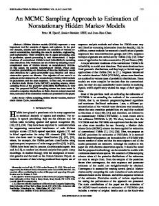
Figure 1: Recovering conductivity information for a synthetic data set, computed from (a). The dots around the boundary in (a) are the electrode locations. The graph in (b) is the potential field (xjn; s) for the conductivity in (a), for one of the n = 1; 2 : : : 120 fields. The state in (c) was obtained after about 10 minutes time on the reference machine, (see below). The mean conductivity from a long run is shown in (d).

C2 = 2 conductivity units. A binary Markov random field is a reasonable prior for distributions of this kind, and we choose a prior parameter value  = 1. The potential fields (xjn; s); n = 1; 2 : : :N are computed for x 2 . The computed potential for one such electrode pair is shown in Figure 1b. Artificial data v is generated by adding Gaussian noise to the potential observed at each electrode, as in Equation (5). We choose to test observations with standard deviation d = 0:005, a signal to noise ratio of around 1500 : 1, taking account of the (K ? 3)-fold over-measurement. Hua et al (1991) find such SNR's physically achievable. We run MCMC using moves 1, 2 and 3 in the proportions 1:9:81, with the chain initialized to a random conductivity at each pixel. The state shown in Figure 1c was reached after 100 sweeps (1 sweep = M Markov chain steps), which took less than about 10 minutes on readily available hardware ( a Pentium Pro 200 costing about three thousand pounds in 1997 ). The posterior mean conductivity at each pixel from a run of 50,000 sweeps is shown in Figure 1d. We might just as easily plot the variance at each pixel, or any other summarizing statistic of interest. Has the MCMC converged ? The log-likelihood is plotted against sweeps in Figure 2. Standard tests shown no sign of slow mode-hopping, and give an integrated auto-covariance time (for the number of pixels at a given conductivity level) of 27(5) sweeps. We are getting an effective independent sample each 90 seconds. Other statistics were considered and have similar behavior. The acceptance rate for updates is low, only 0.6%. The high computational cost of an acceptance is balanced against the more common but faster rejections. The approximation Equation (18) is therefore most important, as the PDE need only be solved in the event that an update is accepted. The approximation leads to an error rate of 14%: that is, 14% of the acceptances would not occur if the likelihood was calculated without approximation.

d

−800 −810

L(θ) −820 −830

0

10000

20000

30000

40000

50000

MCMC updates (sweeps)

Figure 2: The sample log-likelihood (up to a constant independent of  ) plotted against the update number.

8 Conclusions We found that a Bayesian approach to inverting EIT data, with analysis based on posterior samples obtained via MCMC simulation, was feasible, for simple two-level synthetic problems. We have experimented with conductivity distributions in which there are three or more conductivity levels, using a multi-level Markov random field or Potts model, and again, found it possible to treat simple structures with the methods described here. However, several problems remain. At noise levels low enough to define more delicate structures, the MCMC sticks in unrepresentative states. It seems to be possible, in many cases, to recover ergodicity by adding new types of moves to the MCMC. Viewing the state of the MCMC, Xt , evolving as t increases can be helpful. Pixels near the boundary cause particular difficulty at the convergence stage. Indeed, a Bayesian/sampling approach may be inappropriate for reconstruction near the boundary, where there is little uncertainty in the conductivity. However, we expect that higher level models, of the kind described in Section 4, Model C, and explicitly in this workshop, will resolve the problem in a more general way, for at least some electrode arrangements and conductivity distributions. Higher level models remove or change the character of the ambiguity in the reconstruction. This ambiguity corresponds to multi-modality in the posterior, which is the immediate difficulty. It is clearly necessary to test the approach on real data. With synthetic data, the effects of discretization are canceled, since the forward and inverse problems are solved under the same approximation. Real data introduces a number of new problems, such as modeling electrode structure, and allowing for uncertainty in electrode position, which will greatly increase the computational burden of computing a likelihood ratio. However there remain a number of ways in which our computational procedure may be accelerated, and so we consider it at least possible that the sampling problem will continue to be tractable.

References Barber, D.C. (1989). A review of image reconstruction techniques for electrical impedance tomography Med. Phys., 16:162–169. Green, P. (1995). Reversible jump MCMC and Bayesian model determination. Biometrika, 82:711–732. Grenander, U. and Miller, M. (1993). Representation of knowledge in complex systems (with discussion). Journal of the Royal Statistical Society B, 56:549–604. Hua, P., Woo, E., Webster, J. and Tompkins, W. (1991). Iterative reconstruction methods using regularization and optimal current patterns in electrical impedance tomography. IEEE Trans. Med. Imag., 621–628. Martin, T. and Idier, J. (1997). A Bayesian non-linear approach for electrical impedance tomography Technical Report, Lab. des Signaux at Systems, CNRS, Plateau de Moulon, 91192 Gif-sur-Yvette Cedex, France. Ripley, B. D. (1987). Stochastic Simulation. Cambridge University Press, Cambridge.